CHAPTER 18
Array Functions and Formulae
INTRODUCTION
This chapter presents a general discussion of array functions and formulae. It is worth treating these before presenting many other Excel functions: not only are array functions present in several Excel function categories, but also essentially any Excel function can be used as part of an array formula. The chapter covers the core principles, which are used at various places elsewhere in the text.
Functions and Formulae: Definitions
The essential feature of array functions and formulae is that “behind the scenes” they perform calculations that would otherwise be required to be conducted in several ranges or multi-cell tables. The output (return statement) of an array function generally extends over a range of multiple contiguous cells; however, some return values only to a single cell.
The distinction between functions and formulae is:
- Array functions are in-built Excel functions which inherently require the use of a contiguous array in their calculations or output form. They are a type of function, not a separate function category. Examples include TRANSPOSE (Lookup and Reference category), MMULT, MINVERSE (Math&Trig category) and FREQUENCY and LINEST (Statistical category). Some user-defined functions that are created using VBA macros may also be written to be array functions.
- Array formulae use standard Excel functions or operations (such as SUM, MIN or IF), but are written so that intermediate calculation steps are performed inherently “behind the scenes”, rather than explicitly calculated in multi-cell Excel ranges.
Implementation
Array functions or formulae must be entered by placing the cursor within the Formula Bar and pressing Ctrl+Shift+ENTER. The cell range over which they are to be entered can be selected immediately before the formula is built, or after it has been built within the first cell of the range (in which case Ctrl+Shift+ENTER needs to be used again).
Advantages and Disadvantages
In some specific contexts, array functions are almost unavoidable, as the alternatives are much less efficient (the examples provided later in this chapter and in the subsequent text should make this clear). On the other hand, the use of array formulae is generally a choice. Possible benefits include:
- To create more transparent models, in which the explicitly visible part focuses on displaying inputs, key outputs and summary calculations, whereas tables of intermediate calculations (whose individual values are of no specific interest) are conducted behind the scenes.
- To create formulae which are more flexible if there are changes to the size of the data range or the time axis.
- To avoid having to implement some types of calculation as VBA user-defined functions.
There are several disadvantages in using array functions and formulae:
- Entering the formula incorrectly (e.g. by using just ENTER instead of Ctrl+Shift+ENTER) could result in an incorrect value (such as zero) appearing in the cell; the main danger is that such values may not obviously be wrong, and so may be overlooked (in contrast to the cases where a #VALUE message appears). Thus, inadvertent errors may arise.
- Many users are not familiar with them, which may result in the model being harder for others to understand or interpret (or where the user may accidentally edit a formula and return ENTER).
- In some cases, their presence can slow down the calculation of a workbook.
PRACTICAL APPLICATIONS: ARRAY FUNCTIONS
Example: Capex and Depreciation Schedules Using TRANSPOSE
The TRANSPOSE function can be used to turn data or calculations that are in a row into a column, and vice versa. Such a transposition can be performed explicitly within an Excel range, or embedded within a formula.
The file Ch18.1.SUMPRODUCT.TRANSPOSE.1.xlsx shows an example of each approach within the context of “triangle-type” calculations for depreciation expenses (as presented in Chapter 17).
On the “Range” worksheet, the TRANSPOSE function is used to explicitly create a range which contains the capex data in a column (cells C9:C14), so that this data set can be multiplied with the column data of depreciation percentages using the SUMPRODUCT function (see Figure 18.1).
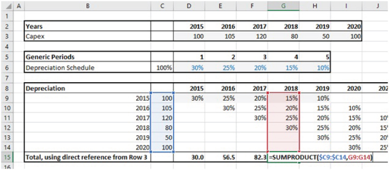
FIGURE 18.1 Using TRANSPOSE to Transpose a Data Range
On the “Formula” worksheet, the transposed capex data is not entered explicitly in Excel; rather it is implicitly embedded as an array, by using TRANSPOSE within the SUMPRODUCT formula (see Figure 18.2).

FIGURE 18.2 Using TRANSPOSE Embedded Within a Formula
Example: Cost Allocation Using SUMPRODUCT with TRANSPOSE
The file Ch18.2.SUMPRODUCT.TRANSPOSE.2.xlsx shows an application to the allocation of the projected costs of a set of central overhead departments to business units, based on an allocation matrix; a screen-clip of the file is shown in Figure 18.3. Once again, the TRANSPOSE function is used within SUMPRODUCT to ensure that the data sets being multiplied are implicitly both row (or both column) data; the alternative would be to explicitly transpose all the data in one of the two input data ranges.

FIGURE 18.3 Use of TRANSPOSE with SUMPRODUCT in Cost Allocation
Example: Cost Allocation Using Matrix Multiplication Using MMULT
Excel has several array functions that relate to mathematically oriented approaches. In fact, the cost allocation example shown in Figure 18.3 can also be considered as a matrix multiplication in which a single row vector and a single column vector are multiplied together using MMULT. Note that when doing so, per standard mathematical convention, the row vector must be the first of the two function-argument entries, and no transposition of the data is required.
The file Ch18.3.MMULT.1.xlsx shows an implementation of this in the cost allocation example used above; a screen-clip is shown in Figure 18.4.

FIGURE 18.4 Use of MMULT in Cost Allocation
Example: Activity-based Costing and Resource Forecasting Using Multiple Driving Factors
When building a model to forecast the resources required to be able to achieve and deliver a desired revenue profile, one may have some resources whose activities are determined by several underlying factors. One may have a few examples, or be able to make estimates of possible scenarios in terms of the resource level required for different levels of activity drivers; from these, one can determine the scaling coefficients (under the assumption of a linear scaling from activity levels to resource requirements).
For example, if a resource (staff) level of 30 is observed to serve 25 customers spread over 150 sites, whereas 35 staff are needed to serve 20 customers over 200 sites, one may write this in terms of activity coefficients:
where R denotes the resource level, S the number of sites and C the number of customers. If the equations corresponding to the two specific cases are written in full, then matrix algebra can be used to solve for the coefficients A0 and A1.
The file Ch18.4.CostDriverForecasting.xlsx contains an implementation of this (see Figure 18.5). Note that if the coefficients A0 and A1 are considered as the components of a column vector, they are the solution to the equation:

FIGURE 18.5 Using Array Functions for Matrix Calculations to Calculate Cost Driver Coefficients
where R is the set of resources used (cells C5:D5), D is the detailed data of sites and customers (cells C3:D4), and T represents the transpose operation. Therefore, A can be found by inverting the transpose of D and multiplying by the resource vector:
Rows 7 through Row 18 shows the individual steps of this operation (which could be combined into a single column range if desired, rather than broken out as individual steps). Once the components are determined, they can be applied to a new case (or cases) that would arise in a forecast model (in which the number of customers and sites is forecast, and this part of the model also determines the resource requirements), as shown in cells C21 to C23. The array functions used are TRANSPOSE, MINVERSE and MMULT.
Example: Summing Powers of Integers from 1 Onwards
The MINVERSE array function finds the inverse of a square matrix (mathematically inclined readers may also wish to use MDETERM to check that its determinant is non-zero, and hence that an inverse can be found). Although the function has several uses in more advanced financial applications (such as optimisation of portfolios of financial assets, and in determining risk-neutral state prices, amongst others), at this point in the text we will use it to find the solution to a general numerical problem.
For example, it is well known that the sum of the integers from 1 to N is given by:
or:
As is commonly known, this formula can be derived simply by writing out the set of integers twice, once in the natural order and once in reverse order: this creates N pairs of integers, each of which sums to N+1.
In order to more clearly relate this to the discussion below, we note that:
In a next step, one may wish to find an expression for the sum of a power of each of the integers from 1 to any number N (e.g. sum of the squares of each integer, or sum of the cubes of each integer). In order words, for a chosen power, p, we aim to find an expression for:
Since there are N terms and the power is p, we can hypothesise that the desired expression is of the form:
For example, in the case that ![]() , we may hypothesise that
, we may hypothesise that
with the coefficients Ci still to be determined (for i=0 to 3).
If the sum of the squares is evaluated for each integer (i) from 0 to 3, we obtain:
Thus:
One can immediately see that ![]() (and that this would be the case for any power of p); this coefficient is therefore left out of the future discussion.
(and that this would be the case for any power of p); this coefficient is therefore left out of the future discussion.
One way to find the value of the remaining coefficients is to solve by repeated substitution (first a forward pass, and then a backward pass): for the forward pass, first, C1 is eliminated by using the second equation to write:
The third equation then becomes:
This can be rearranged to express C2 in terms of C3:

The fourth equation can then be written entirely in terms of C3, by substituting the terms involving C1 for C2, and then similarly C2 for C3, to arrive at an equation that involves only C3 i.e:

This gives:
The backward pass then calculates C2 from C3 (to give ![]() ), and then C1 from C3 and C2 (to give
), and then C1 from C3 and C2 (to give ![]() ), so that:
), so that:
On the other hand, instead of explicitly solving the equations in this way, one could use matrix algebra to express the last three equations (since the first equation has solution ![]() ) as:
) as:

Therefore, the vector of Ci can be found by matrix inversion:

This can be readily calculated in Excel using the MINVERSE function.
The file Ch18.5.MINV.SumofPowers.xlsx shows these calculations, as well as the coefficients that result for the first, second, third, fourth and fifth powers. Note that the results are formatted using Excel's Fraction formatting option; Figure 18.6 shows a screen-clip.

FIGURE 18.6 Calculation of Sums of the Powers of Integers Using MINVERSE
From the results, we see:
Of course, the equations for higher powers may also readily be derived by extending the procedure.
PRACTICAL APPLICATIONS: ARRAY FORMULAE
Example: Finding First Positive Item in a List
In Chapter 17, we noted that the “MAXIF” or “MAXIFS” functions were introduced into Excel in 2016. Prior to this (and hence in some models built before this time), the functionality could have been achieved by combining the MAX (or MIN) and IF functions in an array formula.
The file Ch18.6.MAXIF.MINIF.FirstCashFlow.xlsx shows an example, used in the context of finding the date of the first negative and first positive values in a time series (note that other approaches, such as lookup functions, can also be used; see Chapter 25); Figure 18.7 shows a screen-clip.

FIGURE 18.7 Combining the MIN and IF in an Array Formula to Find Dates of First Cash Flows
The array formulae embed an IF statement within a MIN function to find the minimum (in a set of numeric dates) for which a condition is met (either that the cash flow is positive or that it is negative). For example, the formula in Cell C7 is:
Note the syntax of the IF function within the formulae: there is no explicit statement as to the treatment of cases where the condition (such as E7:Bl7<0) has not been met; the formulae explicitly refer to the date range only for cases in which the condition is met. One may try to make such cases more explicit, for example by using a formula such as:
However, the result would be a minimum of zero (in this case), as whenever the condition is not met, the result of the IF statement will evaluate to zero, which would then be multiplied by the corresponding numerical (positive) date, to give a set of data which is either positive or zero (and thus has a minimum of zero). The fact that the treatment of cases in which the condition is not met is not shown explicitly does reduce transparency, since one must know (or may have to pause to consider or test) how the array formula is treating such cases. This may be a reason to be cautious of using such approaches if other alternatives are available.
The file also shows the equivalent calculations using the MAXIFS and MINIFS functions (which are not shown in the screen-clip, but can be referred to by the interested reader).
Example: Find a Conditional Maximum
One may generalise the method in the prior example to find conditional maxima or minima, subject to the application of multiple criteria.
The file Ch18.7.MAXIF.MAXIFS.DataSet.xlsx shows an example in which one wishes to find the maximum of the “Amount £” field, both for a customer or country, and for a customer–country combination. Figure 18.8 shows a screen-clip, with the file containing formulae IF statements such as:

FIGURE 18.8 Application of Multiple Criteria Using Array Formulae to Calculate Conditional Maxima and Minima
Note that, as shown in cells G10 and G11:
- Once again, attempting to make more explicit the case where the criteria are not met (cell G10) is likely to result in incorrect calculations (the minimum appears to be zero, due to the conditional not being met, rather than the true minimum, which is a -11862 in Cell E16).
- Using a single (non-embedded) IF function would also not be correct.
Example: Find a Conditional Maximum Using AGGREGATE as an Array Formula
The above examples have shown that although one can use array formulae to calculate conditional maxima and minima, there are some disadvantages, including that the treatment of cases where the condition is not met is not very explicit, and that the application of multiple criteria will often require embedded IF statements.
The AGGREGATE function (Excel 2013 onwards) could be used as an alternative. One advantage is that the nature of the calculation could rapidly be changed or copied (i.e. instead of a maximum or minimum, one could switch to the average) using the wide set of function types possible (as shown in Chapter 17, Figure 17.19).
To use the function in the context of a conditional query, one creates a calculation which results in an error when the condition is not met, and uses the function in the form in which it ignore errors (Option 6).
As we are using an array formula, the array form (not the reference form) of the AGGREGATE function should be used; that is, for the maximum, we use the LARGE function (not MAX) and for the minimum we use SMALL (not MIN). In both cases, the (non-optional) k-parameter is set to 1.
The file Ch18.8.MAXIFS.AGGREGATE.xlsx shows an example (see Figure 18.9).

FIGURE 18.9 Example of Using an Array Formula with AGGREGATE to Calculate the Conditional Maximum of a Data Set
Columns J through M of the same file show how the calculations can also be performed directly using the non-array form of the AGGREGATE function, so long as the calculations that are implicit (behind the scenes) for the array formula are conducted explicitly in Excel (see Figure 18.10). Thus, the array formula can save a lot of space and may be easier to modify in some cases (e.g. as the size of the data set is altered). Note that the equivalent calculations could not be performed with the MIN or MAX functions, as these are not allowed to have errors in their data sets.

FIGURE 18.10 Using the Non-array Form of the AGGREGATE Function Based on Explicit Individual Calculations