
CHAPTER 32
Manipulation and Analysis of Data Sets with VBA
INTRODUCTION
This chapter focuses on the use of VBA in the manipulation and analysis of data sets. In fact, almost all of the necessary techniques used here have already been mentioned earlier; to some extent this chapter represents the integration and consolidation of these within the specific context of data analysis.
PRACTICAL APPLICATIONS
The examples in this section include:
- Working out the size of a given data range.
- Defining the data set at run time, based on user input.
- Defining the data set at run time by automatically detecting its position.
- Reversing the rows and/or columns of a data set (either into a new range, or in place).
- Automation of general Excel functionalities.
- Automation of processes to clean data sets, such as deleting rows containing blanks.
- Automation of the use of filters to clean, delete or extract specific items.
- Automation of Database function queries.
- Consolidation of several data sets that reside in different worksheets or workbooks.
Example: Working Out the Size of a Range
One of the most compelling reasons to use VBA to manipulate or analyse data sets (rather than build the corresponding operations using Excel functions and functionality) is that VBA can detect the size of a data set, and conduct its operations accordingly. By contrast, if the size of a data set changes, then Excel functions that refer to this data would generally need to be adapted as well as copied to additional cells (unless dynamic ranges or Excel Tables are used, as discussed earlier in the text). As mentioned in Chapter 29, the use of the CurrentRegion property of a cell or range is one very important tool in this respect.
The file Ch32.1.Current.Region.xlsm contains an example (see Figure 32.1). In the file, Cell B2 has been given the Excel named range DataSetStart, and it is assumed that any new rows or columns that are added to the data set will be contiguous with existing data. The worksheet containing the data has been given the VBA code name DataSheet, so that in this example, we assume that there is only one such worksheet.
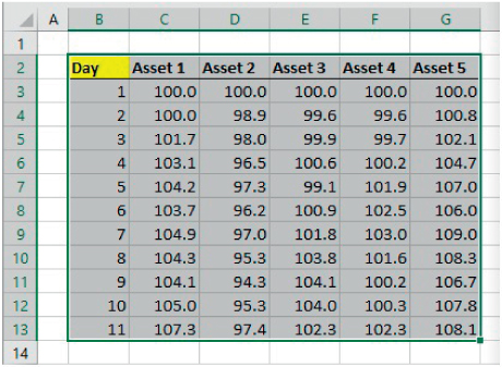
FIGURE 32.1 Using CurrentRegion to Detect the Size of a Range
The screen-clip shows the effect of running the following code, which selects the entire data range.
Sub MRSelectDataWith DataSheetRange("DataSetStart").CurrentRegion.SelectEnd WithEnd Sub
Note that in practice (as mentioned earlier), it is usually best to conduct directly the operation that is desired without selecting ranges. Thus, code such as the following could be used to directly define the data set (as an object variable called DataSet):
Sub MRDefineData1()Set DataSet = Range("DataSetStart").CurrentRegionEnd Sub
Generally, the number of rows and columns in the data set would wish to be known, which could be established by code such as:
Set DataSet = Range("DataSetStart").CurrentRegionNRows = DataSet.Rows.CountNCols = DataSet.Columns.Count
Example: Defining the Data Set at Run Time Based on User Input
In many cases, one may not wish to have to pre-define an Excel cell or named range within a data set, but instead to have the user identify the starting (or any other) cell of the data, assuming a contiguous data set. As mentioned in Chapter 29, an Application.InputBox can be used take a cell reference from the user at run time, for example:
Set dInputCell = Application.InputBox("Select Any Cell within Data Range", Type:=8)One can then define the data range as being (for example) the current region associated with that particular input cell:
Set DataSet = dInputCell.CurrentRegionThe file Ch32.2.InputBoxCellRef.xlsm contains an example of this, and Figure 32.2 shows the part of the process step where a user may identify any cell within the data range as an input cell, from which the full data range is established:
Sub MRCountDataRowsCols()Set dInputCell = Application.InputBox("Select Any Cell within Data Range", Type:=8)Set DataSet = dInputCell.CurrentRegionNRows = DataSet.Rows.CountNCols = DataSet.Columns.CountEnd Sub
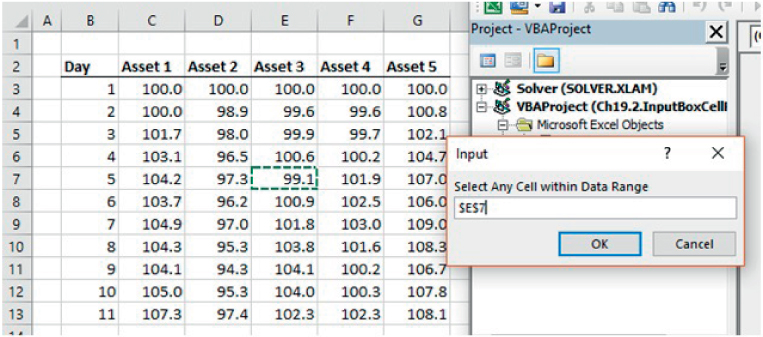
FIGURE 32.2 Taking User Input About the Location of a Cell or Data Point
Example: Working Out the Position of a Data Set Automatically
Of course, asking the user to be involved in defining the data set may not be desirable or may limit one's ability to automate the identification of multiple data sets (for example, that are each contained in a separate worksheet). Thus, one may wish to automate the process of inspecting a worksheet to detect the data range. Important tools in this respect are those that detect the used range and the last cell that is used in a worksheet.
The file Ch32.3.DataSizeGeneral.xlsm contains the code described below, and an example data set on which it can be tested. The used range on a worksheet can be determined with code such as:
With DataSheetSet dRange = .UsedRangeEnd With
In applications where there are multiple worksheets, some of which may need to be deleted or added during code execution, most frequently the worksheet names would be Excel worksheet names, rather than code names. (For example, the worksheets may have been inserted automatically though the running of other procedures, and not have code names attached to them, as described in Chapter 31.) In this case, the code would be of the form:
With Worksheets("Results1")Set dRange = .UsedRangeEnd With
The first cell of the used range could be set using:
Set dstart = .UsedRange.Cells(1, 1)Similarly, the code syntax .UsedRange.Address can be used to find the address of the data set and report it using a message box when the code is run (see Figure 32.3).
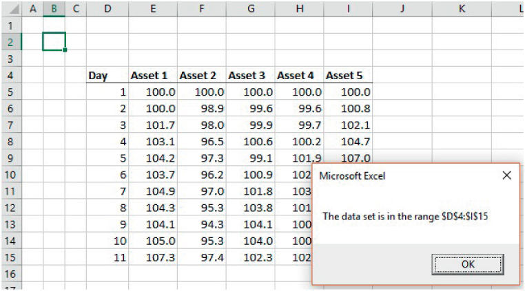
FIGURE 32.3 Finding the Full Range of any Single Contiguous Data Set
Once the full data set is defined, its row and columns can be counted, so that the last cell of the data set would be given by:
NRows = DataSet.Rows.CountNCols = DataSet.Columns.CountSet LastCell = DataStart.Cells(NRows, NCols)
Alternatively, the last cell could be identified using the code discussed in Chapter 29, arising from recording a macro as Excel's GoTo/Special operation is conducted:
With Worksheets("Data").Range("A1")Set lcell = .SpecialCells(xlCellTypeLastCell)End With
Example: Reversing Rows (or Columns) of Data I: Placement in a New Range
The techniques to detect the location and size of data sets are generally a precursor to subsequent operations. A simple example could be the need to reverse the order of all the rows (and/or columns), such as for a data set of time series.
The file Ch32.4.ReverseAllRowsExceptHeaders.xlsm contains the code which uses the methods above to detect and define a data set of contiguous data, and then reverses all its rows, except for the header. The new data is placed one column to the right of the original data, and the headers are copied across (Figure 32.4 shows the result of running the code):
Sub ReverseDataRows()With Worksheets("Data")Set DataStart = .UsedRange.Cells(1, 1)Set DataSet = DataStart.CurrentRegionNRows = DataSet.Rows.CountNCols = DataSet.Columns.CountWith DataStart.Cells(1, 1)For j = 1 To NColsFor i = 2 To NRows.Offset(NRows - i + 1, NCols + j).Value = .Offset(i - 1, j - 1).ValueNext i'copy the label across.Offset(0, NCols + j).Value = .Offset(0, j - 1).ValueNext jEnd WithEnd WithEnd Sub
FIGURE 32.4 Reversing Data and Placing the Results Next to the Original Data
(Note that the code has been written to leave a column gap between the original and the reversed data. This ensures that the CurrentRegion of .UsedRange.Cells(1,1) refers only to the original data set.)
In more general cases, one may wish also to reverse the column order of the data. This is possible by a straightforward adaptation, in which the indexation number on the left-hand side of each assignment statement (i.e. those for the value and for the labels) is modified, by replacing NCols + j with 2 * NCols + 1 – j. This results in the columns being worked in reverse order; this code is also included in the example file.
Example: Reversing Rows (or Columns) of Data II: In Place
One can also manipulate data “in-place”, rather than writing the results to a separate range. A simple way to do this is to read the original data into a VBA array as an intermediate step, and then read the results from the array back into Excel (thereby overwriting the original data range).
The file Ch32.5.ReverseInPlaceArray.xlsm contains an example, using the following code:
Sub ReverseDataRowsArray()Dim aData()With Worksheets("Data")Set DataStart = .UsedRange.Cells(1, 1)Set DataSet = DataStart.CurrentRegion'Set dpoint = Application.InputBox(prompt:="Select a cell in the data range", Type:=8)'Set DataSet = dpoint.CurrentRegionNRows = DataSet.Rows.CountNcols = DataSet.Columns.CountReDim aData(1 To NRows, 1 To Ncols)With DataStart.Cells(1, 1)' //// READ INTO THE ARRAYFor j = 1 To NcolsFor i = 2 To NRowsaData(i, j) = .Offset(i - 1, j - 1).ValueNext iNext j' //// WRITE FROM THE ARRAYFor j = 1 To NcolsFor i = 2 To NRows.Offset(i - 1, j - 1).Value = aData(NRows + 2 - i, j)Next iNext jEnd WithEnd WithEnd Sub
Note that the step in the earlier code in which the header is copied is no longer necessary in this example, as the data remains in place and the columns are not reversed.
Example: Automation of Other Data-related Excel Procedures
One can automate many standard Excel operations by adapting the macros that result from recording operations, often using some of the range-identification techniques above when doing so. These could include:
- Clearing ranges.
- Removing duplicates.
- Applying Find/Replace.
- GoTo/Special Cells (e.g. selection of blanks, dependents, precedents etc.).
- Sorting.
- Refreshing PivotTables.
- Inserting SUBTOTAL functions using the Wizard.
- Inserting a Table of Contents with Hyperlinks to each worksheet.
- Using Filters and Advanced Filters.
Examples of some of these have been provided earlier in the text. Here, and later in this chapter, we discuss a few more.
The file Ch32.6.ClearContentsNotHeaders.xlsm shows an example (containing the following code) that uses the ClearContents method to clear an entire data range, except for the first row (which is assumed to contain heads that wish to be retained):
Sub DeleteDataExceptHeaders()With Worksheets("Data")Set DataStart = .UsedRange.Cells(1, 1)Set DataSet = DataStart.CurrentRegionNRows = DataSet.Rows.CountNCols = DataSet.Columns.CountWith DataStartSet RangeToClear = Range(.Offset(1, 0), .Offset(NRows - 1, NCols - 1))RangeToClear.ClearContentsEnd WithEnd WithEnd Sub
(In practice, some additional code lines or error-handling procedures may be added to deal with the case that no data is present, i.e. only headers for example, such as would be the case if the code were run twice in succession.)
The file Ch32.7.FindSpecialCells.xslm contains another similar example; this shades in yellow all precedents of a selected cell. To achieve this, two macros were recorded, combined and adapted: the first uses GoTo/Special to find the precedents of a selected cell or range, and the second shades a selected range with the colour yellow. The code also has an error-handling procedure which overrides the warning message that would appear if the cell or range has no precedents (and a button has been set up in the file, so that the macro could be used repeatedly and easily in a larger model).
Sub ColorAllPrecedentsYellow()On Error GoTo myMessageSelection.Precedents.SelectWith Selection.Interior.Color = 65535End WithExit SubmyMessage: MsgBox "no precedents found"End Sub
Example: Deleting Rows Containing Blank Cells
One can select all blank cells within an already selected range by using the GoTo/Special (F5 short-cut) functionality in Excel. When this is recorded as a macro, one has syntax of the form:
Selection.SpecialCells(xlCellTypeBlanks).SelectThis is easily adapted to create code which will delete all rows in a selection that contains blank cells (and with the addition of an error-handler to avoid an error message if there are no blank cells in the selection):
Sub DeleteRowsinSelection_IfAnyCellBlank()On Error Resume Next 'for case that no blank cells are foundSet MyArea = Selection.SpecialCells(xlCellTypeBlanks)Set rngToDelete = MyArea.EntireRowrngToDelete.DeleteEnd Sub
The file Ch32.8.DaysLateAnalysis.DeleteRows1.xlsm contains an example. Figure 32.5 shows a selected data set, and Figure 32.6 shows the result of running the above code.
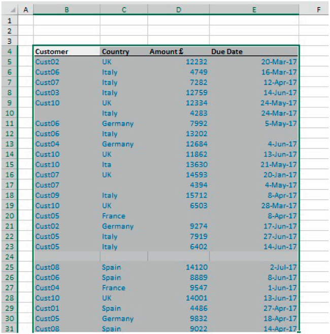
FIGURE 32.5 A Selected Data Set Before the Delete Blank Rows Code is Run
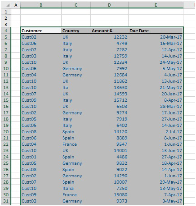
FIGURE 32.6 The Data Set After the Delete Blank Rows Code Has Run
Example: Deleting Blank Rows
In the above example, the range in which rows were to be deleted was pre-selected by the user. A more automated procedure would be to invoke the .UsedRange property of a worksheet. When doing this, one needs to take into account that the simultaneous deletion of multiple rows may not be permissible, and that when a single row is deleted, those that are below it are moved up in Excel; as a result, one needs to work backwards from the bottom of the range to delete the blank rows.
The file Ch32.9.DaysLateAnalysis.DeleteRows2.xlsm contains an example of this, using the following code:
With ActiveSheetNRows = .UsedRange.Rows.CountFor i = NRows To 1 Step -1 ' need to work backwards else may get empty rowsSet myRow = Rows(i).EntireRowNUsedCells = Application.WorksheetFunction.CountA(myRow)If NUsedCells = 0 ThenmyRow.DeleteElseEnd IfNext i
Figure 32.7 shows an original data set to which this is applied, and Figure 32.8 shows the result. Note that blank rows at the top of the worksheet were removed, but also that rows in which not all cells are blank are not deleted.
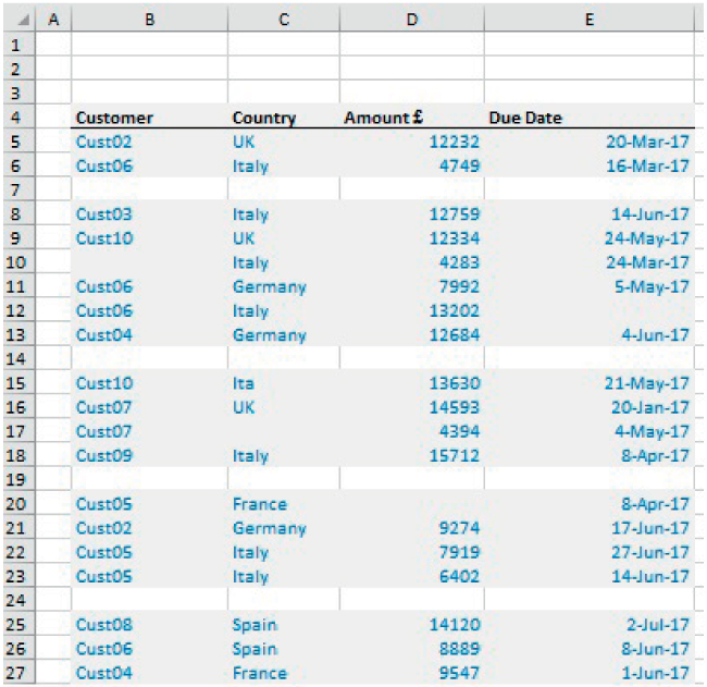
FIGURE 32.7 Deleting All Blank Rows in the Used Range: Before
FIGURE 32.8 Deleting All Blank Rows in the Used Range: After
The above two examples could be used in sequence to remove all rows which are either blank, or for which one of the data entries is blank (even if the row is not entirely blank).
Example: Automating the Use of Filters to Remove Blanks or Other Specified Items
In some cases, the items that one may wish to remove when cleaning or tidying a data set may not be those containing blanks, but those that have some other form of identifier (including blanks as one case). In Chapter 26, we showed the use of Excel's Data/Filter and Data/Advanced Filter to perform such operations on a one-off basis. It is relatively straightforward to record and appropriately adapt a macro of such operations. Recall that the main steps in the process that would initially be recorded are:
- Applying a filter to identify and select the items that one wishes to delete.
- Selecting the full range of filtered rows.
- Deleting these rows in the usual way (i.e. using Home/Delete Cells or right-clicking to obtain the context-sensitive menu).
- Removing the filters.
The file Ch32.10.DaysLateAnalysis.DeleteUsingFilter.xlsm contains an example. Figure 32.9 shows an original data set (assumed to be contiguous for the moment). One could then record the above steps, for example where one removes either blanks or the entries associated with Italy (from the Country field). If one initially records the above steps, except for the deletion process (i.e. those of selecting the data set, applying a filter and then removing the filter), one would have code such as:
Sub Macro1()Range("B4").SelectSelection.CurrentRegion.SelectSelection.AutoFilterActiveSheet.Range("$B$4:$E$104").AutoFilter Field:=2, Criteria1:="="ActiveSheet.Range("$B$4:$E$104").AutoFilter Field:=2, Criteria1:="Italy"ActiveSheet.ShowAllDataEnd Sub
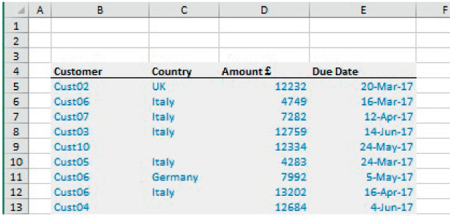
FIGURE 32.9 Original Data Set Before Application of the Procedure
Note that for reference purposes regarding the syntax, when recording the code, the filter on the Country field was first applied to blanks and then applied to Italy.
When developing a more general macro, one would likely wish to include additional elements such as:
- Specifying the value of the field that is of interest for deletion (e.g. blank rows or those associated with Italy), including ensuring that the filter is applied to the correct column Field. For example, one may instead wish to delete all blanks or all entries associated with Cust07 in the Customer field.
- Deleting the filtered rows, except for the headings.
The following points about the sample code below are worth noting:
- The
Application.InputBoxis used to take a cell reference from the user, whose contents identifies the item that define the items to be deleted. - With reference to this cell, the field column number associated within this identifier is calculated (i.e. equivalent to
Field:=2) in the above example, noting that this column field number is its relative position within the data set. - The filter is then applied, and a range created that contains all filtered data, except for the header.
- In practice, one may wish to switch on/off the screen updating (see Chapter 30), especially if such operations were to be further automated within a large loop that deletes a large set of records, according to pre-defined identifiers (this is not shown within the text of the code for simplicity of presentation).
Sub MRWrittenFilter()Set CelltoSearch = Application.InputBox("Click on cell containing the identifier data to delete", Type:=8)With CelltoSearchidItemtoDelete = .TextSet DataAll = .CurrentRegionicolN = .Column - DataAll.Cells(1, 1).Column + 1End WithDataAll.AutoFilter Field:=icolN, Criteria1:=idItemtoDeleteSet DataAll = DataAll.CurrentRegion.Offset(1, 0)DataAll.EntireRow.DeleteActiveSheet.ShowAllDataEnd Sub
The code could be modified so that it works for non-contiguous ranges of data (using.UsedRange rather than .CurrentRegion). In this case, one would generally first delete all rows that are completely blank (using the method outlined in the earlier example), before deleting filtered rows according to the user input (as shown in the earlier part of this example). Thus, one could have two separate subroutines that are each called from a master routine; the following code is also contained within the file:
Sub MRClearBlankRowsANDIdRows()Call MRDeleteBlankRowsCall MRDeleteIdRowsEnd SubSub MRDeleteBlankRows()'/// DELETE ALL COMPLETELY BLANK ROWSWith ActiveSheetSet DataAll = .UsedRangeNRows = DataAll.Rows.CountFor i = NRows To 1 Step -1Set myRow = Rows(i).EntireRowNUsedCells = Application.WorksheetFunction.CountA(myRow)If NUsedCells = 0 ThenmyRow.DeleteElseEnd IfNext iEnd WithEnd SubSub MRDeleteIdRows()'/// DELETE BASED ON USER INPUTWith ActiveSheetSet DataAll = .UsedRangeSet CelltoSearch = Application.InputBox("Click on cell containing the identifier data to delete", Type:=8)With CelltoSearchidItemtoDelete = .TexticolN = .Column - DataAll.Cells(1, 1).Column + 1End WithDataAll.AutoFilter Field:=icolN, Criteria1:=idItemtoDeleteSet DataAll = DataAll.CurrentRegion.Offset(1, 0)DataAll.EntireRow.DeleteActiveSheet.ShowAllDataEnd WithEnd Sub
Finally, note that there are many possible variations and generalisations of the above that would be possible, such as:
- Removing items based on multiple identifiers, by specifying these identifiers within a range and then working through all elements of that range (rather than using a user input box for each item).
- Copying the items to a separate area (such as a new worksheet that is automatically added using the techniques discussed earlier) before deleting the records from the main data set, thus creating two data sets (i.e. a main clean data set, and another containing the items that have been excluded). In practice, the data set of excluded items may define a set of items for which the data records need further manual investigation, before reinclusion in the main data set.
- Extracting or deleting items based on a Criteria Range and Advanced Filters.
The experimentation with such generalisations is left to the reader.
Example: Performing Multiple Database Queries
We noted in Chapter 26 that, when trying to perform multiple queries using Database functions one was not able to use functions within the Criteria Range (to perform a lookup process), since blanks that are calculated within the Criteria Range are not treated as genuinely empty cells. The alternative was the repeated Copy/Paste/Value-type operations; clearly, these can be automated using VBA macros (using assignment statements within a Loop).
The file Ch32.11.DaysLateAnalysis.DatabaseFunctions3.MultiQuery.xlsm contains an example. Figure 32.10 shows a screen-clip of the criteria ranges and the results ranges (the database is in the left-hand columns of the file, not shown in the clip). The basic procedure (as indicated by the arrows) is to assign, into the Criteria Range, the values of the various queries that are to be run, to recalculate the Database functions, and to assign the results to storage area. To facilitate the writing and robustness of the code, the various header fields have been given named ranges within the Excel file (e.g. CritToTestHeader refers to the header of the range that list the set of criteria to be tested, and CritHeader refers to the header for the criteria range for the Database functions.)
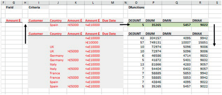
FIGURE 32.10 Results of Running a Set of Queries of Different Structures
The code to do this is:
Sub MRMultiQueries()Dim i As Long, N As LongWith DataSheetN = Range("CritToTestHeader").CurrentRegion.Rows.CountN = N - 1For i = 1 To NRange("CritHeader").Offset(1, 0).Value = _Range("CritToTestHeader").Offset(i, 0).ValueCalculateRange("ResultStoreHeader").Offset(i, 0).Value = _Range("Result").Offset(1, 0).ValueNext iEnd With
In a more general application, one would likely wish to clear the results range (but not its headers) at the beginning of the code run, using techniques discussed earlier; this is left as an exercise for the interested reader.
Example: Consolidating Data Sets That Are Split Across Various Worksheets or Workbooks
A useful application is the consolidation of data from several worksheets. In this example, we assume that the data that needs to be consolidated resides on worksheets whose Excel names each start with a similar identifier (such as Data.Field1, Data.Field2, with the identifier being the word Data in this case). Further, we assume that the column structure of the data set in each of these worksheets is the same (i.e. the database fields are the same in each data set, even as the number of row entries may be different, and perhaps the placement within each Excel data sheet may be different).
The file Ch32.12.DataConsol.xlsm contains an example. Figure 32.11 shows the worksheet structure of the file, which is intended to capture the more generic case in which:
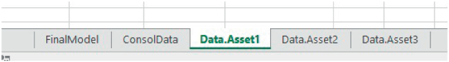
FIGURE 32.11 Generic Model Worksheet Structure
- There are multiple separate data worksheets.
- A macro is used to consolidate these into a single data set (in the ConsolData worksheet).
- The final model is built by using queries to this database (such as using SUMIFS functions) as well as other specific required calculations.
Figure 32.12 shows an example of the data set for Asset1, and Figure 32.13 shows the final consolidated data set.
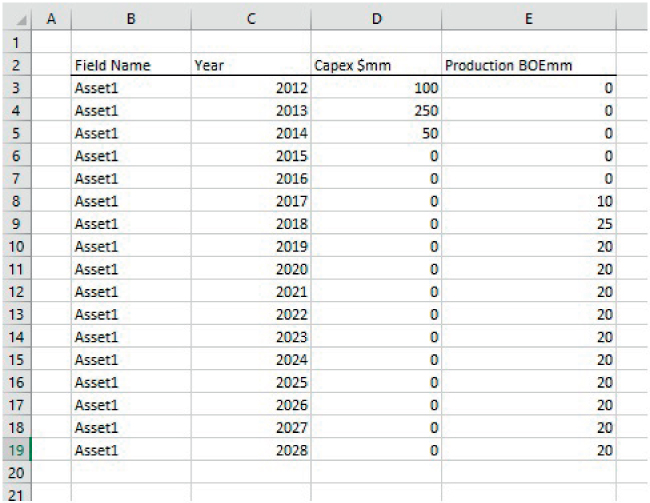
FIGURE 32.12 Example Data Set
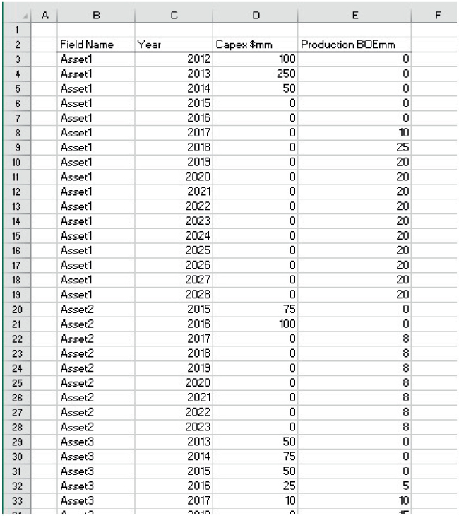
FIGURE 32.13 Final Consolidated Data
The following macro is contained within the file, and will consolidate the data sets together. The code works through the collection of worksheets in the workbook, and checks each worksheet's name to detect if it is a data sheet (as discussed earlier in this text):
- Where a data sheet is detected, it is activated and the size of the used range on that sheet is determined (the number of columns and the total number of points). The code implicitly assumes that the first row of the data contains headers that do not need copying (in fact, to make this code slightly simpler, we assume that the headers are already placed within the ConsolData worksheet). It then defines a range that contains all data except the headers, and counts the number of rows in this range.
- The ConsolData sheet is then activated and the number of rows that are already used in this range is counted (for example, when copying the second data set, one should not overwrite the data copied from the first data set). A new range is created whose size is the same as required to copy the data set that is currently being worked on, and whose position is such that it starts immediately below existing data. The values from the range in the data set are then assigned to the range in the ConsolData sheet.
- In general, this code would start with a call to another subroutine that clears out all data in the ConsolData sheet (apart from the headers). For clarity of presentation, this step has been left out of the code below, but its implementation simply requires using techniques covered earlier in the text.
Sub MRConsolFieldSheets()With ThisWorkbookFor Each ws In WorksheetsIf UCase(Left(ws.Name, 4)) = "DATA" Thenws.ActivateWith ActiveSheet.UsedRangeNCols = .Columns.Count 'number of columns in the user rangeNPts = .Count ' total number of cells in the used rangeSet startcelldata = .Cells(NCols + 1) ' 1st cell of second rowSet endcelldata = .Cells(NPts)Set rngToCopyFrom = Range(startcelldata, endcelldata)NRowsCopyFrom = rngToCopyFrom.Rows.CountEnd WithConsolDataSheet.ActivateWith ConsolDataSheetSet firstcell = .UsedRange.Cells(1)Set fulldata = firstcell.CurrentRegionNRowsExisting = fulldata.Rows.CountSet firstcellofPasteRange = firstcell.Offset(NRowsExisting, 0)Set endcellofPasteRange = firstcellofPasteRange.Offset(NRowsCopyFrom - 1, NCols - 1)Set rngTocopyTo = Range(firstcellofPasteRange, endcellofPasteRange)End WithrngTocopyTo.Value = rngToCopyFrom.ValueElse ' worksheet is not a DATA sheet'do nothingEnd IfNext wsEnd WithEnd Sub
Note that similar code can be written when the data sets are distributed across several workbooks that are contained in a separate data folder. Most of the principles of the code would be similar to above, although some additional techniques and syntaxes may be necessary, including:
- Being able to locate automatically the folder containing the data sets. Assuming that such a folders is called DataSets and is contained within a larger folder that includes the main workbook, this could be achieved with code such as:
strThisWkbPath = ThisWorkbook.PathstrDataFolder = strThisWkbPath & "" & "DataSets"
- Opening each workbook in turn, with code such as:
Workbooks.Open (strWkbToOpen)- Closing each workbook once the relevant data has been copied (or assigned), with code such as:
Workbooks(strFileNoExt).Close SaveChanges:=False(Doing so is left as an exercise for the interested reader.)