
CHAPTER 26
Filters, Database Functions and PivotTables
INTRODUCTION
This chapter discusses several Excel functions and functionalities that can assist in the analysis of data sets, including:
- Filter and Advanced Filters, which present or extract a filtered data set whose elements meet specific criteria.
- Database functions, which return calculations of the values in a database that meet certain criteria (without explicitly extracting the relevant data points), and whose results are live-linked to the data set. Although equivalent calculations can generally be conducted with regular Excel functions (such as SUMIFS or MAXIFS), the Database functions allow the identity of the criteria to be more rapidly changed. As functions, they generally require that errors or other specific values within the data set are corrected or explicitly dealt with through new criteria, to eliminate them from the calculation process.
- PivotTables, which create summary reports by category and cross-tabulations. Although not live-linked to the data set (so need refreshing if the data changes), PivotTables allow for very rapid reports to be created, for the identity of the criteria to be changed, and for rapid “drill-downs” or more detailed analysis of the data to be conducted very quickly. They also allow for errors or other specific values in the underlying data to be ignored (or filtered out) when applying the criteria or filters.
The chapter does not deal with the linking of Excel to external data sets, such as an Access database or SQL servers, or other options that are contained on the Data tab; such techniques are outside the scope of this text.
ISSUES COMMON TO WORKING WITH SETS OF DATA
Cleaning and Manipulating Source Data
In practice one will often have to manipulate or clean initial data before it can be used for analysis and reporting purposes. There are many techniques that may need to be applied in such cases, including:
- Splitting items into separate components using the Data/Text-to-Columns functionality or Excel functions (such as Text functions, see Chapter 23).
- Recombining or joining items based on finding (or creating) keys in one set that uniquely match with keys in another (see Chapter 23, Chapter 24 and Chapter 25 for many of the underlying techniques frequently required).
- Reversing or transposing data, using either Copy and Paste/PasteSpecial or functions (e.g. array or lookup functions, see Chapter 18 and Chapter 25).
- Identifying spelling mistakes or unclear identifiers. For example, it may be that a country name (such as Italy) is listed with multiple identifiers (such as Italy, Italie, Italia, Repubblica Italiana, or simply It). Similarly, there may be blanks or other unwanted items in the data set. Most of these can be identified by application of a Filter, followed by the inspection of the drop-down menu, which will list the unique values. Alternatively, the full column of data can be copied to a separate field and techniques such as Data/Remove Duplicates and/or a Data/Sort applied. One can also use Excel's Conditional Formatting options to highlight certain values, such as errors, duplicates, positive or negative items etc.
- Correcting spelling mistakes or unclear identifiers. This can be done either manually when there are only a few entries, or using operations such as Find/Replace.
- Deleting unwanted items. Some items, such as blank rows or entries that are not relevant for any analysis, may need to be deleted. This can be done manually if there are only a few items, or using Filters if there are more (see example below). In more extensive cases, the process can be largely automated using macros (see Chapter 32). An alternative to deleting unwanted items is to extract them; this may be achieved using the Advanced Filter functionality (see below).
- To identify the unique list of items within a category (such as country names and customers), or a unique list of combined items (such as unique country–customer combinations). Once again, the Data/Remove Duplicates functionality can be helpful in this respect.
Static or Dynamic Queries
In general when analysing data sets, one has two generic approaches to creating summary reports:
- Those which are fully live-linked to the data as well as to the criteria, i.e. as functions. The use of Database functions (or perhaps of regular Excel functions such as SUMIFS or MAXIFS) falls into this category, and is generally more appropriate where:
- The structure of a data set is essentially fixed and well understood, with little exploratory (“drill-down”) analysis required.
- The data values will be regularly updated, so that a dynamic calculation will automatically update with little or no rework.
- The identities of the criteria used are relatively stable and simple.
- The data contain few errors or, where errors are present, they can be easily (ideally automatically) identified, eliminated or handled appropriately.
- The reports form an interim step in a modelling process, with the results used to perform further calculations, and it is desired (from a modelling perspective) to have a full dynamic link from the underlying data through to the model results.
- Those which are numerical summaries of the data, but which are not fully live-linked. The use of Filters and PivotTables falls into this category. Such approaches are often appropriate where one intends to explore relationships between items, conduct drill-down analysis, change the criteria that are used to present a report, or otherwise alter the presentation of reports (e.g. change row into column presentations).
Creation of New Fields or Complex Filters?
When performing complex database queries (based on multiple underlying criteria or on unusual criteria), one has a choice as to whether to apply such criteria at the reporting level only (whilst leaving the data set unchanged), or whether to add a new calculated field to the data set, with such a field being used to identify whether the more complex set of criteria has been met (e.g. by producing a flag field that is 0 or 1, accordingly). This latter approach is often simpler and more transparent than creating a complex criteria combination at the query level. Of course, it increases the size of the data set, so that where many such combinations are required, it can be more efficient (or only possible) to build them within the reporting structure instead.
In some cases, a combined approach may be necessary. For example, if one of the criteria for a query were the length of the country name, or the third letter of the name, then it would likely be necessary to create a new field (e.g. using the LEN or MID functions) to create this field explicitly in the database.
Excel Databases and Tables
An Excel database is a contiguous range of cells in which each row contains data relating to properties of an item (e.g. date of birth, address, telephone number of people), with a set of column headers that identify the properties. The column structure of a database differentiates it from general Excel data sets, in which formulae may be applied to either rows or columns.
Note also that it is generally important for the field names (headers) to be in a single cell, and for a structured approach to be used to create them (especially for larger databases). The frequent approach in which categories and sub-categories are used to define headers using two or more rows is not generally the most appropriate approach. Rather, field headers will need to be in a single row. For example, instead of having one “header” row and a “sub-header” row beneath it, the headers and sub-header fields can be combined in a structured way. This is illustrated in Figure 26.1, in which the range B2:I3 contains the (inappropriate) two-row approach, and in Figure 26.2, where the range B3:I3 contains the adapted single-row approach.

FIGURE 26.1 Multiple Row Field Identifiers – To Be Avoided When Using Databases and Tables

FIGURE 26.2 Single Row Field Identifiers – To Be Preferred When Using Databases and Tables
An Excel Table is a database that has been explicitly defined as a Table, using any of:
- Insert/Table.
- Home/Format as Table.
- The short-cut Ctrl+T (or Ctrl+L).
During the process of creating a Table, there is a possibility to explicitly define a name for it; otherwise Excel will automatically assign one (such as Table1).
The key properties (and benefits) of Tables are:
- Data extension when a new data row is added in a contiguous row at the bottom of the data set. Any formula that refers to the table (using the Table-related functions and syntax) will automatically adapt to include the new data.
- Formulae extension when a formula is introduced into the first data cell of a new column; the formula is automatically copied down to all rows as soon as it is entered.
- Alternate-row colour formatting (by default) for ease of reading.
- The default naming based on a numerical index can facilitate the automation of some procedures when using VBA macros.
(Once a Table has been defined, it can be converted back to a range by right-clicking on it and using Table Tools/Convert to Range, or by using the Convert-to-Range button on the Design tab that appears when selecting any point in the table.)
Automation Using Macros
In many real-life applications, the techniques in this chapter (and general techniques in data manipulation and analysis) become much more effective when automated with VBA macros. For example:
- Although an individual (manually activated) filter can be applied to remove items with properties (such as blanks), a VBA routine that removes a specified item at the click of a button can be more effective when such repeated operations are required.
- To automate the process (at the click of a button) of producing a list of unique items for a field name (e.g. by automating the two manual steps of copying the data and removing duplicates).
- To explicitly extract many individual subsets of the data and place each one in a new worksheet or workbook.
- To perform multiple queries using Database functions for a set of criteria whose structure is changing (as calculated blanks or fields are not truly blank).
- Some databases may be generated using a single bank of formulae that is copied to individual cells by use of macros. The copying process may be done in stages, after each of which formula are replaced with values, to reduce memory space and computational intensity.
Examples of these techniques are discussed in Chapter 32.
PRACTICAL APPLICATIONS: FILTERS
Example: Applying Filters and Inspecting Data for Errors or Possible Corrections
Filters can be applied by simply selecting any cell in the database range and clicking on the Data/Filter icon. Note that when doing so it is important to ensure that the field headers are included (or the top row will by default be treated as containing the headers).
Further, one should define the data set within a single isolated range with (apart from the headers) no adjoining labels, and have no completely blank rows or columns within the intended data set. In this case, the default data set will be the Current Region of the selected point, i.e. the maximum-sized rectangular region defined by following all paths of contiguity from the original point. In practical terms, all rows above and below are included up to the point at which a first blank row is encountered (and similarly for columns), so that it is important to ensure that there are no blank rows in the data set, and that there are no additional labels immediately below the data set or above the field headings (and similarly in the column direction). Note that the Current Region of the selected point can rapidly be seen by using the short-cut Ctrl+Shift+*.
The file Ch26.1.DaysLateAnalysis.Initial.xlsx shows an example of a filter applied to a data set. Note that drop-down menus are automatically added to the headers, with these drop-downs providing sorting options as well as field-sensitive filtering options. The list of filtering options for a given field (e.g. for the Country field) provides the ability to quickly inspect for errors (e.g. spelling errors, or negative numbers in contexts where all numbers should be positive, as well as see whether blank items are present). Figure 26.3 shows an example of the initial data set, and Figure 26.4 shows the results of applying, within the Country field, the filters to select only the blanks or incorrect spelling of the country Italy.

FIGURE 26.3 Part of an Initial Data Set Before Correcting for Spelling Mistakes or Blanks
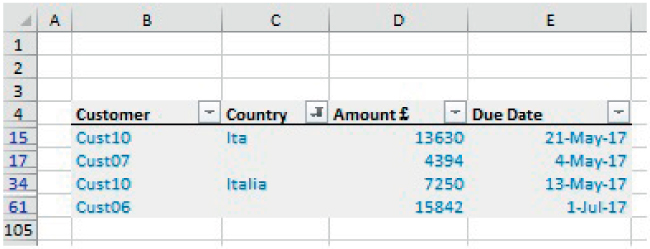
FIGURE 26.4 Data Filtered to Show Only Incorrect or Blank Entries Within the Country Field
Note that potential disadvantages of this standard filter approach are that:
- The criteria used to filter the data set are embedded within the drop-down menus and are therefore not explicit unless one inspects the filters.
- For data sets with many columns, it is not always easy to see which filters have been applied.
An easy way to remove all filters is with the short-cut Alt-D-F-S.
Note that one needs to take extra care when applying most Excel functions to a filtered data set, as the results may be unexpected or not intuitive. For example, for most regular Excel functions (e.g. SUM, COUNT), the result is the same whether the data is visible or not and whether it is filtered or not. On the other hand, the SUBTOTAL function has options to include or ignore hidden data (see Chapter 17), but these options may have unexpected effects when the data is filtered. Once a filter is applied, a row that is hidden (either before or after the application of the filter) is treated as if it were filtered out (rather than being not filtered out but simply hidden).
Figure 26.5 shows the functions applied to a filtered data set, and Figure 13.6 shows the same, except that one of the rows has been hidden. Within each case, the SUBTOTAL function returns the same result, which is that based on the visible data, so that the function options regarding hidden data seem to have no effect in Figure 26.6. The reader can verify in Excel file that with filters removed, the hiding of a row will lead to the two SUBTOTAL functions giving different results.
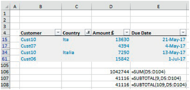
FIGURE 26.5 Functions Applied to a Filtered Data Set

FIGURE 26.6 Functions Applied to a Filtered Data Set with a Hidden Row
Thus, it is generally advisable not to apply Excel functions to filtered data. Rather, the use of Database functions or other approaches in which criteria are made explicit within the functions (such as using SUMIFS) are to be preferred.
Example: Identification of Unique Items and Unique Combinations
In order to analyse a data set, one may also need to identify the unique list of items within a category (such as country names and customers), or a unique list of combined items (such as unique country-customer combinations). The use of Excel's Remove Duplicates (on the Data tab) is an important functionality in this respect, enabling one to generate the actual list of unique items.
The file Ch26.2.DaysLateAnalysis.UniqueItems.xlsx shows an example. In the first step, one copies all the data in the relevant common (such as the country names) to another area not contiguous with the data set (perhaps using the short-cut Ctrl+Shift+↓ to select the data). The Remove Duplicates menu is then used to create a list of unique items (taking care as to whether the header field has been copied or not). Figure 26.7 shows the initial steps of this process, applying the Remove Duplicates to the copied set of Country data, with the result shown in Figure 26.8.

FIGURE 26.7 Applying Remove Duplicates to Copied Data

FIGURE 26.8 Unique Items Resulting from Application of Remove Duplicates
The identification of unique combinations can be done in one of two ways:
- Creating a text field which combines (joins or concatenates) these items (as discussed in Chapter 12), and use Remove Duplicates on the field of combined items.
- Using the Remove Duplicate menu applied to the copied data set of the two fields.
The file Ch26.3.DaysLateAnalysis.UniqueCombinations.xlsx shows the results of using the second approach. Figure 26.9 shows the initial steps in its application (i.e. the copying of the relevant data sets and application of the Remove Duplicated menu). Note that if working with a larger data set (such as if the whole data set had been copied so that the columns for the date or amount would not be relevant for the definition of unique items), the check-boxes that show within the Remove Duplicates dialog for these items would simply be left unticked. Figure 26.10 shows the result of the process.

FIGURE 26.9 Application of Remove Duplicates to Identify All Unique Combinations

FIGURE 26.10 Unique Combinations Resulting from Application of Remove Duplicates
Example: Using Filters to Remove Blanks or Other Specified Items
When cleaning or tidying data sets, one may wish to simply delete some rows, including:
- Where data is incomplete.
- Where there are errors.
- Where other specific items are not relevant or desired (such as all entries for the country Italy).
- Where there are blank rows.
As noted above, the use of the short-cut Ctrl+Shift+* to select the data would not select anything below the first blank row, so that if the presence of blank rows within the data set is possible, this shortcut should not be used; rather, the data set should be selected explicitly in its entirety before applying filters.
The file Ch26.4.DaysLateAnalysis.DeleteUsingFilter.xlsx shows an example. The main steps in are:
- Apply a filter to identify and select the items that one wishes to delete (generally, it is worth keeping a copy of the original data set, in case mistakes arise during some part of the process and steps need to be redone).
- Select the full range of filtered rows (this can be done in the usual way, as if selecting a contiguous range of cells, even if the cells are in fact not contiguous).
- Delete these rows in the usual way (i.e. using Home/Delete Cells or right-clicking to obtain the context-sensitive menu).
- Remove the filters.
Let us assume that it is desired to remove all records for which the Country field is either blank or applies to Italy (which are assumed to both be regarded as irrelevant for all subsequent analysis purposes). Figure 26.11 shows the part of the process which has filtered the data, and has selected the filter rows in preparation for their deletion. Figure 26.12 shows the result when these rows have been deleted and the filters removed, thus giving the cleaned data set.

FIGURE 26.11 Filtering and Selecting of Rows Which Are Desired to be Deleted

FIGURE 26.12 Result of Deleting Specified Rows
Note that this process can be automated relatively easily with VBA macros. For example, when the macro is run, the user could be asked to click on a specific cell which contains the identifier of the items to be deleted within that field (e.g. a blank cell, or a cell containing the word Italy), with the macro taking care of all other steps behind the scenes. In this way, data sets can be rapidly cleaned: the copying, filtering and removal of filters is embedded as part of the overall process, and one can run such a process many times very quickly.
Example: Extraction of Data Using Filters
In some cases, one may wish to use filters to extract items rather than to delete them. In such a case, the initial part of the process can be performed as above (up to that shown in Figure 26.11), whereas the latter part would involve copying the data to a new range, rather than deleting it. This is in principle a very straightforward and standard operation if basic Excel elements are respected (such as ensuring that any copy operation does not overwrite the original data). Note that Excel will replace any calculated items with their values to ensure integrity of the process.
Example: Adding Criteria Calculations to the Data Set
Although Excel provides several in-built options regarding filters, it is often more convenient to add a new criterion to the data set.
The file Ch26.5.DaysLateAnalysis.NewCriteria.xlsx shows an example in which it is desired to identify and delete all rows in which two or more field elements are blank. A new column has been added which uses the COUNTBLANK function to calculate the number of blanks fields (see Figure 26.13). For simplicity of presentation, Conditional Formatting has been applied to highlight those cells where the identified number of blanks in the row is equal to the threshold figure (defined in Cell F2). In other words, it identifies the rows that may be desired to be deleted. Note that (since the original data set in the example was not explicitly defined as an Excel table), once this column is added, the Data/Filter menu will need to be reapplied to ensure that a filter is included in the new column. The same procedure(s) as in the above examples can then be used to simply filter out and delete (or copy) these rows.

FIGURE 26.13 Addition of a New Field to Capture Specific or Complex Criteria
Example: Use of Tables
Generally, it is preferable to define the data set as an Excel Table. Note that one needs to take care to ensure that, if an original data set contains blank rows, then the Table range needs to be extended to include all data (as the Insert/Table operation will have selected only the Current Region of a data point by default).
The file Ch26.6.DaysLateAnalysis.Table1.xlsx shows an example of the process to create a Table (see Figure 26.14), noting that the default range would have been only up to Row 15 (as Row 16 is blank), so that the range was manually extended to include the rows up to Row 104.
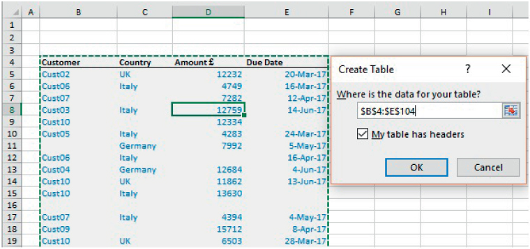
FIGURE 26.14 Defining the Data Range for a Table
Once defined as a Table, any (contiguous) new contiguous rows or columns that are added will automatically become part of the Table. In addition, a formula entered in the first data cell of a field will be copied to all rows of the table. Indeed, the simple making of entry in such a cell (such as in Cell F5 of the original, non-extended, Table) will result in a new column being added automatically. Figure 26.15 shows the same process as above (in which the COUNTBLANK function is used as a new field), when applied to a Table.

FIGURE 26.15 Addition of a New Column to a Table
Note that the syntax of the formula in every cell within the Table range of column F is the same (and is not row-dependent):
If one were to change the formula, such as to count the blanks from different points, then the deletion of the original field name (as shown Figure 26.16) will produce a drop-down menu of field names that can be chosen instead to build the required formula.

FIGURE 26.16 Modification of Formulae Using the Header Names Generated Within the Table
Note also that, when using a Table, one can create formulae using the Header Names that the Table generates, such as:
Finally, note also that when one has selected a cell within the Table, the Table Tools Design Tab appears. This contains icons to Remove Duplicates and to create a PivotTable summary. The tab also allows one to rename the Table, although experience suggests that this process is best done when the Table is first created, and not once formulae have been built that refer to the name.
Example: Extraction of Data Using Advanced Filters
In some earlier examples, we used the filtering process embedded within the drop-down menus both to delete unwanted data and to extract data that may be wanted for separate analysis. In practice, such approaches are generally most appropriate only for the deletion of data, whereas the extraction of wanted items to another range is more effectively implemented using the Data/Advanced Filter tool.
The file Ch26.7.DaysLateAnalysis.ExtractCriteriaRange.xlsx shows an example (see Figure 26.17). Note that there is a separate range to define the criteria for the extraction and another range in which to copy the extracted data (this latter range is optional; as per the dialog box, the list can otherwise be filtered in place, so that the original full data set would simply be filtered as if done with a drop-down menu).

FIGURE 26.17 Example of the Implementation of An Advanced Filter
Note that:
- The Criteria range consists of some headers and at least one row below that which is contiguous with the headers. When multiple items are entered in a (non-header) row, are treated as representing “And” criterion. If additional non-header rows are used, each row is treated as an “Or” criterion (i.e. the results of the criteria on one row are added to those of the criteria on another); a frequent mistake is to include a blank row within the criteria range, which means that all elements would be included in the extraction or filter process.
- The header fields used in the Criteria range need to be identical to those of the main data set. If they are spelled even slightly differently, the process will not work as needed.
- For the Extract range, the headers are important only for cosmetic purposes; the extracted data set will be placed in the file in the same order as in the original data set, even if headers are not present in the Extract range. Of course, in practice, it is by far the most convenient to define the Extract range as that which contains a copy of the field headers (as in our example).
PRACTICAL APPLICATIONS: DATABASE FUNCTIONS
Excel's Database functions return calculations relating to a specified field in a database, when a set of criteria is applied to determine which records are to be included. The available functions are DAVERAGE, DCOUNT, DCOUNTA, DGET, DMIN, DMAX, DPRODUCT, DSTDEV, DSTDEVP, DSUM, DVAR and DVARP. For example, DSUM provides a conditional summation in the database, i.e. a summation of a field where only items that meet the defined criteria are included. In a sense, DSUM is similar to the SUMIFS function (similarly, DAVERAGE is similar to AVERAGEIFS, and DMIN or DMAX to MINIFS or MAXIFS). The other Database functions generally do not have simple conditional non-database equivalents (although the use of array functions does allow them to be reproduced in principle, as discussed in Chapter 18).
As for the Advanced Filter, Database functions require one to specify a Database (which may have been defined as an Excel Table), a Criteria Range (headers and at least one row, with additional contiguous rows representing OR criteria) and a field on which the conditional calculations are to be conducted.
Database functions and their non-database equivalents provide calculations which are dynamic or live-linked to the data set (in contrast to PivotTables). Each has advantages over the other:
- Non-database functions have the advantage that they work irrespective of whether the data is laid out in row or column form, and that they can be copied into contiguous rows (so that the functions can provide a set of values that relate to queries that involve different values of the same underlying criteria type, e.g. the sum of all items in the last month, or in the last two months etc.)
- Database functions require the data to be in column format. Their advantages include that they allow for the identity of the criteria to be changed very quickly: by entering values in the appropriate area of the criteria range, different criteria (not just different values for the same criteria) are being used. For example, one may wish to calculate the sum of all items in the last month, and then the sum of all items worth over £10,000, or all items relating to a specific country, and so on. When using the non-database equivalent (SUMIFS in this example), one would have to edit the function for each new query, to ensure that it is referencing the correct ranges in the data set and also in the criteria range. Note also that Database functions require the use of field header names (as do PivotTables), whereas non-database functions refer to the data set directly, with headers and labels being cosmetic items (as for most other Excel functions).
Example: Calculating Conditional Sums and Maxima Using DSUM and DMAX
The file Ch26.8.DaysLateAnalysis.DatabaseFunctions1.xlsx contains an example. Figure 26.18 shows part of a data set (which has been defined as a Table, and given the name DataSet1) as well as the additional parameter information required to use the Database functions, i.e. the name of the field which is to be analysed (in this case the field “Amount £”) and the Criteria Range (cells I4:L5). Figure 26.19 shows the implementation of some of the functions.

FIGURE 26.18 Database and Parameters Required to Use Database Functions

FIGURE 26.19 Implementation of Selected Database Functions
Example: Implementing a Between Query
If one wishes to implement a between-type query (e.g. sum all items whose amounts are between £5000 and £10,000), the simplest way is usually to extend the Criteria Range by adding a column and applying two tests to the same criteria field; this is analogous to the procedure when using a SUMIFS function, as discussed earlier in the text. (An alternative is to implement two separate queries and take the difference between them.)
The file Ch26.9.DaysLateAnalysis.DatabaseFunctions2.xlsx contains an example, which is essentially self-explanatory; Figure 26.20 shows the extended Criteria Range that could be used in this case.

FIGURE 26.20 Criteria Range Extended by a Column to Implement a Between Query
Example: Implementing Multiple Queries
When using Database functions, the Criteria Range consists of field headings and one or more contiguous rows below this. Thus, if a second set of criteria were required, a new Criteria Range would be needed, and if many such sets of criteria were required, there would be several such ranges, so that the space taken up in the workbook could become quite large (i.e. each Criteria Range would require at least three rows of Excel – the header, the criteria values and a blank row before the next Criteria Range).
An alternative is to have a single Criteria Range, and to place in sequence the set of values to be used for each query within this range, each time also recording the results of the query (as if doing a sensitivity analysis). Unfortunately, such a process cannot in general be simplified by using lookup functions to place the data within the criteria range: if the criteria range contains functions which return blank cells, then the Database functions do not consider such calculated blanks as being the same as if the cell containing the same criteria value were truly empty.
Thus, in practice, such a process needs to be done either manually or automated using VBA macros (see Chapter 32), because the copying in Excel (or assigning in VBA) of a blank cell into the Criteria Range leads to its value being treated as genuinely empty.
The file Ch26.10.DaysLateAnalysis.DatabaseFunctions3.xlsx shows examples of these. Figure 26.21 shows that the Database functions will return zero (cells O5:R5) when a lookup process is used to find the desired value to be used in the criteria range, even when the additional step is built, in that when blanks within the input ranges are referred to, the return values are also set to blank, not as zeros; see the Formula Bar. Since calculated blanks within the Criteria Range are not treated as if they were simple empty cells, no matching records are found. However, when the queries are pasted individually into the Criteria Range (for demonstration purposes, a new range has been set up in cells I8:M9), no such issue arises. One can repeat the process to copy the individual queries and each time paste the results into a storage range; in the Figure, the first three criteria sets have been completed, with the results pasted in cells O13:O15). Clearly, such a process can be automated using a VBA macro, as discussed in Chapter 32.
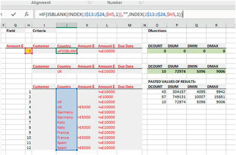
FIGURE 26.21 Database Functions Do Not Treat Calculated Blanks as True Blanks
PRACTICAL APPLICATIONS: PIVOTTABLES
PivotTables can be used to produce cross-tabulation reports which summarise aspects of a database by category. Their main advantages include:
- They allow to create reports very rapidly, for the identity of the criteria to be changed, and for “drill-downs” or more detailed analysis of the data to be conducted easily and quickly.
- The presentation of the report can easily be changed, e.g. switching rows and columns or reporting an average instead of a total. Further, additional filters and “slicers” can be added or removed, which can allow for very rapid exploration and analysis.
- They also allow for errors or other specific values in the underlying data to be ignored (or filtered out) when applying the criteria or filters.
- PivotCharts are easy to create from a PivotTable.
- They are supported by VBA, so that one can record macros based on actions applied to a PivotTable, and adapt these as required.
Despite their power, PivotTables have some properties which can be potential disadvantages:
- They are not live-linked to the data set, so need refreshing if the data changes. (This is because they use a “cache” of the original data. In fact, multiple PivotTables can be created using the same underlying data, and this should ideally be done by copying the first PivotTable to ensure that the same cached data is used and so not diminish computation efficiency when dealing with large data sets.)
- They will “break”, and will need to be rebuilt, if field headings change. For example, a PivotTable based on a field heading “2016 Salaries” would need to be rebuilt if – during an annual update process – the field header changed to “2017 Salaries”. This contrasts with regular (non-database) Excel functions (which are linked only to the data, with the field labels being essentially cosmetic), and to Database functions (which if implemented correctly do not break if field headings change, or at least require only minimal re-work). Thus, they may not be the most effective reporting methods for complex queries that will regularly be updated.
- Since the structure of the PivotTable (e.g. row–column layout, number of rows etc.) depends on the underlying data, it is generally not appropriate to use these as an interim calculation step (i.e. Excel formulae should generally avoid referencing cells in a PivotTable). PivotTables are thus best used both for general exploratory analysis, and as a form of final report.
Example: Exploring Summary Values of Data Sets
The file Ch26.11.DaysLateAnalysis.PivotTable1.xlsx shows an example of a simple PivotTable. The underlying database has been defined as an Excel Table called DataSet1 (although doing so is not necessary to create a PivotTable). The PivotTable was created by selecting any cell in the database and using Insert/PivotTable, and then filling in the data or choices required by the dialog box. When doing so, one may in general choose to place the PivotTable on a new worksheet to keep the data separate from the analysis, and to allow adaptation of the data set (insertion of new rows) without potentially causing conflicts. Figure 26.22 shows the foundation structure that is created automatically.

FIGURE 26.22 Foundation Structure of a PivotTable
Thereafter, the user can select field names using the check boxes and drag these to the Rows, Columns, Values or Filters areas, as desired. Figure 26.23 shows an example report which summarises the figures by country and customer.

FIGURE 26.23 Creation of PivotTable Row–column and Reporting Structure
Note that the report would simply be transposed if the items row–column structure of the country and customer were switched.
Figure 26.24 shows how one may choose to use a filter approach to present the results. In this example, the Country field was moved from the Columns are to the Filters area with the result that a new filter appeared in Row 1; this has been applied to show only the data relating to Germany.
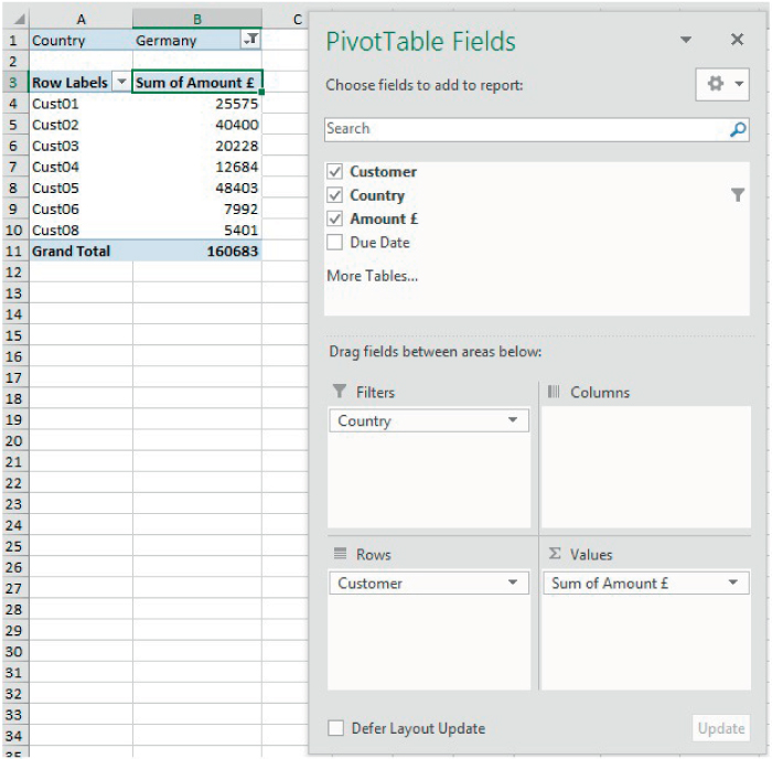
FIGURE 26.24 Basic Use of a Filter
Some additional important points include:
- Items can be re-ordered within the presentation using the Sort options, or manually by either right-clicking on an item and using the context-sensitive (Move) menu, or by simply clicking on the border of the cell containing the label and dragging this cell to the desired location.
- The PivotTable Tools/Analyze tab provides a wide range of options, including the use of the Field Settings to display calculations other than the sum totals, as well as the use of customised calculations.
- A second PivotTable (based on the same data cache) can be created either by using the More Tables option in the PivotTable Fields dialog, or by choosing Entire PivotTable within the Select option on the PivotTable Tools/Analyze tab, and then using a standard Copy/Paste operation. A PivotTable can be deleted by the same selection process and then using Excel's regular Clear Contents menu.
Figure 26.25 shows an example in which some of these points have been implemented: a second PivotTable has been inserted, a Filter is used in place of a column structure, and the order of the countries has been manually changed. Note that the PivotTable Fields dialog appears only once but is specific to the PivotTable that is active.

FIGURE 26.25 Representation of Report Based on a Copied PivotTable
Example: Exploring Underlying Elements of the Summary Items
An important feature of PivotTables is the ability to rapidly see the individual items that make up the summarised figure, i.e. to list the relevant detailed individual records in the underlying database. One can create such a list either by:
- Double-clicking on the cell in the PivotTable.
- Right-clicking and using Show Details.
Figure 26.26 shows the result of applying this process to Cell B23 (summary data for France) in the above example (shown in the DrillDown worksheet of the example file).
FIGURE 26.26 Example of Results of Drill-down of An Item in a PivotTable
Example: Adding Slicers
In their basic form, Slicers are rather like Filters, but simply provide an enhanced visual display, as well as more flexibility to rapidly experiment with options.
Slicers can be created using the menu on the PivotTable Tools/Analyze tab. Figure 26.27 shows an example of adding a Slicer on the Country field of the second PivotTable, and then showing the summary results for the selected set of countries (holding the Ctrl key to select multiple items).

FIGURE 26.27 Use of a Single Slicer
In Figure 26.28, we show the result of including a second Slicer (based on Customer), in which all items for the second Slicer are selected. Figure 26.29 shows the result of using the second Slicer to report only the items that relate to the customer Cust01; one sees that the Country slicer adjusts to show that such a customer is not present in Italy. This highlights one of the main advantages of slicers over filter approaches (i.e. reflecting correctly the interactions between subsets of the data).

FIGURE 26.28 Inclusion of a Second Slicer

FIGURE 26.29 Interactions Between the Slicers
Example: Timeline Slicers
Timeline Slicers are simply a special form of slicer that can be used (inserted using the PivotTable Tools/Analyze tab) when a date field is to be analysed. Rather than have to adapt the data (such as by using the MONTH or YEAR functions), the slicers automatically provide options to analyse the data according to different levels of time granularity. Figure 26.30 shows the result of inserting a TimeLine Slicer (in which the full Customer list is used), with the drop-down menu of the slicer set to the “Months” option.

FIGURE 26.30 Use of a TimeLine Slicer
Example: Generating Reports Which Ignore Errors or Other Specified Items
One useful feature of PivotTables is the ability to rapidly include or exclude data from the summary reports (using either filters or slicers). For example, a comment field within the data set may indicate that some items need to be treated in a special way.
The file Ch26.12.DaysLateAnalysis.PivotTable2.xslx shows an example. Figure 26.31 shows a database in which there is a comment field. Figure 26.32 shows a PivotTable in which a Slicer has been introduced, with the analysis intended to include only those items in the comment field that are either blank or marked “OK” or marked “Checked”.

FIGURE 26.31 Data Set with a Comment Field
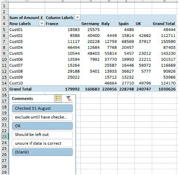
FIGURE 26.32 Using Slicers to Exclude Specific Commented Items
Note that if one were to conduct such summary analysis using functions (database or non-database), the bespoke treatment of such “corrected” items would be much more cumbersome: for example, one would generally need to create a special field in the database that acts as a criterion to determine whether items would be included or not in the calculation. However, since the comments made could essentially be anything, it could be quite cumbersome, time-consuming and error-prone to create the applicable formulae.
Example: Using the GETPIVOTDATA Functions
One can obtain (or lookup) a value in any visible PivotTable using the GETPIVOTDATA function. The function has a number of parameters:
- The name of the data field (enclosed in quotation marks).
- The Pivot_table argument, which must provide a reference to any cell in the PivotTable from which data is desired to be retrieved (or a range of cells, or a named range).
- The field and item names: these are optional arguments, and there could be several, depending on the granularity and number of variables in the PivotTable.
The file Ch26.13.DaysLateAnalysis.PivotTable3.xslx contains an example, shown in Figure 26.33.

FIGURE 26.33 Use of the GETPIVOTDATA Function
Since the data must already be visible, one might ask as to the benefit of this. One case where it may be useful is if there are many large PivotTables, but one wishes only selected data from them. In such cases, it may be that functions such as SUMIFS would be more appropriate (which may often be the case, unless the filter and slicer functionality is required simultaneously).
Example: Creating PivotCharts
Once a PivotTable has been created, a PivotChart can also be added using the PivotChart icon on the Analyze tab of the PivotTable Tools. The two objects are then inherently linked: the application of a filter on one will adjust the corresponding filter on the other, and the insertion of a slicer will affect both.
The file Ch26.14.DaysLateAnalysis.PivotTable4.xslx contains an example. Figure 26.34 shows a PivotChart in which a country filter is applied, and the column format of the PivotTable adjusts automatically. The Timeline slicer that has been inserted for the PivotTable also affects the display shown on the chart.
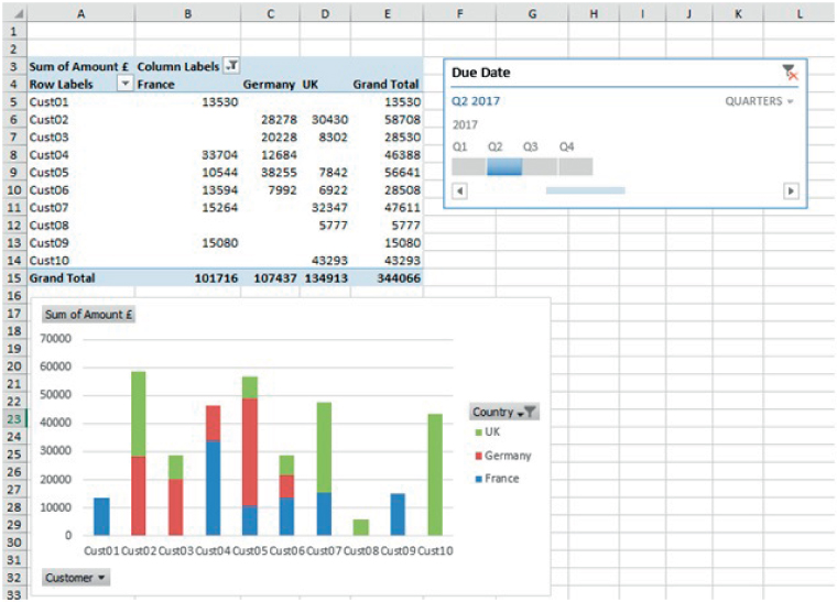
FIGURE 26.34 Example of a Pivot Chart and Alignment of Filters with Its PivotTable
Example: Using the Excel Data Model to Link Tables
Where one wishes to produce reports based on multiple databases or tables, it may be cumbersome to have to consolidate them together into a single database. Excel's Data Model allows for PivotTable analysis of multiple data sets by linking them through relationships (of course, one would still need to have, or to create, some form of identifier or key that enables the matching process to take place through the relationship, but the cumbersome and memory-intensive lookup functions can often be avoided).
The file Ch26.15.DataModel.xlsx shows an example. Figure 26.35 shows three data sets that have been defined as Excel Tables, with the first providing a complete list of unique identifiers for each customer, the second providing information on revenues and dates, and the third providing cost information.
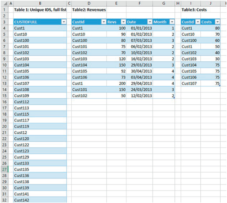
FIGURE 26.35 Data Sets Used for PowerView Example
To create a PivotTable report that uses information from these tables (without explicitly joining them into a single data set), the following steps are necessary:
- Define each data set as an Excel Table (see earlier).
- On the Data tab, use the Connections icon to add each Table in turn to the DataModel. This is done by using the drop-down from the Add menu to find AddtotheDataModel (see Figure 26.36), and selecting the Tables tab. When complete, the list of connections will be shown as in Figure 26.37.
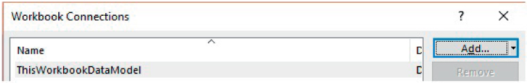
FIGURE 26.36 Adding a New Workbook Connection I
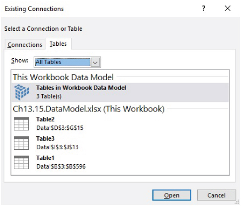
FIGURE 26.37 Completed List of Connections
- Define the relationships using Data/Relationships/New. In this example, the CUSTIDFULL field from the first table acts as the Primary Key (see Figure 26.38).

FIGURE 26.38 Defining Relationships Between the Tables
- Finally, create the PivotTable by using Insert/PivotTable. When doing so, one will need to check the “Use an external data source” within the dialog box, and choose “Tables in Workbook Data Model”. Figure 26.39 shows an example report.
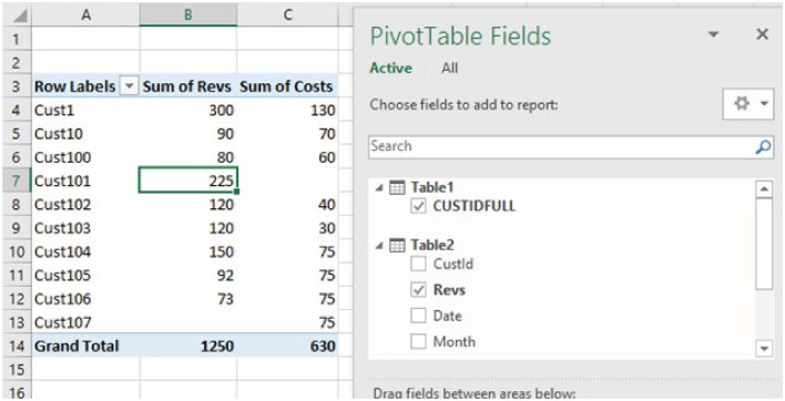
FIGURE 26.39 PivotTable Report Based on the DataModel