CHAPTER 15
Introduction to Simulation and Optimisation
INTRODUCTION
This chapter introduces the topics of simulation (with a more complete discussion being the subject of Chapter 16). It also extends the earlier discussion of optimisation. These are both natural extensions of sensitivity and scenario analysis. The first section discusses the link between these methods, and uses a practical example to illustrate the discussion. The latter sections of the chapter highlight some additional points that relate to general applications of optimisation modelling.
THE LINKS BETWEEN SENSITIVITY AND SCENARIO ANALYSIS, SIMULATION AND OPTIMISATION
Simulation and optimisation techniques are in effect special cases of sensitivity or scenario analysis, and can in principle be applied to any model which is built appropriately. The specific characteristics are that:
- Several inputs are varied simultaneously. As a result, combinatorial effects are important, i.e. there are many possible input combinations and corresponding output values.
- There is an explicit distinction between controllability and non-controllability of the process by which inputs vary.
These points are described in more detail below.
The Combinatorial Effects of Multiple Possible Input Values
When models contain several inputs that may each take several possible values, the number of possible input combinations generally becomes quite large (and hence so does the number of possible values for the model's output). For example, if 10 inputs could each take one of three possible values, there would be 310 (or 59,049) possible combinations: the first input can take any of three values, for each of which the second can take any of three values, giving nine possible combinations of the first two inputs, 27 for the first three inputs, and so on.
In practice, one needs automated methods to calculate (a reasonably large subset of) the possible combinations. For example, whereas traditional sensitivity and scenario analysis involves pre-defining the values that are to be used, simulation and optimisation (generally) automate the process by which such values are chosen. Naturally, for simulation methods, the nature of this automation process is different to that for optimisation, as described later.
Controllable Versus Non-controllable: Choice Versus Uncertainty of Input Values
The use of traditional sensitivity and scenario analysis simply requires that the model is valid as its input values are changed in combination. This does not require one to consider (or define) whether – in the real-life situation – the process by which an input value would change is one which can be controlled or not. For example, if a company has to accept the prevailing market price for a commodity (such as if one purchases oil on the spot market), then such a price is not controllable (and hence likely to be uncertain). On the other hand, the company may be able to decide at what price to sell its own product (considering that a high price would reduce sales volume and a lower price would increase it), and hence the price-setting is a controllable process or choice. In other words, where the value of an input variable can be fully controlled, then its value is a choice, so that the question arises as to which choice is best (from the perspective of the analyst or relevant decision-maker). Where the value cannot be controlled, one is faced with uncertainty or risk. Thus, there are two generic sub-categories of sensitivity analysis:
- Optimisation context or focus, where the input values are fully controllable within that context, and should be chosen optimally.
- Risk or uncertainty context or focus, where the inputs are not controllable within any specific modelled context. (Subtly, the context in which one chooses to operate is an optimisation issue, as discussed later.)
These are illustrated in Figure 15.1.
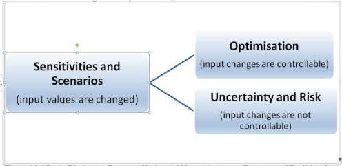
FIGURE 15.1 Basic Distinction Between Choice and Uncertainty as an Extension of Traditional Sensitivities
Of course, the distinction between whether one is faced with a situation in which there is uncertainty versus one of choice may depend one's perspective and role in a given situation. For example, it may be an individual's choice as to what time to plan to arise in the morning on a particular day, whereas from the perspective of someone else, the time at which the other person rises may be considered to be uncertain.
PRACTICAL EXAMPLE: A PORTFOLIO OF PROJECTS
Description
The file Ch15.1.TimeFlex.Risk.Opt.xlsx (see Figure 15.2) contains an example of a portfolio of 10 projects, with the cash flow profile of each being shown on a generic time axis (i.e. an investment followed by a positive cash flow from the date that each project is launched). Another grid shows the effect when each project is given a specific start date, defined in the range C15:C24, and which can be changed to be any set of integers (the model's calculations use lookup and other functions which the reader can inspect). In the case shown, all projects start in 2018, resulting in a portfolio with a net present value (NPV) of $1212m for the first 10 years' cash flows at a 10% discount rate, whilst the maximum financing requirement in any given year is $2270m (Cell D25).

FIGURE 15.2 Variable Launch Dates for Each Project Within a Portfolio
As mentioned earlier, the role of the various launch dates of the projects could depend on the situation:
- An optimisation context, in which the start dates are entirely within the discretion and control of the decision-maker, and can be chosen in the way that is the most suitable from the perspective of the decision-maker.
- A risk or uncertainty context, in which each project would be launched according to some timetable that is not within the decision-scope of the users of the model. Thus, each project is subject to uncertainty on its timing, so that the future cash flow and financing profile is also uncertain.
Optimisation Context
As an optimisation issue, one may wish to maximise the NPV over the first 10 years, whilst not investing more than a specified amount in each individual year. For example, if one considers that the total cash flow in any of the first five periods (net of investment) should not drop to below (minus) $500m, then the case shown in Figure 15.2 would not be acceptable as a set of launch dates (since the cash flow in 2018 is (minus) $2,270). On the other hand, delaying some projects would reduce the investment requirement in the first period, but would also reduce NPV. Thus, a solution may be sought which optimises this trade-off.
The file Ch15.2.TimeFlex.Risk.Opt.Solver.xlsx (see Figure 15.3) contains an alternative set of launch dates, determined by applying Solver, in which some projects start later than 2018. This is an acceptable set of dates, as the value in Cell C28 is larger than that in C29. Whilst it is possible that this set of dates is the best one that could be achieved, there may be an even better set. (Note that in a continuous linear situation, an optimal solution would meet the constraints exactly, whereas in this case, the input values are discrete integers, so that the constraints would be respected, but not necessarily met exactly.)
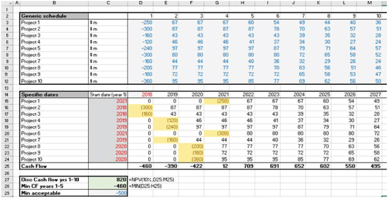
FIGURE 15.3 Using Solver to Determine Optimal Start Dates
Risk or Uncertainty Context Using Simulation
As a risk or uncertainty issue, the same model would apply if the project start dates were uncertain, driven by items that are not known or not within the control of the modeller or user.
Of course, given the large possible number of combinations for the start dates, whilst one could define and run a few scenarios, it would be more practical to have an automated way to generate all or many of the possible scenarios. Monte Carlo Simulation is an automated process to recalculate a model many times as its inputs are simultaneously randomly sampled. In the case of the example under discussion, one could replace the start dates with values that are drawn randomly in order to sample future year numbers (as integers), do so many times and record the results.
Figure 15.4 shows an example of the part of the model concerning the time-specific cash flow profile in one random scenario. Each possible start date is chosen randomly but equally (and independently to the others) from the set 2018, 2019, 2020, 2021 and 2022.

FIGURE 15.4 A Random Scenario for Project Start Dates and its Implications for the Calculations
Clearly, each random sample of input values would give a different value for the output of the model (i.e. the cash flow time profile, the investment amount and the NPV), so that the output of the simulation process is a set of values (for each model output) that could be represented as a frequency distribution. Figure 15.5 shows the results of doing this and running 5000 random samples with the Excel add-in @RISK (as discussed in Chapter 16 and Chapter 33, such calculations can also be done with VBA, but add-ins can have several advantages, including the ease with which high-quality graphs of the results can be generated).

FIGURE 15.5 Distribution of NPV that Results from the Simulation
Note that often – even if the variation of each input is uniform – the profile of an output will typically have a central tendency, simply because cases where all inputs are chosen at the high end of their range (or all are chosen at their low end) are less frequent than mixed cases (in which some are at the high end and others are at the low end). In other words, the need to use frequency distributions to describe the range and likelihood of output values is an inevitable result of the combinatorial effect arising due to the simultaneous variation of several inputs.
Note also that, within the earlier optimisation context, one may try to use simulation to search for the solution to the optimisation situation, by choosing the input combination that gives the best output; in practice, this is usually computationally inefficient, not least as the constraints are unlikely to be met unless a specific algorithm has been used to enforce this. This also highlights that simulation is not the same as risk modelling: simulation is a tool that may be applied to contexts of risk/uncertainty, as well as to other contexts. Similarly, there are other methods to model risks that do not involve simulation (such as using the Black–Scholes formula, binomial trees and many other numerical methods that are beyond the scope of this text).
FURTHER ASPECTS OF OPTIMISATION MODELLING
Structural Choices
Although we have presented optimisation situations as ones that are driven by large numbers of possibilities for input values, a specific objective, and constraints (i.e. combinatorial-driven optimisation), the topic also arises when one is faced with choices between structurally different situations, i.e. ones that each involve a different logic structure. For example:
- One may consider the decision as to whether to go on a luxury vacation or to buy a new car as a form of optimisation problem in which one is trying to decide on the best alternative. In such cases, there may be only a small number of choices available, but each requires a different model and a mechanism to compare them (decision trees are a frequent approach).
- The choice as to whether a business should expand organically, or through an acquisition or a joint venture, is a decision with only a few combinations (choices), but where each is of a fundamentally different (structural) nature.
Figure 15.6 shows two categories of optimisation situation.
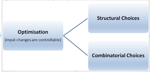
FIGURE 15.6 Structural and Combinatorial Optimisation
This topic is discussed briefly later in the chapter.
Uncertainty
The discussion so far has presented optimisation as the issue as to how to choose some input values whilst others are fixed. However, in some cases, these other variables may be subject to uncertainty. For example:
- One may try to find the optimum route to drive through a large town, either under the assumption that the transit time for each possible section of the route and the traffic lights and traffic conditions are known, or under the assumption that these items are uncertain. It is conceivable that the optimum route is the same, irrespective of whether uncertainty is considered. However, uncertainty can also impact risk-tolerances, so that if one needed to be sure to arrive at one's destination by a fixed time (such as to fix the time for a meeting), one may decide to choose a route that is longer on average but is less uncertain, so that a more reliable plan can be made.
- In the traditional frameworks used to describe the optimisation of financial portfolios, one is trying to choose the weights of each asset in the context in which the returns of each asset are uncertain (but with known values of the parameters that described the uncertainty, such as the mean and standard deviation of returns).
Integrated Approaches to Optimisation
From the above discussion, it is clear that in general one may have to reflect not only structural optimisation, but also (either or both of) combinatorial optimisation and uncertainty. For example:
- Faced with the structural decision as to whether either to stay at home or to meet a friend at the other side of town: if one chooses to meet the friend, there may be many possible combinations of routes that one could drive. At the same time, the length of time required to navigate each section of the route may be uncertain.
- When designing any large potential project (including when conducting risk assessment and risk management on it), one will generally have several options as to the overall structural design or technical solution. Within each, there will be design-related items that are to be optimised, as well as risks to mitigate, and residual risks or uncertainties that cannot be effectively mitigated further. Thus, the optimal project design and risk mitigation (or response) strategy will typically have elements both of structural and combinatorial optimisation, as well as uncertainty: structural optimisation about which context in which to operate (or overall technical solution to choose), combinatorial optimisation to find the best set of risk mitigation measures within that context and residual uncertainty that cannot be further reduced in an economically efficient way.
- Faced with the decision as to whether to proceed or not with a project, there may be characteristics which allow its scope to be modified after some initial information about its likely future success has been gained. For example, once initial information about a potential oil drilling (or pharmaceutical) project becomes available, the activities could be conducted as originally expected, or abandoned or expanded. Note that, although valuable, the information obtained may be imperfect, incur a cost to obtain it, and the process of doing so could delay the project (compared to deciding whether to proceed without this information). Real-life business situations in which a decision is possible either before or after uncertainty has been resolved (decision–chance–decision structures) are often termed “real options” situations.
Modelling Issues and Tools
Some important modelling issues that arise in optimisation contexts include:
- To ensure a clear and correct distinction between controllable and non-controllable inputs.
- To capture the nature of the optimisation within the model's logic. Where the optimisation is driven mainly by constraints, this is usually straightforward. Where it is driven by the U-shaped nature (in real life) of an output as an input varies, the model must also capture this logic. For example, a model which calculates sales revenues by multiplying price with volume may be sufficient for some simple sensitivity analysis purposes, but would be meaningless if used to find the optimal price, unless volume is made to depend on price (with higher prices leading to lower volumes). Thus, models which are intended to be used for optimisation purposes may have more demanding requirements on their logic than those that are to be used for simple “what-if” analysis, or if scenario approaches are used.
- To formulate the optimisation so that it has only one objective. Most optimisation algorithms allow for only one objective, whereas most business situations involve multiple objectives (and stakeholders with their own objectives). Thus, one typically needs to reformulate all but one of these as constraints. Whilst in theory the optimal solution would be the same in each, in practice, participants could often be (or feel themselves to be) at an advantage if their own objective is the one used for the optimisation (and at a disadvantage if their objective is instead translated into one of many constraints): psychologically, an objective has positive overtones, and is something that one should strive to achieve, whereas constraints are more likely to be de-emphasised, ignored or regarded as inconvenient items that can be modified or negotiated. Thus, when one's objective becomes expressed as only one item within a set of constraints, a focus on it is likely to be lost.
- Not to overly constrain the situation. A direct translation of management's objectives (when translated into constraints) often leads to a set of demands that are impossible to meet; so that optimisation algorithms will then not find a solution. Often, it can be useful to start with less constraints, so that an optimum can be found, and then seeks to show how the application of additional constraints changes the nature of the optimum solution, or leads eventually to no solution.
There is a large range of approaches and associated numerical techniques that may be applicable depending on the situation, including:
- Core tools for combinatorial optimisation, such as Excel's Solver. Where the optimisation problem is “multi-peaked” (or has certain other complex characteristics), Solver may not be able to find a solution, and other tools or add-ins (such as Palisade's Evolver based on genetic algorithms) may have a role.
- Combining optimisation with analytic methods. For example, in traditional approaches to the optimisation of financial portfolios, matrix algebra is used to determine the volatility of a portfolio based on its components. Thus, uncertainty has been “eliminated” from the model, so that standard combinatorial optimisation algorithms can be used.
- Combining optimisation with simulation. Where uncertainty cannot be dealt with by analytic or other means, one may have to use simulation. For example, with reference to the example earlier in the chapter, if there is uncertainty in the level of the cash flows for each project after its launch, then for every possible set of dates tried as a solution of the optimisation, a simulation would need to be run to see the uncertainty profile within that situation, with the optimum solution dependent on this (e.g. one may define the optimum one as the which maximises the average of the NPV, or alternatively as the one in which the NPV is above some figure with 90% frequency etc.). Where a full simulation is required for each trial of a potential optimal solution, it is often worth considering whether the presence of the uncertainty would change the actual optimum solution in any significant way. The potential time involved in running many simulations can be significant, whereas it may not generate any significantly different solutions. For example, in practice, the optimal route to travel across a large city may (in many cases) be the same irrespective of whether one considers the travel time for each potential segment of the journey to be uncertain or fixed. The implementation of such approaches may be done with several possible tools:
- Using VBA macros to automate the running of Solver and the simulation.
- Using Excel add-ins. For example, the RiskOptimizer tool that is in the Industrial version of the Excel add-in @RISK allows for a simulation to be run within each optimisation trial.
- Use of decision trees and lattice methods. Decision trees are often used due to their visual nature. In fact, decision trees can have a powerful numerical role that is independent of the visual aspect. When there is a sequential decision structure (in which one decision is taken after another, possibly within uncertain events in between), the optimum behaviour today can only be established by considering the future consequence of each possible choice. Thus, tree-based methods often use backward calculation paths, in which each future scenario must first be evaluated first, before a final view on today's decision can be taken. (The same underlying logic of backward calculations can in fact be implemented in Excel.) Generalisations of decision-tree approaches include those which are based on lattice methods, such as the finite difference or finite element methods that are applied on grids of data points; these are beyond the scope of this text.
- Decision trees may also need to be combined with simulation or other methods. For example, if there are uncertain outcomes that occur in between decision points, then each decision may be based on maximising the average (or some other property) of the future values. A backward process may need to be implemented to evaluate the last decision (based on its uncertain future outcomes), and once the choice for this decision is known, the prior decision can be evaluated; such stochastic optimisation situations are beyond the scope of this text.
Despite this complexity, one nice feature of many optimisation situations (especially those defined by a U-shaped curves) is that there are often several scenarios or choices that provide similar (if slightly sub-optimal) outcomes, since (around the optimum) point any deviation has a limited effect on the value of the curve (which is flat at the optimum point). Thus, sub-optimal solutions are often sufficiently accurate for many practical cases, and this may partly explain why heuristic methods (based on intuition and judgement, rather than numerical algorithms) are often used.