
6
Utility of Joint Population Exposure–Response Modeling Approach to Assess Multiple Continuous and Categorical Endpoints in Immunology Drug Development
Chuanpu Hu and Honghui Zhou
Janssen Research and Development, LLC, Global Clinical Pharmacology, 1400 McKean Road, Spring House, PA, 19477, USA
6.1 Introduction
Exposure–response (E–R) modeling of clinical endpoints is important for drug development by facilitating informative dose regimen selection. A widely used class of E–R models includes the Types I–IV indirect response (IDR) models [1]. These models are most often used to describe continuous physiological endpoints and their presumed consistency with the mechanism of drug action lends confidence to the model predictions. However, clinical trial endpoints are often disease scores that are not physiological variables. For example, two types of commonly used efficacy endpoints in rheumatoid arthritis (RA) are the 28‐joint disease activity score using CRP (DAS28) and 20%, 50%, and 70% improvement in the American College of Rheumatology disease severity criteria (ACR20, ACR50, and ACR70) [2]. In psoriatic arthritis (PsA), the Psoriasis Area and Severity Index (PASI) score, ranged 0–72 with 0.1 increments, is used in addition to the ACR criteria (for arthritis component) to measure the severity of the psoriatic component of the disease. Applications of IDR models to categorical clinical endpoints have emerged in the last decade via the latent variable approach [3].
Clinical trials may measure multiple clinical endpoints, and the magnitude of correlation between the clinical endpoints indicates the similarity level between the disease components that the endpoints are designed to measure. Even modeling of the individual endpoints, correlations between the endpoints may still remain for the between‐subject and within‐subject random effects. This level of similarity between the endpoints can be accounted for via joint modeling. In principle, joint modeling improves overall estimation efficiency and enables the prediction of joint probability distribution of the endpoints. The latter is particularly important because it allows for assessing the proportion of subjects achieving desirable responses simultaneously in more than one endpoint. For example, DAS28 and the ACR criteria are strongly correlated as they both measure arthritis severity. While the psoriasis and arthritis components represent different aspects of PsA, PASI (psoriatic component), and ACR (arthritis component) criteria may still show mild correlation, potentially in part due to the fact that improvement in PASI may make patients feel better and thus report better ACR criteria components such as swollen joint counts. Conceptually, these correlations differ in nature: in RA, they occur at the structural level; in PsA, they occur at the individual response level. Joint modeling allows the clarification of these differences and optimal integration of information. It allows the structural and individual level of correlations to be modeled respectively as that for between‐subject variability (BSV), and residual correlations, i.e. the correlation between observed endpoints at each time point conditional on BSVs.
The latent variable IDR framework enables the joint modeling of multiple clinical endpoints. While accommodating the endpoint correlations for BSV is relatively straightforward, it also allows the modeling of residual correlations between continuous and categorical endpoints; ordinarily, a difficult task even just from conceptual point of view. Implementation in NONMEM [4], a widely used software for population‐based pharmacokinetic (PK) and E–R modeling, however, requires a re‐writing of bivariate normal distributions as a conditional normal distribution [5]. When correlations occur at the structural level, it is possible for the joint model to be more parsimonious and yet still be able to better describe the individual endpoints, compared with separately modeling the endpoints [6]. This is because the joint model may better describe one endpoint through better estimation of subject‐specific random effects using information from the other endpoint.
Section 6.2 describes the latent variable IDR framework for modeling ordered categorical endpoints. Application examples of accommodating correlations at individual response level or at the structural level are given in Sections 6.3 and 6.4, respectively.
6.2 Latent Variable Indirect Response Models
For convenience in the later sections, the latent variable IDR framework is presented in notation of ACR criteria below. Because ACR20, ACR50, and ACR70 indicate different levels of improvement in the same disease, they can be combined into one ordered categorical endpoint, called ACR, having four possible outcomes: ACR = 1, if achieving ACR70; ACR = 2, if achieving ACR50 but not ACR70; ACR = 3, if achieving ACR20 but not ACR50; and ACR = 4, if not achieving ACR20.
The latent variable approach presumes an underlying latent variable such that a different level of the endpoint takes effect when the latent variable crosses certain thresholds. For this purpose, let L(t) be the latent variable and αk, k = 1, 2, 3 be the thresholds such that
Model L(t) as
where M(t) is the model predictor, ɛACR is distributed with mean 0 and variance 1, and σACR is the error standard deviation. Assuming that ɛACR ∼ N(0, 1) follows the standard normal distribution, then

In this setting of latent variables, σACR is not identifiable and may be assumed to be equal to 1, this gives
which corresponds to probit regression. Assuming ɛ follows a logistic distribution leads to logit regression. This insight leads to the following link between probit regression and logit regression. Since the variances for the standard logistic and the standard normal distributions are π2/3 and 1, respectively, scale‐related estimates, such as intercept and slope, from logistic regression could be expected to be larger than from probit regression by approximately a factor of 1.8 (≅![]() ) [6]. While logit regression may be more commonly used for single endpoint modeling, probit regression allows convenient joint modeling, as will be shown in the next section.
) [6]. While logit regression may be more commonly used for single endpoint modeling, probit regression allows convenient joint modeling, as will be shown in the next section.
The latent variable representation in Eq. (6.2) allows mechanism‐based models to be used for M(t). BSV is typically modeled at the intercept level with an additive normal distribution η ∼ N(0, ω2). Splitting the term −M(t) as placebo and drug effects, this leads to the mixed‐effect probit regression, as follows:
To stabilize parameter estimation, αk are reparameterized as (α2, d1, d3) with d1, d3 > 0 such that α1 = α2 − d1 and α3 = α2 + d3. The placebo effect may typically be modeled empirically, e.g. with an exponential function:
The drug effect is assumed to be driven by a latent variable RACR(t), which can be modeled by, e.g. in the case of a Type I IDR model:
where Cp is drug concentration, and kin,ACR, IC50,ACR, and kout,ACR are parameters in a Type I IDR model. It was further assumed that at baseline RACR(0) = 1, yielding kin,ACR = kout,ACR. The reduction of RACR(t) was assumed to drive the drug effect through:
where DEACR is a parameter to be estimated that determines the magnitude of drug effect.
Theoretically, the representation of drug effect in Eqs. (6.3)–(6.6) is equivalent to that of a change‐from‐baseline [7], and DEACR may be interpreted as the baseline of the latent variable [3]. The change‐from‐baseline model has one fewer parameter than the regular IDR model. One way to conceptualize its necessity is to realize that the latent variable is determined up to a constant and, therefore, needs to be normalized [3,8].
6.3 Residual Correlation Modeling Between a Continuous and a Categorical Endpoint
The latent variable IDR model representation provides a framework to model the residual correlation between an ordered categorical endpoint and a continuous endpoint. This is achieved in essence by treating the correlation as that between the latent variable and the continuous endpoint, which can then be modeled conveniently with multivariate normal distributions.
For example, in the PsA context, let the continuous endpoint PASI be modeled as
where PASI(t) is the observed PASI score, ɛPASI ∼ N(0, σPASI2) represents the within‐subject variability, and x(t) is the predictor model, e.g. a standard Type I IDR model. Then the potential residual correlation between ACR and PASI responses can be modeled using a bivariate normal distribution of ɛ = (ɛACR, ɛPASI) with a correlation parameter ρ. This is implemented by first developing the joint probability distribution prob[ACR(tij) = k, PASI(tij) = x] at time tij for the jth observation of subject i, conditional on the BSV ηi. From a standard statistical theory, the bivariate normal distribution of two random variables (X, Z) is characterized by (μX, μZ, σX2, σZ2, ρ), indicating the means and variances of X and Z along with their correlation. Furthermore, the conditional distribution of Z given X follows a normal distribution, i.e. Z|X = x ∼ N(μZ + σZ/σX ρ(x − μX), (1 − ρ2) σZ2). Therefore, conditional on the BSV ηi and interpreting X as observed PASI scores, μX as x(t) in Eq. (6.7), Z as the ACR latent variable error σACR ɛACR in Eq. (6.1) and with μZ given by the right‐hand side of Eq. (6.2), and letting f be the probability density function of the standard normal distribution, then
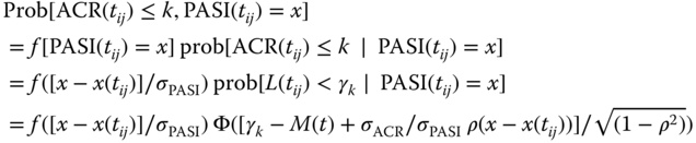
where the conditioning on ηi is implicitly present in all terms but omitted for the ease of notation. As noted above, Eq. (6.2), σACR = 1 may be chosen. Let rij = [x − x(tij)]/σPASI, the above becomes
Let yi,j = [ACR(tij), PASI(tij)] = (k, x) be the jth observation vector of length 2 of subject i. Eq. (6.8) allows the likelihood of yi,j conditional on ηi to be calculated as l(yi,j|ηi) = Prob[ACR(tij) ≤ k, PASI(tij) = x] − Prob[ACR(tij) ≤ (k − 1), PASI(tij) = x].This allows the correlation model to be implemented in standard software, e.g. NONMEM [4]. For sake of theoretical completeness, the marginal likelihood of subject i is given by ![]() , where θ represents the ACR–PASI model fixed‐effect parameters in Eqs. (6.3) and (6.7), and f(η) is the multivariate density function of the BSVs. The overall likelihood is the product of the marginal likelihood over all subjects.
, where θ represents the ACR–PASI model fixed‐effect parameters in Eqs. (6.3) and (6.7), and f(η) is the multivariate density function of the BSVs. The overall likelihood is the product of the marginal likelihood over all subjects.
6.3.1 Application Example: Ustekinumab in Psoriatic Arthritis (PsA)
An application example of PsA residual joint modeling of PASI and ACR criteria is described below, based on the data from PSUMMIT I [9], a phase III clinical trial in subjects with PsA subjects following subcutaneous (SC) administration of ustekinumab through the primary endpoint at Week 24. Ustekinumab (Stelara®; Janssen Biotech, Inc., Horsham, PA, USA) is a human immunoglobulin G1 monoclonal antibody that binds with high specificity and affinity to the shared p40 subunit of interleukin (IL)‐12 and IL‐23 and blocks interaction with the IL‐12Rβ1 CEll surface receptor and is approved for the treatment of plaque psoriasis, PsA, and Crohn's disease.
PSUMMIT I is a randomized, double‐blind, placebo‐controlled, parallel, multicenter three‐arm trial (with early escape at Week 16) in subjects who have active PsA despite current or previous therapy with disease‐modifying anti‐rheumatic drugs and/or nonsteroidal anti‐inflammatory drugs (NSAIDs) and were not previously exposed to anti‐tumor necrosis factor (TNF) agents. Approximately, 600 subjects were randomly assigned to treatment with SC injections of ustekinumab 45 and 90 mg, or placebo at Weeks 0 and 4 followed by every 12 weeks (q12w) dosing with the last dose administered at Week 88. As it is ethically undesirable to keep subjects on placebo extensively long, subjects randomized to placebo crossed over to receive ustekinumab 45 mg at Weeks 24 and 28 followed by q12w dosing with the last dose administered at Week 88. Data from the Week 24 database lock were used for this analysis. The efficacy measures that were modeled included ACR20, ACR50, and ACR70 responses and PASI scores. PK samples were scheduled to be collected at Weeks 4, 12, 16, 20, and 24, and ACR20, ACR50, and ACR70 responses were scheduled to be collected at Weeks 4, 8, 12, 16, 20, and 24. In addition, predose PK samples were also collected at Week 0 and PASI scores were measured at Weeks 0, 12, 16, and 24. Table 6.1 shows the number of subjects and observations by treatment groups.
Table 6.1 Number of subjects and observations in study PSUMMIT I.
| Treatment | Number of subjects | Number of PK observations | Number of ACR observations | Number of PASI observations |
| Placebo | 205 | 111 | 1146 | 768 |
| 45 mg | 205 | 871 | 1199 | 797 |
| 90 mg | 204 | 928 | 1148 | 768 |
| Total | 614 | 1910 | 3493 | 2333 |
PK, pharmacokinetic; ACR, American College of Rheumatology disease severity criteria; and PASI, Psoriasis Area Severity Index.
6.3.1.1 Population PK Modeling of Ustekinumab in PsA
To facilitate E–R modeling, a confirmatory population PK analysis approach [10,11] using a one‐compartment model with first‐order absorption was planned and implemented. Based on a previous study by Zhu et al. [12], a one‐compartment model with first‐order absorption was prespecified. Baseline body weight and presence of immune response were the only clinically relevant covariates, as expected, which were included in the final reduced model. The results were consistent with earlier analyses from the psoriatic patient population [11,12].
6.3.1.2 E–R Modeling of Ustekinumab in PsA
The population PK parameters and data (PPP&D) approach described by Zhang et al. [13] was used for the E–R model estimation by fixing the population PK model parameters estimates and retaining the ustekinumab concentrations in the dataset to allow individual PK profiles to be determined. Parameter estimation was implemented in NONMEM using the Laplace option. Model selection was based on the NONMEM objective function values (OFVs), which are approximately – two times log likelihood. A change in OFV of 7.88 corresponds to a nominal p‐value of 0.005 and was judged as significant evidence to include an additional parameter.
Placebo effect modeling for PASI scores was initially attempted but could not be supported by the data. Consequently, the PASI scores were modeled using a basic Type I IDR model, with the predictor x(t) governed by
The BSV on baseline b = kin,PASI/kout,PASI, called ηb, was modeled with lognormal distribution in the form bi = b exp·(ηb,i), where i indicates the ith subject and ![]() . BSV on other parameters were explored but could not be supported by the data.
. BSV on other parameters were explored but could not be supported by the data.
The joint residual modeling approach was applied by fitting Eqs. (6.3)–(6.9) to PASI and ACR data. Parameter estimates are given in Table 6.2.
Table 6.2 Initial PASI‐ACR exposure–response model parameter estimates.
| α2 | d1 | d3 | rp,ACR (d − 1) | IC50,ACR (μg ml − 1) | kout,ACR (d−1) | DEACR | Var(η) | |
| ACR parameter estimate (% RSE) | −2.13 (9.5) | 1.1 (5.7) | 1.26 (3.9) | 0.0157 (32.2) | 2.5 (38.9) | 0.00423 (108.3) | 4.18 (74.6) | 1.85 (9.6) |
| b | IC50,PASI (μg ml − 1) | kout,PASI (d−1) | Var(ηb) | σPASI | ρa | |||
| PASI parameter estimate (% RSE) | 4.87 (5.4) | 0.099 (46.2) | 0.0145 (11.1) | 1.02 (6.1) | 2.98 (6.1) | 0.173 (28.2) |
ACR, American College of Rheumatology disease severity criteria; PASI, Psoriasis Area Severity Index; RSE, relative standard error; α2, d1, d3, intercept parameters; rp,ACR, rate of placebo effect onset for ACR; IC50,ACR, potency for ACR; kout,ACR, disease amelioration rate for ACR; DEACR, drug effect for ACR; Var(η), variance of between‐subject variability for ACR; b, baseline; IC50,PASI, potency for PASI; kout,PASI, disease amelioration rate for PASI; Var(ηb), variance of between‐subject variability for PASI; σPASI, standard deviation of within‐subject variability for PASI; ρ, residual correlation between ACR and PASI score.
aShared between ACR and PASI models.
Estimation precision of baseline parameters was generally reasonable, with relative standard error (RSE) ranging from 3.9% to 9.5%. Drug effect parameter estimation was mostly relatively imprecise with RSE ranging from 11.1% to 108.3%, due to pharmacodynamic (PD) evaluations at only a few time points. Disease effect parameter estimates were quite different between ACR and PASI scores, indicating differences in disease characteristics and drug action. Introducing a correlation between the BSV terms (η for ACR and ηb for PASI) did not result in any meaningful improvement of the fit (NONMEM objective function change <1), suggesting the lack of correlation among the two disease components. The residual‐correlation term ρ was deemed significant, with NONMEM objective function change >13. The magnitude (0.173) was however mild. These results suggested a weak correlation between the ACR and PASI assessments.
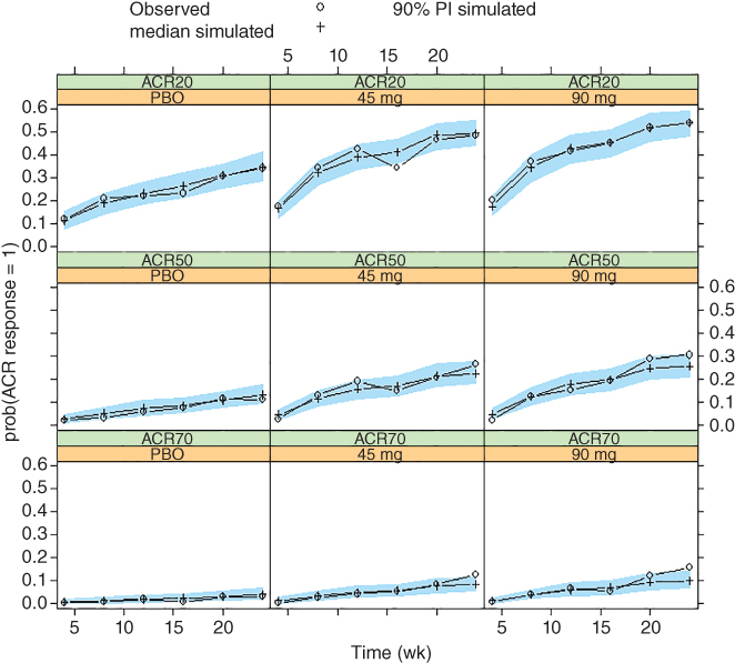
Figure 6.1 Visual predictive check of American College Rheumatology (ACR) response frequencies for PSUMMIT I data. Median model predictions at planned observation times and 90% prediction intervals (PIs) are overlaid with observed ACR response frequencies by treatment. ACR20/50/70, 20%/50%/70% improvement in the American College of Rheumatology criteria; PBO, placebo.
Visual predictive checks (VPCs) [14] were also performed by simulating 500 replicates of the dataset and comparing simulated and model‐predicted responses. In general, it is desirable to evaluate the joint distribution of the endpoints when modeling of multiple endpoints. In this scenario, however, due to the lack of correlation of BSVs and the mild residual correlation, separate VPCs for ACR and PASI scores were expected to suffice. Results for the ACR model are shown in Figure 6.1. The 90% predicted intervals (PIs) of the simulated ACR response frequencies at planned assessment visits are shown in overlay with the observed ACR response frequencies, grouped by treatment. Minor discrepancies were present, likely due to data variability. Overall, the model described observed data reasonably well.
VPCs results for PASI scores are shown in Figure 6.2. The decrease of observed and predicted scores for placebo at Week 24 was due to the fact that these subjects crossed over to active treatment earlier than planned. This time point was included in the placebo group for convenience reasons, even though it does not reflect the placebo response. The difference between observed and predicted scores for the 45 mg group may be attributed to baseline differences. The difference, in principle, should not affect prediction of PASI improvement from baseline. Overall, the model described the data well.
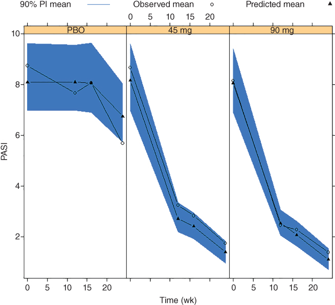
Figure 6.2 Visual predictive check of Psoriasis Area and Severity Index (PASI) scores for PSUMMIT I data. Mean model predictions at planned observation times and 90% prediction intervals (PIs) are overlaid with observed PASI scores by treatment. PBO, placebo.
The joint model was further validated with external data of an additional study, PSUMMIT II, similarly designed as PSUMMIT I but with approximately 300 subjects, half of which were TNF‐experienced. More details may be found in Hu et al. [5].
6.3.1.3 Application Example Summary of Ustekinumab in PsA
A general framework has been built for joint E–R modeling of continuous (PASI) and categorical (ACR) clinical endpoints. This modeling framework allows for the accounting of the correlation of BSV as well as residual correlations between the endpoints. This approach generally achieves increased analysis efficiency and, more importantly, allows better prediction of the joint distribution of the endpoint outcome, e.g. the proportion of subjects achieving sufficient improvement in both disease components of PsA as measured by ACR20 and PASI75. A conditional approach allowing the estimation of residual correlation to be implementable in NONMEM is provided. This method can be easily applied to situations involving multiple continuous endpoints. It also extends to the situation when the categorical endpoint is of the nature of bounded outcome scores [15,16]. For PsA, the weak but positive residual‐correlation between the ACR and PASI scores was informative and consistent with clinical expectations.
6.4 Structural Correlation Modeling Between a Continuous Endpoint and a Categorical Endpoint
The latent variable IDR model representation allows similarities of model parameters between an ordered categorical endpoint and a continuous endpoint to be explored, which includes fixed‐effect parameters as well as BSVs. More importantly, when the endpoints measure similar disease components, the framework allows the possibility of having the continuous endpoint function as the latent variable for the ordered categorical variable. This can allow additional BSVs to be used in describing the categorical endpoint, using information in the continuous endpoint. In this regard, joint modeling can achieve much parsimony than ordinarily expected, as shown in the application example below.
6.4.1 Application Example: Rheumatoid Arthritis
DAS28 and ACR criteria response were available in data from two phase III, parallel, placebo‐controlled clinical trials of intravenously administered mAb X, Study 1 [17] and Study 2 [18], in patients with active RA despite prior use of methotrexate (MTX) therapy. Data used were the same as in the E–R modeling of ACR20, ACR50, and ACR70 response described previously [7], with the additional inclusion of DAS28 scores. Briefly, Study 1 investigated the mAb X dose regimen of 2 mg kg−1 given at Weeks 0, 4, and every eight weeks thereafter, briefly written hereafter as the q8 weekly regimen. Study 2 studied the mAb X dose regimens of 2 and 4 mg kg−1 given every 12 weeks. Both trials had MTX as placebo control arms, and subjects on the placebo arms were switched to the active arms of mAb X + MTX at Week 16, at which time they were eligible for early escape to receiving rescue medications. The numbers of subjects in the E–R modeling dataset were 395, 197, 129, 126, and 129, respectively, for the following treatment arms: mAb X 2 mg kg−1 + MTX q8 weeks (Study 1), placebo 1 (MTX, Study 1), mAb X 2 mg kg−1 + MTX q12 weeks (Study 2), mAb X 4 mg kg−1 + MTX q12 weeks (Study 2), and placebo 2 (MTX, Study 2).
6.4.1.1 Population PK Modeling of mAb X in Rheumatoid Arthritis
A population PK analysis using a two‐compartment linear model implemented in NONMEM was performed using data from patients available for E–R modeling and additional data from other studies. The model described the data adequately and the details of the PK study data and analysis are described elsewhere. Results were consistent with a previous confirmatory population PK analysis [11]. Empirical Bayesian parameter estimates were then used in a sequential modeling approach for the E–R modeling discussed below.
6.4.1.2 E–R Modeling of mAb X in Rheumatoid Arthritis
Parameter estimation was implemented in NONMEM using the Laplace option for early exploration and the Importance Sampling (IMP) method for key model runs. Model selection was based on the NONMEM OFVs. A change in NONMEM OFV of 10.83, corresponding to a nominal p‐value of 0.001, was used as a criterion of including an additional parameter. VPC was used for model evaluation by simulating 500 replicates of the dataset and comparing simulated and model‐predicted DAS28 score and ACR response frequencies over the treatment period.
DAS28 Model Component
DAS28 scores were modeled with an IDR‐based model applied in earlier E–R analyses [19] as
where DAS28(t) is the observed DAS28 score at time t, b is baseline DAS28 score, fDAS28,p(t) is placebo effect, fDAS28,d(t) is drug effect, and ɛ ∼ N(0, σ2) represents the within‐subject variability. The placebo effect was modeled empirically as
where 0 ≤ Fp,DAS28 ≤ 1 is the fraction of maximum placebo effect and rDAS28 is the rate of onset. The drug effect was modeled with
where 0 ≤ Emax ≤ 1 represents fraction of maximum drug effect and, following a previous approach [15,19], the drug effect was assumed to be driven by a latent variable RDAS28(t) governed by
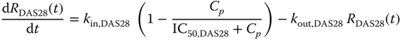
It was further assumed that at baseline RDAS28(0) = 1, yielding kin,DAS28 = kout,DAS28.
Equations (6.10)–(6.13) and (6.3)–(6.6) were first fitted to DAS28 and ACR data separately and then simultaneously with shared parameters explored.
Initial DAS28 Model of mAb X in Rheumatoid Arthritis
Figure 6.3 shows the observed DAS28 time course by treatment group. High variability was apparent, both between and within subjects. In addition, baseline DAS28 in Study 1 appeared to be notably larger than that in Study 2. Therefore, an additional parameter bs was used to account for the baseline difference between Study 1 and Study 2.
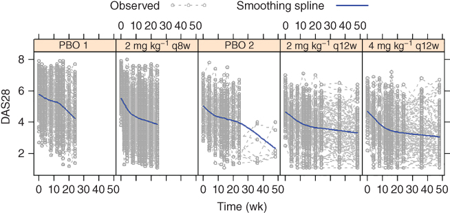
Figure 6.3 A random sample of observed 28‐joint disease activity (DAS28) scores with 30 subjects in each treatment group overlaid with smoothing spline.
Further modeling explorations using the Laplace option could not reliably estimate any more BSV terms than those on b and IC50, and led to a sizable estimate (≅5, or >70%) for BSV on IC50. While parameter estimate appeared reasonable, standard error (SE) estimation appeared unstable. Since the adequacy of the Laplace approximation degrades as the magnitude of BSV increases, the IMP estimation option in NONMEM was used for key model runs. BSV terms were included on b, pDAS28, IC50,DAS28, and Emax, with a full variance–covariance matrix accounting for their correlations. Attempting to reduce the BSV terms or the correlation parameters or to include additional BSV terms resulted in either notably worsening or lack of sufficient improvement in the fit. Table 6.3 shows the parameter estimates. Estimation precision was reasonable, with SEs generally an order of magnitude lower than the estimates. SE is presented in order to provide appropriate comparison of estimation precision among different models. Figure 6.4 shows the VPC results, where high variability of the observed data is apparent which is consistent with what is observed in Figure 6.3. Overall, the model reasonably described the observed data trends.
Table 6.3 DAS28 exposure–response model main effect parameter estimates.
| Fixed and residual effect estimate (SE) | b | pDAS28 | IC50,DAS28 (μg ml − 1) | Emax | rDAS28 (d−1) | kout,DAS28 (d−1) | bs | ρa | σDAS28 |
| Initial separate model | 4.91 (0.0436) | 0.161 (0.0104) | 0.132 (0.0681) | 0.23 (0.0145) | 9.54 × 10⁻³ (7.46 × 10⁻⁴) | 0.16 (0.03) | 0.961 (0.0578) | NA | 0.632 (5.75 × 10⁻³) |
| Final joint model | 4.93 (0.0428) | 0.15 (9.72 × 10⁻³) | 1.24 (0.0742) | 0.221 (0.0296) |
1.01 × 10⁻² (7.89 × 10⁻⁴) |
0.125 (0.0154) | 0.932 (0.0566) | −0.655 (0.0103) | 0.624 (5.48 × 10⁻³) |
Initial ACR Model of mAb X in Rheumatoid Arthritis
Equations (6.3)–(6.6) were fitted to the ACR response data. Table 6.5 shows the parameter estimates.
Estimation precision was reasonable. IC50 and kout estimates were similar to those obtained previously [7]. From a theoretical perspective, drug effect (DE) estimate from logistic regression could be expected to be larger than that from probit regression by approximately a factor of 1.8, as mentioned in Section 6.3. Taking account of this difference, differences between the DE estimates did not appear to be unexpected. Other parameter estimates were different in part due to the earlier use of a reduced placebo model. Estimation precision was reasonable, with SEs at generally a magnitude lower than the estimates. VPC results are shown in Figure 6.5, which are similar to those in the previous analyses [7] as could be expected [3]. As previously noted, the high observed placebo responses at Weeks 20 and 24 may be due to the early escape of some patients [7].
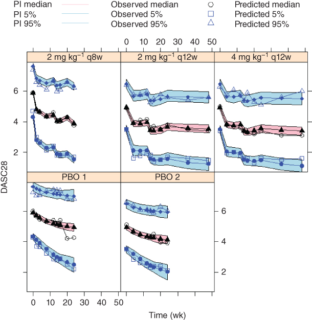
Figure 6.4 Visual predictive check of the 28‐joint disease activity (DAS28) score for the initial model. The 5th, 50th, and 95th percentiles of observed DAS28 scores are overlaid with the 90% prediction intervals (PI) of their model predictions at planned observation times by treatment. PBO, placebo. (See insert for color representation of this figure.)
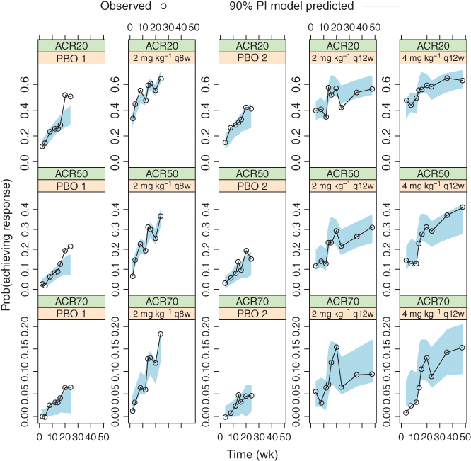
Figure 6.5 Median model predictions at planned observation times and 90% prediction intervals (PI), in overlay with observed American College Rheumatology (ACR) response frequencies, for the initial ACR model. ACR20/50/70, 20%/50%/70% improvement in the American College of Rheumatology criteria.
Joint DASC28‐ACR E–R Model of mAb X in Rheumatoid Arthritis
The base scenario of fitting Eqs. (6.3)–(6.6) and (6.10)–(6.13) simultaneously with no shared parameters between the DAS28 and ACR model components is equivalent to fitting the DAS28 and ACR models separately. Consistent with this, the sum of the OFVs of the DAS model and ACR models was nearly identical to the OFV of the simultaneously fitted model with no shared parameters. Tables 6.3 and 6.4 show that the rate parameters, namely rDAS28 and kout, appeared similar between the endpoints, along with IC50. Indeed, this was substantiated by the joint model evaluations showing insignificant OFV change for sharing each parameter in the joint model.
Table 6.4 DAS28 exposure–response model between‐subject random effect parameter estimates.
| Variance–covariance matrix of between‐subject random effect estimate (SE) | |||||
| Initial separate model | b | pDAS28 | IC50,DAS28 | Emax | |
| b | 0.0177 (1.26 × 10⁻³) | ||||
| pDAS28 | 0.0386 (9.84 × 10⁻³) | 1.95 (0.203) | |||
| IC50,DAS28 | 0.0605 (0.0294) | −0.838 (0.564) | 1.6 (0.652) | ||
| Emax | −0.0506 (0.0114) | 0.173 (0.156) | −0.0596 (0.354) | 0.91 (0.117) | |
| Final joint model | B | pDAS28 | IC50,DAS28 | Emax | |
| b | 0.0201 (1.24 × 10⁻³) | ||||
| pDAS28 | 0.0248 (0.0101) | 2.03 (0.241) | |||
| IC50,DAS28 | 0.0887 (0.0403) | −0.89 (1.15) | 3.29 (2.25) | ||
| Emax | −0.0197 (0.0102) | 0.101 (0.148) | 0.193 (0.531) | 1.12 (0.237) | |
This result motivated the question of whether further similarities between the endpoints could be found. It could be hypothesized that, based on binding, a single latent variable could govern both endpoints through IDR models. The similarity of the kout parameters suggested the possibility of using a single IDR model instead of two. The question however is in what sense the placebo and drug effect could be considered similar for both endpoints, particularly because DAS28 and ACR endpoints have different scales. This rationale motivated the use of DAS28 change‐from‐baseline, since the latent variable corresponding to ACR endpoints is defined only up to a constant. Following the motivation given in Section 6.3, this led to the following ACR model in place of Eq. (6.3)–(6.6):
where M(t) = Lm[fDAS28,p(t) + fDAS28,d(t)]/b is the scaled change‐from‐baseline DAS28 score model prediction given in Eq. (6.10), with BSV terms as given in the initial DAS28 score model.
Fitting Eqs. (6.10)–(6.14) simultaneously to the DAS28 and ACR response data resulted in a NONMEM objective function decrease of over 2000, indicating a significant improvement of the fit, despite using four fewer parameters than the base scenario. Inclusion of the residual correlation between DAS28 and ACR responses further reduced the NONMEM objective function by over 1900. This model was considered as the final one, with parameter estimates of the DAS28 and ACR response components given in Tables 6.3–6.5, respectively.
Table 6.5 ACR exposure–response model parameter estimates.
| Parameter estimate (SE) | α2 | d1 | d3 | rp,ACR (d−1) | kout (d−1) | IC50 (μg ml − 1) | DEACR | Fp,ACR | Lm | ω2 |
| Initial separate model | −1.47 (0.121) | 1.06 (0.0321) | 1.29 (0.0266) | 0.00916 (1.17 × 10⁻³) | 0.111 (0.0209) | 0.168 (0.043) | 1.43 (0.0948) | 1.93 (0.0961) | NA | 1.69 (0.111) |
| Final joint model | −4.69 (0.0826) | 1.21 (0.0356) | 1.43 (0.0297) | NA | NA | NA | NA | NA | 0.125 (2.79 × 10⁻³) | 0.38 (0.0397) |
ACR, American College of Rheumatology disease severity index; DAS28, 28‐joint disease activity score; SE, standard error; α2, d1, d3, intercepts parameters; rp,ACR, rate of placebo effect onset; kout,ACR, disease amelioration rate; IC50,ACR, potency; DEACR, drug effect; Fp,ACR, fraction of maximum placebo effect onset; Lm, maximum latent variable effect; ω2, variance of between‐subject variability; NA, not applicable.
Tables 6.3 and 6.4 show that for DAS28, the joint model parameter estimates and associated SEs were generally similar to those obtained with the initial model using only DAS28 data. Table 6.5 shows that for ACR component, the joint model used no additional parameters for the placebo and drug effects other than the scaling parameter Lm. Estimates of the intercept parameter α2 between the initial and joint models are not directly comparable, as the average intercept value is determined up to a constant with the latent variable [3]. Estimates of d1 and d3, the intercept differences, were similar between the initial and joint models. The estimate of ω2 was smaller in the joint model, due to the fact that the treatment effect predictor M(t) in Eq. (6.14) contains BSV components, whereas Eqs. (6.3)–(6.6) do not. This contribution of BSV components of the DAS28 model is the main cause for the improved fit of the joint model. Coupled with a high absolute value of correlation parameter estimate (0.655) shown in Table 6.3, this confirms that the two endpoints measure largely the same component of the disease.
VPC results of the joint model for DAS28 was visually indistinguishable as shown in Figure 6.4, and thus is not shown. This is consistent with the similarity between the parameter estimates of the joint and the separate models. VPC results of the joint model for the ACR response are shown in Figure 6.6. It is noted that the VPC results of the joint model before incorporating the residual correlation component were visually indistinguishable from Figure 6.4 and are not shown. The results appeared largely similar to those in Figure 6.5; where differences occurred, it may appear difficult to determine whether the joint model or the individual ACR model prediction better represent reality.
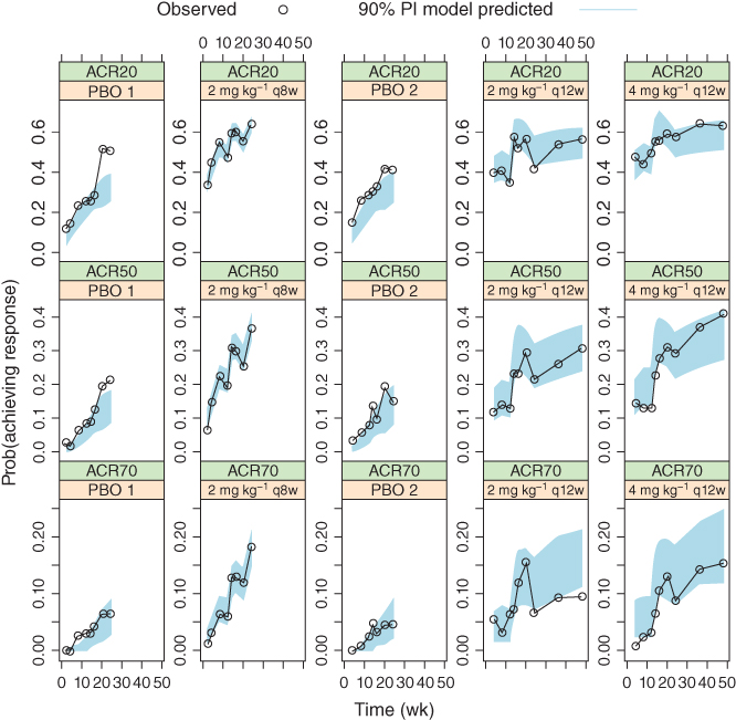
Figure 6.6 Median model predictions at planned observation times and 90% prediction intervals (PI), in overlay with observed American College Rheumatology (ACR) response frequencies, for the final joint model. ACR20/50/70, 20%/50%/70% improvement in the American College of Rheumatology criteria.
However, it is reasonable to expect that the ACR70 response rates for the placebo arms to be small in early treatment periods, and the joint model prediction in Figure 6.6 is better than the ACR model prediction in Figure 6.5. This may be attributed to the more reasonable partitioning of BSV onto additional model parameters under the joint model rather than only at the intercept level under the ACR model. It can be seen that under Eq. (6.14), the expected ACR response rate at time of (or near) 0 is given by [3,20]
and that the larger predicted ACR70 response rate in the separate model was caused by the larger ω2 estimate. In contrast, the joint model had part of this BSV component partitioned onto other parameters, namely through BSV terms on b, pDAS28, IC50,DAS28, and Emax, none from which contributed to the BSV of ACR responses at time near 0 since M(0) = 0, which led to the smaller overall BSV predictions near time 0. This, therefore, suggested that the latent variable joint model may partition the BSV more appropriately by allowing it to vary over time, as opposed to remaining constant under the separate model.
In order to understand the source of improvement in the joint model fitting, it may be tempting to examine the OFV changes in the DAS component and ACR component. However, this would be exceedingly difficult because the two components are not independent without conditioning on the BSV terms. Nevertheless, there are two relevant observations in comparing the separate and the joint models: (i) in the DAS component, changes of parameter estimates and associated SE were minor, and the VPC results were virtually unchanged; (ii) in the ACR component, the original BSV variance ω2 was markedly reduced in the joint model. These suggested that the improvement in OFV mostly came from the ACR component, through the presence of the additional BSV terms in the latent variable.
6.4.1.3 Application Example Summary
This analysis supported and utilized the relatedness between DAS28 and ACR responses that are designed to measure the same disease component through shared structural model component along with the related BSVs and the residual correlation. A common view on the modeling of multiple endpoint is that, while joint modeling may improve the overall fit as measured by the likelihood or predictions of correlated responses, it would not affect the descriptions or predictions of the individual endpoints [21]. On the other hand, the joint model for DAS28 and ACR responses developed here improved the characterization of the ACR response, in a manner unrelated to the residual correlation component. This is due to the fact that the number of random effects used to describe ACR response actually increased by three under the joint model, namely through the BSV terms under the latent variable M(t) in Eq. (6.14). The estimation of these additional random effects could not be reliably supported by ACR data alone [7] and was made possible only with the added DAS28 data under the joint model framework. This feature may hold true more generally when the endpoints include both the continuous and the categorical types, where the continuous endpoint data may support random effects not estimable from the categorical endpoint data alone, and thus resulting in better description of the categorical endpoints. This demonstrates more clearly the improvement achievable by the joint modeling approach than the previous applications [5,21]. It is noted that the joint approach requires considerably more effort and computational time. On the other hand, categorical endpoint modeling alone typically cannot support the estimation of more than one BSV term. It is noted that the magnitude of BSV at the intercept level determines the response probability together with underlying exposure, as can be seen in Eq. (6.15) (see more details in Ref. [20]). The question thus arises on how this would affect model predictions, especially the associated variability. The joint model can provide valuable insights into this important question in clinical development.
In this example, a study effect term was used to account for baseline DAS28 differences between the two studies. Estimation results of the remaining parameters were similar to those in an earlier model without the study effect on baseline. However, the VPC of this earlier model showed systematic differences between the model predicted and observed data trends, which could easily lead to doubt on the predictive ability of the model. The study effect has descriptive but not predictive value, and the inclusion of such covariates should be exercised with caution. As subjects are randomized only within the studies and not to them, the study effect on baseline served the purpose of adjusting for imbalances between studies. Inclusion of study effect on other model components could easily lead to interpretation difficulties and is thus generally not advisable.
6.5 Conclusion
Joint E–R modeling of multiple, continuous, and categorical clinical endpoints can be effectively achieved through the latent variable IDR framework. This can provide unique advantages in insightful explanation of the nature of associations, as well as substantial gains in integrating information among the endpoints. As illustrated by the examples in this chapter, in the case that the endpoints describe different disease components, joint modeling can confirm the source of mild correlations, and in the case that endpoints describe similar disease components, better description of an ordered categorical endpoint can be achieved by leveraging information from a continuous endpoint. Even though the presented examples are in rheumatoid arthritis and PsA, the same or similar joint E–R modeling approach can find it utility in other immune‐mediated inflammatory diseases such as psoriasis or inflammatory bowel diseases (Crohn's disease, ulcerative colitis).
References
- 1 Sharma, A. and Jusko, W.J. (1996). Characterization of four basic models of indirect pharmacodynamic responses. J. Pharmacokinet. Biopharm. 24 (6): 611–635.
- 2 Felson, D.T., Anderson, J.J., Boers, M. et al. (1995). American College of Rheumatology. Preliminary definition of improvement in rheumatoid arthritis. Arthritis Rheum. 38 (6): 727–735.
- 3 Hu, C. (2014). Exposure–response modeling of clinical end points using latent variable indirect response models. CPT Pharmacometrics Syst. Pharmacol. 3: e117.
- 4 Beal, S.L., Sheiner, L.B., Boeckmann, A., and Bauer, R.J. (2009). NONMEM User's Guides (1989–2009). Ellicott City, MD: Icon Development Solutions.
- 5 Hu, C., Szapary, P.O., Mendelsohn, A.M., and Zhou, H. (2014). Latent variable indirect response joint modeling of a continuous and a categorical clinical endpoint. J. Pharmacokinet. Pharmacodyn. 41 (4): 335–349.
- 6 Hu, C. and Zhou, H. (2016). Improvement in latent variable indirect response joint modeling of a continuous and a categorical clinical endpoint in rheumatoid arthritis. J. Pharmacokinet. Pharmacodyn. 43 (1): 45–54.
- 7 Hu, C., Xu, Z., Mendelsohn, A., and Zhou, H. (2013). Latent variable indirect response modeling of categorical endpoints representing change from baseline. J. Pharmacokinet. Pharmacodyn. 40 (1): 81–91.
- 8 Hutmacher, M.M., Krishnaswami, S., and Kowalski, K.G. (2008). Exposure–response modeling using latent variables for the efficacy of a JAK3 inhibitor administered to rheumatoid arthritis patients. J. Pharmacokinet. Pharmacodyn. 35: 139–157.
- 9 McInnes, I.B., Kavanaugh, A., Gottlieb, A.B. et al. (2013). Efficacy and safety of ustekinumab in patients with active psoriatic arthritis: 1 year results of the phase 3, multicentre, double‐blind, placebo‐controlled PSUMMIT 1 trial. Lancet 382 (9894): 780–789.
- 10 Hu, C., Zhang, J., and Zhou, H. (2011). Confirmatory analysis for phase III population pharmacokinetics. Pharm. Stat. 10 (7): 812–822.
- 11 Hu, C. and Zhou, H. (2008). An improved approach for confirmatory phase III population pharmacokinetic analysis. J. Clin. Pharmacol. 48 (7): 812–822.
- 12 Zhu, Y., Hu, C., Lu, M. et al. (2009). Population pharmacokinetic modeling of ustekinumab, a human monoclonal antibody targeting IL‐12/23p40, in patients with moderate to severe plaque psoriasis. J. Clin. Pharmacol. 49 (2): 162–175.
- 13 Zhang, L., Beal, S.L., and Sheiner, L.B. (2003). Simultaneous vs. sequential analysis for population PK/PD data I: best‐case performance. J. Pharmacokinet. Pharmacodyn. 30 (6): 387–404.
- 14 Karlsson M.O. and Holford N.H.G. (2008). A Tutorial on Visual Predictive Checks 2008 [updated 2008]. www.page‐meeting.org/?abstract=1434 (accessed 05 October 2018).
- 15 Hu, C., Yeilding, N., Davis, H.M., and Zhou, H. (2011). Bounded outcome score modeling: application to treating psoriasis with ustekinumab. J. Pharmacokinet. Pharmacodyn. 38 (4): 497–517.
- 16 Hutmacher, M.M., French, J.L., Krishnaswami, S., and Menon, S. (2011). Estimating transformations for repeated measures modeling of continuous bounded outcome data. Stat. Med. 30 (9): 935–949.
- 17 Weinblatt, M.E., Bingham, C.O., Mendelsohn, A.M. et al. (2012). Intravenous golimumab is effective in patients with active rheumatoid arthritis despite methotrexate therapy with responses as early as week 2: results of the phase 3, randomised, multicentre, double‐blind, placebo‐controlled GO‐FURTHER trial. Ann. Rheum. Dis. 72 (3): 381–389.
- 18 Kremer, J., Ritchlin, C., Mendelsohn, A. et al. Golimumab, a new human anti‐TNFα antibody, administered intravenously in patients with active rheumatoid arthritis: 48‐week efficacy and safety results of a phase 3, randomized, double‐blind, placebo‐controlled study. Arthritis Rheum. 62 (4): 917–928.
- 19 Hu, C., Szapary, P.O., Yeilding, N., and Zhou, H. (2011). Informative dropout modeling of longitudinal ordered categorical data and model validation: application to exposure–response modeling of physician's global assessment score for ustekinumab in patients with psoriasis. J. Pharmacokinet. Pharmacodyn. 38 (2): 237–260.
- 20 Hutmacher, M.M. and French, J.L. (2011). Extending the latent variable model for extra correlated longitudinal dichotomous responses. J. Pharmacokinet. Pharmacodyn. 38: 833–859.
- 21 Laffont, C.M., Vandemeulebroecke, M., and Concordet, D. (2014). Multivariate analysis of longitudinal ordinal data with mixed effects models, with application to clinical outcomes in osteoarthritis. J. Am. Stat. Assoc. 109 (507): 955–966.