
18
Case Examples of Using Quantitative Pharmacology in Developing Therapeutic Proteins in Multiple Sclerosis – Peginterferon Beta‐1a, Daclizumab Beta, Natalizumab
Xiao Hu1,2Yaming Hang1,3Lei Diao1,4 Kumar K. Muralidharan1 and Ivan Nestorov1
1Biogen, 225 Binney Street, Cambridge, MA, 02142, USA
2Wave Life Sciences, 733 Concord Ave, Cambridge, MA, 02138, USA
3Takeda Pharmaceuticals International Co., Cambridge, MA, 02138, USA
4BMS China, 15F, Wheelock Square, 1717 West Nanjing Road, Shanghai, China
18.1 Introduction
Multiple sclerosis (MS) is an autoimmune inflammatory disorder of central nervous system (CNS), characterized by demyelination and variable degrees of axonal loss, resulting lesion sites in CNS. It affects approximately 400 000 people in the United States and 2.5 million worldwide and mostly young women (between ages 20 and 40 years) [1–4]. Based on clinical presentation, MS is categorized into three forms, relapsing–remitting multiple sclerosis (RRMS), secondary progressive multiple sclerosis (SPMS), and primary progressive multiple sclerosis (PPMS). Both PPMS and SPMS are progressive forms of the disease and are generally more severe than RRMS. The clinical difference between PPMS and SPMS is that PPMS starts with progressive disease, while SPMS is developed from RRMS. RRMS is characterized by unpredictable relapses, followed by variable recovery and periods of clinical stability, and accounts for 80% of all MS patients. Within 10 years more than 50% of RRMS patients eventually develop sustained disability with or without superimposed relapses, known as SPMS. Around 15% of patients suffer PPMS, who start with a progressive deterioration, may experience series of unresolved relapses, and develop a sustained deterioration of their neurological function. Besides these three forms, there is a clinical form called clinically isolated syndrome (CIS), which refers to the first clinical event that can be attributed to a demyelinating event but does not comply with the diagnostic criteria for definite MS. The term relapsing multiple sclerosis (RMS) includes RRMS, SPMS with superimposed relapses, as well as CIS. Patients with RMS constitute a common target for current treatment options [5].
Although the etiology of MS is unknown, immune cells infiltration into CNS is involved in the immunopathogenesis. As the disease progresses from relapsing–remitting disease to progressive disease, the T cell composition of infiltrates does not differ, while the relative proportion of B cells and plasma cells increases [6] and microglia and macrophages remain in a chronic state of activation throughout the disease [7]. Preventing infiltration of immune cells from the periphery into CNS has been the main target of currently available therapies for MS.
While magnetic resonance imaging (MRI) has been the most widely used biomarker for RMS, there are currently no validated imaging biomarkers to measure therapeutic benefit for the progressive forms of MS, although several candidate MRI measures hold promise, such as brain atrophy [8,9], gray matter atrophy [10,11], and other advanced MRI measurements for MS [12–15]. This chapter discusses only the application of conventional MRI in RMS. Three conventional MRI scans are commonly used as the measurement of clinical efficacy in RMS: T2‐weighted image, T1‐weighted Gadolinium (Gd)‐enhancing image, and T1‐weighted image. T2‐weighted lesions appear as bright areas on an MRI image, also known as T2 hyperintense lesion and correspond to a range of histopathological processes related to MS, including edema, inflammation, demyelination, gliosis, and axon loss. Longitudinal studies have shown that greater T2 hyperintense lesion burden is associated with increased brain atrophy and higher frequency of Gd enhancement, and mainly occurs in the acute and relapsing stages of MS [16]. Over time, T2 hyperintense lesion accumulation is associated with increased clinical disease burden [17]. T1‐weighted Gd‐enhancing lesions are detected when Gd leaks into a perivascular space as a result of local breakdown of the blood–brain barrier (BBB), indicating the presence of active inflammation in lesions centered around blood vessels. The appearance of new Gd‐enhancing lesions is associated with greater relapse frequency and disability progression [ 16 18–21]. Gd‐enhancement is transient and generally persists for six to eight weeks, making this MRI measure a sensitive and specific tool for identifying acute inflammatory events. T1‐weighted hypointense lesions are dark abnormal areas on an MRI image, also known as T1‐black holes, and represent a greater degree of tissue destruction and axon loss than T2 hyperintense lesions and are more highly correlated with clinical disability measures and persistent neurological deficit [22–25]. Serial studies have shown that T1 hypointense lesions evolve over many months in relation to the intensity and persistence of the initial inflammatory activity and may result in chronic lesions commonly referred to as black holes, which are thought to reflect irreversible tissue destruction and axon loss.
In addition to MRI biomarkers, direct pathway‐related biomarkers have also been used during drug development. Their applications are discussed in the relevant case studies in this chapter.
The following sections present three cases to show application of quantitative clinical pharmacology (QCP) in the clinical development of therapeutic proteins for RMS. Each case study starts with a brief background, followed by a critical question to be addressed, and approaches to answer the question.
18.2 Application of Quantitative Clinical Pharmacology for Dosing Regimen Recommendation of Peginterferon Beta‐ 1a
18.2.1 Background of Peginterferon Beta‐1a
The first immunomodulating biologics for MS was interferon beta‐1a, which belongs to the Type I interferon family. By binding to cell surface interferon receptor, interferon beta‐1a activates the expression of interferon‐stimulated genes and acts at several levels, including the reduction of T‐cell activation [26–35], inhibition of T helper 17 (Th 17) cells [36–38], and inhibition of the migration of activated T cells across the BBB [39–41]. Additional mechanisms have been proposed that involve effects on the cells of the CNS based on in vitro evidence [42,43]. While many biomarkers have been well established to confirm in vivo pharmacologic activity of interferon beta‐1a in human and animals, including neopterin, β2‐microglobulin, myxovirus resistance protein A (MxA), and 2′, 5′‐oligoadenylate synthetase (2′, 5′‐OAS), none has established a correlation with clinical outcome and can be used for patient stratification and efficacy prediction. Therefore, the clinical endpoints, including MRI lesions and relapse counts were used to build exposure–response models.
Peginterferon beta‐1a is formed by attaching a 20‐kDa methoxy poly(ethylene glycol) (PEG) polymer to the alpha‐amino group of the N‐terminus of interferon beta‐1a [44], which maintains half of the protein's in vitro potency, prolongs the half‐life of the proteins by reducing proteolysis and reducing immunogenicity and provides a less frequently injected subcutaneous (SC) therapy for RMS. The mechanism of action (MOA) is anticipated to be similar to interferon beta‐1a in MS [45]. In a pivotal Phase 3 study, ADVANCE, treatment with SC peginterferon beta‐1a 125 mcg every two or four weeks, resulted in significantly lower adjusted annualized relapse rates (ARRs; primary endpoint) vs. placebo [46,47]. At Week 48, the adjusted ARR was 0.397 (95% confidence interval [CI], 0.328–0.481), 0.256 (95% CI 0.206–0.318; p = 0.0007 vs. the placebo), and 0.288 (95% CI, 0.234–0.355, p = 0.0114 vs. the placebo) in the placebo, the every‐two‐weeks, and the every‐four‐weeks groups, respectively. Notably, the primary endpoints suggested numerically greater, but not significantly (p = 0.4) better effects in the every‐two‐weeks dosing group compared with the every‐four‐weeks dosing group. Consequently, it has been questioned whether the observed numerical differences in efficacy were a random occurrence, and if both dosing regimens should be recommended in the label. To address this question, an exposure‐response analysis was carried out to establish the relationship between peginterferon beta‐1a exposure and efficacy response quantitatively to provide justifications for the every‐two‐weeks as the only recommended dosing regimen for approval.
18.2.2 Peginterferon Beta‐1a Population PK Model
The pharmacokinetic (PK) model and exposure–response models have been published previously [48,49]. For the exposure–response analysis, the exposure was represented using monthly cumulative area under the concentration–time curve (AUC) (over four weeks) derived from a population PK model. The PK data was collected from ADVANCE study. The structural PK model was a one‐compartment linear model with a first‐order absorption rate. The stochastic model included inter‐individual variability (IIV) for clearance (CL) and volume of distribution (V). Body mass index (BMI) was the only covariate included in the final model as described by Eqs. (18.1) and (18.2).
where θ1 represents typical value of clearance for subjects with a BMI of 23.71 kg m−2; θ2 represents the exponent of BMI as a covariate for clearance; θ3 represents typical value of volume of distribution for subjects with a BMI of 23.71 kg m−2; and θ4 represents the coefficient of BMI as a covariate for volume of distribution with an exponential relationship. The visual predictive check (VPC) is shown in Figure 18.1. Parameter estimates for the final model from NONMEM output and from bootstrap are summarized in Table 18.1. Both CL and V increased with BMI.
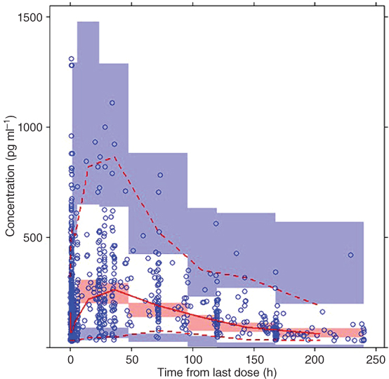
Figure 18.1 Final pharmacokinetic model visual predictive check. Solid line represents median values of observed data; dashed line represents median values of simulated data; circles represent observed data; shaded area represents [2.5th, 97.5th] confidence interval of the 2.5th, median, and 97.5th percentiles of the simulated data. (See insert for color representation of this figure.)
Source: Adapted from Hu et al. 2017 [48] .
Table 18.1 Peginterferon beta‐1a population PK parameter estimates based on nonparametric bootstrap (n = 1000).
| NONMEM output | Bootstrap result | |||||
| Parameter | Definition | Estimated value | Relative standard error (%) | Shrinkage (%) | Valuesa | (2.5th, 97.5th) Percentile |
| θ1 (l h−1) | Typical value of CL | 3.28 | 4.8 | NA | 3.26 | [2.96, 3.52] |
| θ2 (l) | Typical value of V | 435 | 8.1 | NA | 440 | [355, 535] |
| θ3 | Exponent of BMI as a covariate of clearance | 0.779 | 19 | NA | 0.770 | [0.548, 1.11] |
| θ4 | Coefficient of BMI as a covariate of V | 0.0353 | 26 | NA | 0.0353 | [0.0163, 0.0456] |
| θ5 (h−1) a | Difference between absorption rate and elimination rate | 0.207 | 9.8 | NA | 0.210 | [0.164, 0.257] |
| IIV of CL | 0.145 | 19 | 63 | 0.138 | [0.0490, 0.336] | |
| ω2V | IIV of V | 0.352 | 13 | 57 | 0.346 | [0.182, 0.472] |
| SD | Standard deviation of random error | 0.566 | 2.4 | 0.564 | [0.534, 0.608] | |
| σ2 | Additive random error for log‐transformed data | 1, fixed | NA | 14 | 1, fixed | NA |
aθ5, Ka−Ke; Ka, absorption rate; Ke, elimination rate.
Source: Adapted from Hu et al. 2017 [48] .
18.2.3 AUC‐Gd+ Lesion Count Model for Peginterferon Beta‐1a
In study ADVANCE, individual Gd+ lesion counts were characterized by large inter‐subject variability, over dispersed distribution (high proportion of both zero counts and high counts), and a decrease with time in the active treatment groups. Different models were tested, including marginal Poisson model, marginal zero‐inflated Poisson (ZIP) model, marginal negative binomial model, mixed effect negative binomial model, and mixture negative binomial model [49] . A log–linear relationship was assumed between monthly cumulative AUC and Gd+ lesion count. All models showed a negative slope between AUC and log(Gd+), indicating the Gd+ lesion count decreased with increasing exposure. Among all models tested, the mixture negative binomial model provided the best description of data. In this model, the population was assumed to come from two distinct subpopulations: a subpopulation with low baseline Gd+ lesion activity and a subpopulation with relatively higher baseline Gd+ lesion activity (denoted by λi0 in Eq. (18.3)).
where Y∼Bernoulli(1, p), ![]() ) and
) and ![]() ).
).
The post‐treatment Gd+ lesion count λij in subject i at time j was described by the following equation.
where tij is the day after first dose of active dose (would be 0 at baseline or for placebo treatment) and t1/2 is the pharmacologic half‐life effect parameter to be estimated.
The observed Gd+ lesion count was modeled using negative binomial distribution as described in Eq. (18.5).

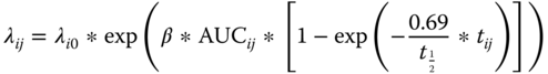
where x is the random variable for lesion count, k is an observed outcome, λij is the mean, and r is a parameter reflecting over‐dispersion, which may take one of two values, r1 and r2 for the low lesion activity and the higher lesion activity subpopulation, respectively. The VPC is shown in Figure 18.2. The parameter estimates are shown in Table 18.2.
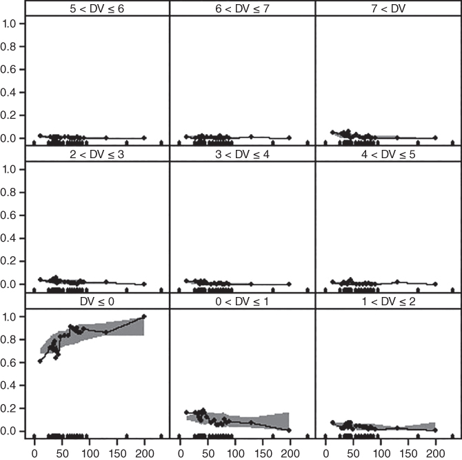
Figure 18.2 Visual predictive check for marginal probability of different lesion count categories (0, 1, 2, 3, 4, 5, 6, 7, and >7 counts) based on 1000 simulations with the mixture negative binomial model. The Gd+ lesion count observations were divided into 21 groups according to associated AUCss (one group for zero AUCss and 20 groups for all positive AUCss). The dots connected by a line were the observed proportion for different lesion count categories and the shaded region were the corresponding 90% CI based on simulation. The dots along the x‐axis are the boundary value of each AUC bin. CI, confidence interval; Gd+, gadolinium‐enhanced; SC, subcutaneous.
Source: Adapted from Hang et al. 2016 [49] .
Table 18.2 Parameter estimates of the AUC‐Gd + lesion count mixture negative binomial model based on nonparametric bootstrap (n = 500).
| NONMEM output | Bootstrap result | |||||
| Model parameter | Description | Estimated value | Relative standard error (%) | Shrinkage (%) | Median | 95% CI |
| λ0_1 | Baseline mean Gd+ lesion count for a typical subject in the lower baseline lesion activity subpopulation | 0.48 | 11.8 | NA | 0.474 | [0.382, 0.609] |
| R | Ratio of the mean Gd+ lesion count for a typical subject in higher baseline lesion activity group to lower baseline lesion activity group | 3.53 | 12.2 | NA | 3.58 | [2.58, 4.73] |
| λ0_2 | Baseline mean Gd+ lesion count for a typical subject in the higher baseline lesion activity subpopulation (parameterized as λ0_1 × R) | 1.69 | NA | NA | 1.70 | NA |
| r1 | Dispersion parameter for baseline λ in the lower baseline lesion activity subpopulation | 44.8 | 6.2 | NA | 44.7 | [39.6, 50.8] |
| r2 | Dispersion parameter for baseline λ in the higher baseline lesion activity subpopulation | 0.499 | 9.1 | NA | 0.496 | [0.398, 0.586] |
| α | Logit of proportion of lower baseline lesion activity subpopulation | 0.415 | 22.3 | NA | 0.413 |
[0.246, 0.624] |
| P | Proportion of subjects with lower baseline lesion activity | 0.602 | NA | NA | 0.602 | [0.561, 0.651] |
| β | Slope of AUC effect on log(λ) | −0.0256 | 8.5 | NA | −0.0257 | [−0.0304, −0.0216] |
| t1/2 | Half‐life of drug effect onset time (days) | 115 | 21.1 | NA | 113.8 | [73.8, 179.6] |
| σ2 | Variance of random effect on baseline λ in log scale for the higher baseline lesion activity subpopulation | 1.25 | 9.2 | 28.4 | 1.22 | [1.00, 1.46] |
AUC, area under the curve; CI, confidence interval; Gd+, gadolinium‐enhanced.
Source: Adapted from Hang et al. 2016 [49] .
The estimated slope of monthly AUC effect on log(λ) is −0.0256, which implied with each additional increase of 27 ng ml−1 × h in AUC, λ was reduced by an additional 50%. Across the every‐two‐week AUC range, the range of decline was much narrower than that across the every‐four‐week AUC range; in addition, the mean decline for the every‐two‐week group was greater than that of the every‐four‐week group. In Figure 18.3, the simulation‐based mean curve is aligned with the central tendency of the observed data and the observed mean lesion counts lie within the simulation‐based 95% CI. Similar marginal mean lesion count was observed across the range of AUC resulting from the every‐two‐week regimen. However, in the range of every‐four‐week AUC, a substantial difference in marginal mean lesion count between the low AUC subgroup and the high AUC subgroup was demonstrated by both observed data and model predictions.
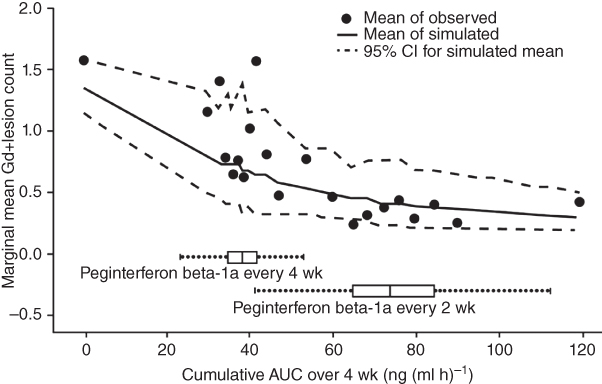
Figure 18.3 Observed marginal mean Gd+ lesion count by AUC subgroup, overlaid with mean and 95% CI based on 1000 simulations. Boxplot represents monthly AUC based on population PK model in the every‐two‐weeks and every‐four‐weeks arms.
Source: Adapted from Hang et al. 2016 [49] .
18.2.4 AUC‐T2 Lesion Count Model for Peginterferon Beta‐1a
Similar models were tested on the longitudinal T2 lesion count data, and the relative performance of these models in terms of goodness‐of‐fit were in the same order as for Gd+ lesion count data [49] . The final model selected to describe T2 lesion count data was also a Mixture Negative Binomial model with two subpopulations for the between‐subject variation on baseline mean parameter λi0. The parameter estimates are shown in Table 18.3. The effect of AUC on log(λ) is estimated to be −0.0147, which suggested that increased AUC led to a greater reduction of T2 lesion count. Figure 18.4 shows that the model fits the data well and a smaller difference in T2 lesion count was observed among subjects receiving the every‐two‐week regimen compared to the every‐four‐week regimen, consistent with the AUC‐Gd+ lesion model.
Table 18.3 Parameter estimates of the AUC‐T2 lesion count mixture negative binomial model based on nonparametric bootstrap (n = 500).
| NONMEM output | Bootstrap result | |||||
| Model parameter | Description | Estimated value | Relative standard error (%) | Shrinkage (%) | Median | 95% CI |
| λ0_1 | Baseline mean T2 lesion count for a typical subject in the lower baseline lesion activity subpopulation | 0.0066 | 15.3 | NA | 0.0065 | (0.0049, 0.0089) |
| R | Ratio of the mean T2 lesion count for a typical subject in higher baseline lesion activity group to lower baseline lesion activity group | 4.71 | 15.8 | NA | 4.81 | (3.48, 6.25) |
| λ0_2 | Baseline mean T2 lesion count for a typical subject in the higher baseline lesion activity subpopulation (parameterized as λ0_1 × R) | 0.031 | NA | NA | 0.031 | NA |
| r1 | Dispersion parameter for baseline λ in the lower baseline lesion activity subpopulation | 35.7 | 7.1 | NA | 35.5 | (30.6, 40.6) |
| r2 | Dispersion parameter for baseline λ in the higher baseline lesion activity subpopulation | 0.459 | 6.3 | NA | 0.454 | (0.396, 0.518) |
| α | Logit of proportion of lower baseline lesion activity subpopulation | 14.2 | NA | −0.605 | (−0.778, −0.432) | |
| P | Proportion of subjects with lower baseline lesion activity | 0.354 | NA | 0.353 | (0.315, 0.394) | |
| β | Slope of AUC effect on log(λ) | −0.0147 | 7.4 | NA | −0.0147 | (−0.0170, −0.0124) |
| σ2 | Variance of random effect on baseline λ in log scale for the higher baseline lesion activity subpopulation | 1.21 | 7.2 | 20.3 | 1.22 | (1.05, 1.39) |
AUC, area under the curve; CI, confidence interval.
Source: Adapted from Hang et al. 2016 [49] .
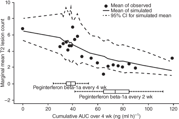
Figure 18.4 Observed marginal mean new or newly enlarged T2 lesion count by monthly AUC subgroup, overlaid with mean and 95% CI based on 1000 simulations.
Source: Adapted from Hang et al. 2016 [49] .
18.2.5 AUC–ARR Model for Peginterferon Beta‐1a
Four models were explored to describe the relapse count data, including Poisson, zero‐inflated‐Poisson, log‐Poisson, and Poisson‐gamma (negative binomial) models [48] . The Poisson‐gamma model provided the best fit to the data. In the model, the relapse count for subject i, the observed relapse counts, nrelapse, i was modeled using Poisson distribution (Eq. (18.6)) with a mean of λi · ti, where λi represents the mean ARR for subject i and ti represents treatment duration for subject i.
λi was assumed to follow gamma distribution as shown in Eq. (18.7), where α represents shape factor and ![]() represents typical population ARR with a specific AUCi.
represents typical population ARR with a specific AUCi.

The effect of drug exposure was evaluated as shown by Eq. (18.8), where ![]() represents mean ARR for subject i with AUCi, λ0 represents population baseline ARR, and b represents coefficient for AUC.
represents mean ARR for subject i with AUCi, λ0 represents population baseline ARR, and b represents coefficient for AUC.
The following covariates were tested, namely, baseline expanded disability status scale (EDSS) scores (scores from 0 [normal] to 10 [death due to MS] with a step 0.5 to grade the degree of neurologic impairment in MS) [50], baseline relapse rate (mean relapse counts in the three years before study entry), age, sex, baseline McDonald criteria (a score of 1–4 based on number of relapses and MRI lesions; modeled both categorically and continuously), and baseline Gd+ lesion volume. The covariate was modeled using a log–linear relationship shown in Eq. (18.9).
where c represents the covariate coefficient and Pi represents the covariate value for subject i. No covariate yielded better model fit and Eq. ( 18.8 ) represents the final model.
The parameter estimates are shown in Table 18.4. A negative slope for AUC (b = −0.00532 1/[ng ml × h × yr]) confirmed that ARR decreased as cumulative AUC increased.
Table 18.4 Summary of AUC‐relapse model parameter estimates.
| NONMEM output | Bootstrap result | |||||
| Model parameter | Mean | SD | Time‐series SE | Median | 2.50% | 97.50% |
| λ0 (1 y−1) | 0.37 | 0.0277 | 0.00104 | 0.369 | 0.318 | 0.427 |
| α | 0.795 | 0.121 | 0.00615 | 0.782 | 0.593 | 1.06 |
| b (1 [ng/ml × h × y]−1) | −0.00532 | 0.00148 | 6.17E−05 | −0.00531 | −0.00827 | −0.00237 |
SD, standard deviation; SE, standard error.
Source: Adapted from Hu et al. 2017 [48] .
Comparison between simulated and observed data showed the alignment between the observed and the model‐predicted ARR (Figure 18.5). In the AUC stratified plot, the slope for ARR reduction in the plot was steep in the every‐four‐weeks AUC range, especially below the group median AUC. In contrast, the slope started to level off in the every‐two‐weeks AUC range. This trend was consistent between the observed and the model‐predicted data.
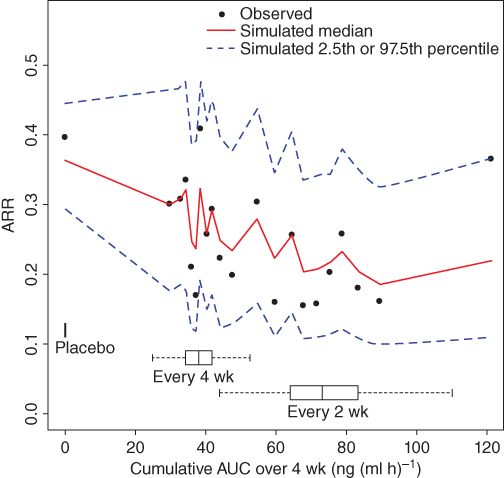
Figure 18.5 Comparison of observed and simulated data for the AUC‐ARR model. Peginterferon beta‐1a treated subjects were pooled and divided into 20 subgroups with each subgroup containing 5 percentiles (approximately 50 patients) of monthly cumulatively AUC. AUC, area under the curve; ARR, annualized relapse rate, calculated as the cumulative relapse count divided by the cumulative treatment time within the subgroup and normalized over 365.25 days.
Source: Adapted from Hu et al. 2017 [48] .
Based on the median model parameter estimates, the median AUCs of the every‐four‐weeks (38.0 ng (ml × h)−1) and every‐two‐weeks groups (73.1 ng (ml × h)−1) were associated with ARR reductions of 18% and 32%, respectively, compared with the placebo group.
18.2.6 Label Recommendation
The AUC‐Gd+ lesion, AUC‐T2 lesion, and AUC‐ARR models all showed that a large proportion of subjects with low peginterferon beta‐1a exposure in the every‐four‐weeks group had suboptimal efficacy, providing more insight into the recommended every‐two‐weeks dosing regimen. Given that the every‐two‐weeks and every‐four‐weeks groups showed similar safety profiles [ 46 , 47 ], and that a large proportion of subjects received suboptimal exposure with every‐four‐weeks dosing, every‐two‐weeks was the only proposed dosing regimen, and the recommendation was adopted in the FDA and EMA labels [51,52].
18.3 Population PK/PD Analyses of Daclizumab Beta and Phase 3 Dose Selection
Daclizumab beta (formerly, daclizumab high‐yield process, approved as ZINBRYTA®, which has a different form and structure than an earlier form of daclizumab) is a humanized IgG1 monoclonal antibody that binds specifically to the alpha subunit (CD25) of the human high‐affinity interleukin (IL)‐2 receptor (IL‐2R) that is expressed on the surface of activated lymphocytes [53], inhibiting CD25‐dependent, high‐affinity IL‐2 receptor signaling, but leaving intermediate‐affinity IL‐2 receptor signaling intact [54]. This signaling modulation results in several well‐characterized immunologic changes, including an expansion of immunoregulatory CD56bright natural killer (NK) cells [55–58], which kill autologous activated T cells, inhibition of T‐cell activation by dendritic cells [59–61], and a reduction in lymphoid tissue inducer cells, which are typically increased in MS patients [62,63]. These effects have been associated with the therapeutic effect of daclizumab beta to treat MS. In a 52‐week Phase 2 study (SELECT), MS patients were treated with 150 mg (n = 208) or 300 mg (n = 209) SC daclizumab beta, with placebo control (n = 204). There was a 54% (95% CI 33–68%; p < 0.0001) reduction in ARR in the 150 mg treatment group, and 50% reduction (28–65%; p = 0.00015) in the 300 mg group, compared to placebo treatment. Similar safety profiles were observed, with serious adverse events excluding MS relapse observed in 12 (6%), 15 (7%), and 19 (9%) patients in the placebo group, 150 mg group, and 300 mg group, respectively. Based on the PK and pharmacodynamics (PDs) results, 150 mg every‐four‐week dosing regimen was selected in Phase 3 studies and proved efficacious with acceptable safety profiles [58] . Population PK and PK/PD modeling were carried out to guide dose selection through drug development. The final PK and PK/PD models supported 150 mg every four weeks dosing regimen.
18.3.1 Daclizumab Beta Population PK Model
A population PK model was built using data from Phase 1 through Phase 3 studies [64]. A two‐compartment model with first‐order absorption and elimination adequately described daclizumab beta pharmacokinetics. CL was 0.212 l d−1 and the central volume of distribution was 3.92 l, both scaled by [body weight (kg)/68] with exponents of 0.87 and 1.12, respectively. The peripheral volume of distribution was 2.42 l and the intercompartmental clearance was 0.977 l d−1. Absorption lag time, mean absorption time, and absolute bioavailability (100–300 mg SC) were 1.61 h, 7.2 days, and 88%, respectively. The daclizumab beta terminal half‐life was 21 days. Baseline CD25, age, and sex did not influence daclizumab beta PK, which was reflected in the label [65]. Body weight explained 37% and 27% of the IIV for CL and central volume of distribution, respectively. The Neutralizing antibody (NAb) positive status (6.1% at any time) increased daclizumab beta CL by 19%.
18.3.2 PK/PD Model
Several PD responses have been explored in daclizumab beta MS studies based on their relationship to IL‐2 signaling modulation [66,67]. In clinical studies of MS subjects, the PD responses observed included sustained CD25 saturation on peripheral T cells, a decrease in regulatory T cells (Treg) and an increase in serum IL‐2 and CD56bright NK cells during daclizumab beta Treatment. T cell and B cell counts decreased ≤10% from baseline during the first year of daclizumab beta treatment, while total NK cell counts increased approximately 1.5‐fold as a result of the change in CD56bright NK cells [66] . As key PD markers, CD25 occupancy, CD56bright NK cell expansion, and regulatory T cell reduction were measured and modeled using data from MS patients [67] . The CD25 occupancy on peripheral CD4+ T cells was modeled using Eq. (18.10). Because target T cells were in the blood stream instead of in tissues, binding of daclizumab beta in the circulation to CD25 was considered an instantaneous effect. A sigmoidal maximum response (Emax) model was utilized to characterize unoccupied CD25 (denoted as CD25 in Eq. ( 18.10 )) on peripheral T cells in subjects with RRMS upon treatment with daclizumab beta.
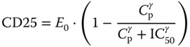
where E0 represents unoccupied CD25 at baseline, Cp represents serum daclizumab beta concentration, γ represents Hill coefficient, IC50 represents serum daclizumab beta concentrations to achieve 50% of baseline unoccupied CD50. Since the OBSERVE intensive sub‐study contained the most informative sampling schedule about the saturation phase of CD25 occupancy, OBSERVE intensive data were singled out to characterize the saturation of CD25 occupancy by daclizumab beta. However, the PD model estimates from the OBSERVE intensive data cannot describe well the desaturation phase for the SELECTION washout period. In the final model (Table 18.5), the Hill coefficient (γ) and IC50 for the saturation phase were fixed as those from OBSERVE intensive data and for the SELECTION washout desaturation phase, separate Hill coefficients and IC50 were estimated.
Table 18.5 PD model parameter estimate summary for daclizumab HYP.
| NONMEM output | Bootstrap result | |||||
| PD model | Parameter | Estimated value | Relative standard error (%) | Shrinkage (%) | Median | 95% CI |
| CD25 occupancy model | Baseline E0 (%) | 56 | 0.57 | NA | 56 | (55, 56) |
| IIV (additive) | 11 | NA | 10.4 | 11 | (10, 11) | |
| Saturation IC50 (mg l−1) | 0.0135 (fixed) | NA | NA | 0.0135 (fixed) | NA | |
| Saturation Hill coefficient | 1 (fixed) | NA | NA | 1 (fixed) | NA | |
| CD56bright NK cell expansion model | Kin (%/h) | 4.12E‐04 | 6.92 | NA | 4.1E−04 | (3.7E−04, 4.5E−04) |
| IIV (%) | 97 | NA | 25 | 97 | (90, 104) | |
| Smax | 7.89 | 9.59 | NA | 7.88 | (7.12, 8.89) | |
| IIV (%) | 67 | 10.6 | 67 | (64, 71) | ||
| IC50 (mg l−1) | 18.0 | 22.4 | NA | 17.8 | (14.2, 22.8) | |
| Residual error (proportional; %) | 29.1 | NA | 9.7 | 29.0 | (28.2, 29.9) | |
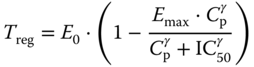
| Treg reduction model | Baseline E0 (%) | 12.1 | 1.68 | NA | 12.2 | (11.8, 12.6) |
| IIV (%) | 42 | NA | 15.6 | 42 | (39, 44) | |
| IC50 (mg l−1) | 3.97 | 8.51 | NA | 3.98 | (3.34, 4.66) | |
| IIV (%) | 65 | NA | 60.5 | 63 | (46, 78) | |
| Hill coefficient | 2 | 28 | NA | 1.92 | (1.39, 2.91) | |
| Emax | 0.610 | 4.02 | NA | 0.614 | (0.584, 0.654) | |
| IIV (%) | 12 | NA | 57.7 | 12 | (9, 14) | |
| Residual error (proportional; %) | 50.1 | NA | 6.1 | 50.2 | (48.8, 51.2) | |
| Residual error (additive) | 0.416 | NA | 6.1 | 0.420 | (0.154, 0.628) | |
Source: Adapted from Diao et al. [67] .
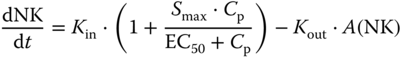
Expansion of CD56bright NK cells by daclizumab beta was hypothesized through the increased availability of T cell‐derived IL‐2 for NK cell signaling [15] and was modeled using an indirect stimulatory Smax function on the zero‐order rate Kin of production of NK cells (Eq. (18.11)). In the equation, Kout is the first‐order rate constant for elimination of CD56bright NK cells, Cp denotes daclizumab beta serum concentration and Smax is the maximum stimulatory factor attributed to daclizumab beta as shown in Eq. (18.12).
The Treg count was modeled using a sigmoidal Emax model.
The VPC for the PK and PD models for SELECT/SELECTION and OBSERVE is shown in Figures 18.6–18.9. Model estimates are shown in Table 18.5 .
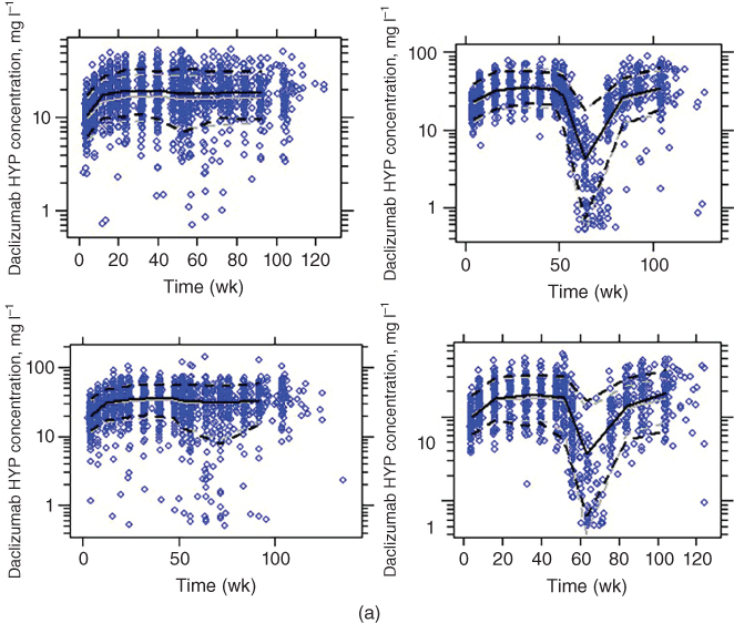
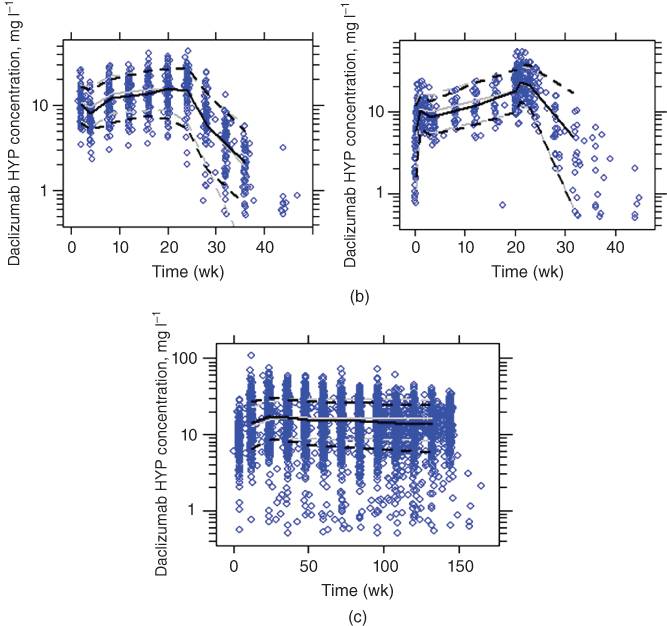
Figure 18.6 Visual predictive check of the PK model (solid line, median; dotted line, 10th and 90th percentiles; black lines, observed; gray lines, simulated; grey dots, observed). (a) Select/selection (upper left: 150 mg no washout; upper right: 150 mg washout; lower left: 300 mg no washout; lower right: 300 mg washout). (b) Observe (left: intensive; right: less‐intensive). (c) Decide (using the model developed excluding this Phase 3 study).
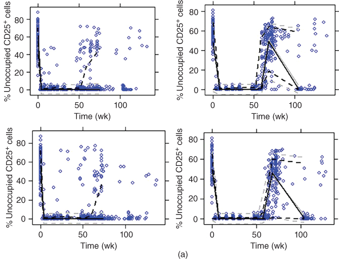

Figure 18.7 Visual predictive check for CD25 occupancy model (solid line, median; dotted line, 10th and 90th percentiles; black lines, observed; gray lines, simulated; dots, observed). (a) Select/selection (upper left: 150 mg no washout; upper right: 150 mg washout; lower left: 300 mg no washout; lower right: 300 mg washout). (b) Observe (left: intensive; right: nonintensive). (c) Decide.
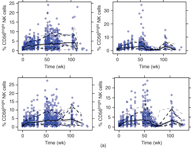
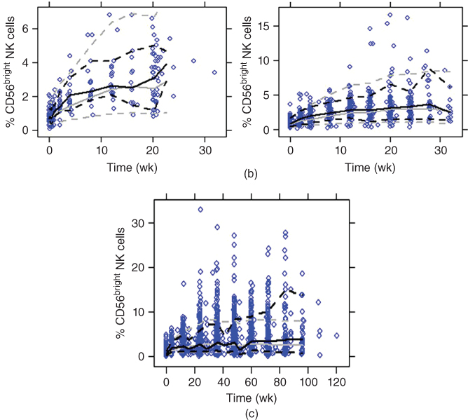
Figure 18.8 Visual predictive check for CD56bright NK cell expansion model (solid line, median; dotted line, 10th and 90th percentiles; black lines, observed; gray lines, simulated; blue dots, observed). (a) Select/selection (upper left: 150 mg no washout; upper right: 150 mg washout; lower left: 300 mg no washout; lower right: 300 mg washout). (b) Observe (left: intensive; right: nonintensive). (c) Decide.
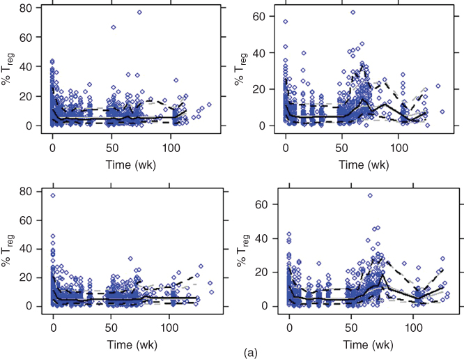

Figure 18.9 Visual predictive check for Treg down‐regulation model (solid line, median; dotted line, 10th and 90th percentiles; black lines, observed; gray lines, simulated; blue dots, observed). (a) Select/selection (upper left: 150 mg no washout; upper right: 150 mg washout; lower left: 300 mg no washout; lower right: 300 mg washout). (b) Observe (left: intensive; right: nonintensive). (c) Decide.
18.3.3 Simulation in Support of Phase 3 Dose Selection
Using the PK and PD model, CD25 occupancy, NK cell expansion, and Treg reduction were simulated following every four weeks SC dosing regimen at 150 and 300 mg and are presented in Figure 18.10. Upon daclizumab beta treatment, CD25 saturation was rapid with complete saturation occurring after approximately seven hours and maintained when daclizumab beta serum concentration was ≥5 mg l−1 throughout the treatment for 150 or 300 mg SC every four weeks; NK cell expansion plateaus approximately at Week 36, at which the average maximum expansion ratio is 5.2 and 6.5, for the 150 and 300 mg treatment groups, respectively; Treg reduction was characterized by a sigmoidal Emax model. Average maximum reduction of 56% and 60% occurred approximately four days post 150 and 300 mg SC dose, respectively. The simulations showed similar PD profiles between 150 and 300 mg SC dosing regimens, despite a twofold differences in systemic exposure. The PK/PD simulations supported the approved dosing regimen of 150 mg SC once monthly. Previously, a lower dose 1 mg kg−1 was tested in a Ph2 add‐on trial with interferon beta and was found not as efficacious [56].
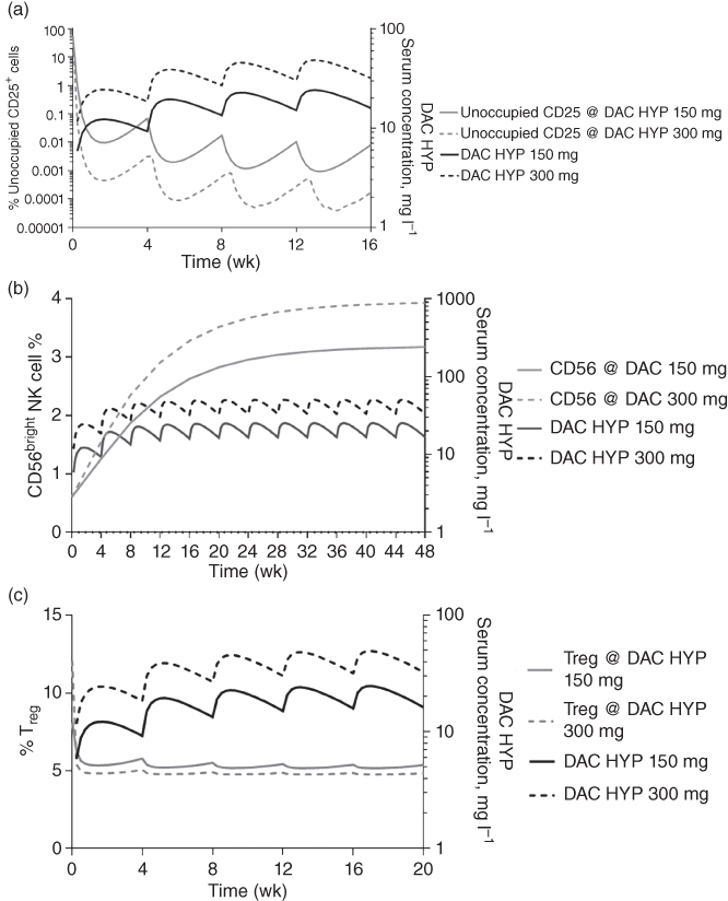
Figure 18.10 Simulated (a) CD25 occupancy profile, (b) CD56bright NK cell percent, (c) Treg percent at steady state following daclizumab beta SC at 150 mg or 300 mg every four weeks.
Source: Adapted from Diao et al. [67] .
18.4 Model‐Based Approach for the Clinical Development of Subcutaneous Natalizumab
Natalizumab, a recombinant humanized monoclonal antibody, binds to the α4‐subunit of α4β1 and α4β7 expressed on the surface of all leukocytes except neutrophils, and inhibits the α4 mediated adhesion of leukocytes to their counter‐receptor(s). The receptors for the α4 family of integrins include vascular cell adhesion molecule‐1 (VCAM‐1), which is expressed on activated vascular endothelium, and mucosal addressin cell adhesion molecule‐1 (MAdCAM‐1) present on vascular endothelial cells of the gastrointestinal tract. Disruption of these molecular interactions prevents transmigration of leukocytes across the endothelium into inflamed parenchymal tissue and prevents their activation by ligands in the parenchyma [68,69]. By inhibiting or preventing leukocyte entry into the CNS and subsequent leukocyte activation, natalizumab slowed MS progression and reduced relapsed rate when compared to placebo or interferon beta‐1a treatment in two controlled registration studies [ 69 ,70]. The current approved natalizumab clinical dose (300 mg) is administered by intravenous (IV) infusion over duration of one hour every four weeks. A new SC formulation of natalizumab has been under development as a possible alternative to IV administration. The SC dose bridging was based on the assumption that after the completion of SC absorption phase, comparable natalizumab trough concentration would result in similar target engagement and efficacy, as compared to the approved IV regimen. Both Ctrough and trough α4 integrin binding (%) were selected for comparison based on the observation that binding of α4 integrin was partial at Ctrough, while the binding was almost saturated at Cmax for both IV and SC (>99% of maximum saturation). Although the SC route provided a slow increase to Cmax over several days in contrast to the instantaneous Cmax following IV infusion, the elimination profiles between IV and SC route paralleled each other [56] . Hence, for a SC dose with achieving comparable trough and α4 integrin saturation to 300 mg IV dose, it was assumed that adequate protection from disease activity as IV dose would be achieved.
18.4.1 Pharmacokinetic Model of Natalizumab
Natalizumab pharmacokinetics was described using a two‐compartment model with a combination of first‐order and Michaelis–Menten elimination as shown in Figure 18.11. The SC absorption was characterized using a first‐order absorption and lag time. Linear clearance was affected by anti‐natalizumab antibodies and body weight while central compartment volume was impacted by only body weight. The PK parameter estimates that were used for simulation for SC formulation development are summarized in Table 18.6. Relevant covariate to SC formulation development included body weight for clearance and central volume of distribution.
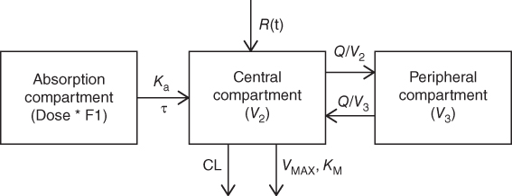
Figure 18.11 Structural model describing natalizumab pharmacokinetics. Note: CL, clearance; Q, distribution clearance; Ka, first‐order absorption rate constant; VMAX, maximum target mediated elimination rate; KM, Michaelis–Menten constant; V2, volume of central compartment; and V3, volume of peripheral compartment; R(t), IV infusion; τ, lag time.
Table 18.6 Parameter estimates of the final natalizumab population pharmacokinetic model based on nonparametric bootstrap (n = 1000).
| NONMEM output | Bootstrap result | ||||
| Parameter | Estimated value | Relative standard error (%) | Shrinkage (%) | Median | 95% CI |
| CL (l h−1) | 0.00625 | 0.000159 | NA | 0.00621 | (0.0056, 0.0067) |
| V2 (l) | 3.76 | 0.05 | NA | 3.75 | (3.65, 3.86) |
| V3 (l) | 1.82 | 0.0519 | NA | 1.83 | (1.62, 2.06) |
| Q (l h−1) | 0.0168 | 0.00127 | NA | 0.0169 | (0.012, 0.0242) |
| VMAX (mg h−1 l−1) | 0.155 | 0.0105 | NA | 0.158 | (0.124, 0.202) |
| KM (mg l−1) | 7.55 | 0.889 | NA | 7.64 | (4.71, 11.7) |
| Parameters relevant to S.C. arm | |||||
| Ka (h−1) | 0.0111 | 0.000878 | NA | 0.0112 | 0.0094–0.130 |
| Lag. time (h) | 3.03 | 0.129 | NA | 3.04 | 2.73–3.46 |
| F (%) | 82.2 | 1.51 | NA | 82.4 | 76.9–87.6 |
| Structural covariate effect | |||||
| Power factor | |||||
| WT on CL | 0.863 | 0.0517 | NA | 0.867 | 0.763–0.968 |
| WT on V2 | 0.292 | 0.0587 | NA | 0.290 | 0.174–0.398 |
| Inter‐individual variability | |||||
| Variance on CL | 0.120 | 0.00650 | 5.34 | 0.119 | 0.105–0.139 |
| Variance on V2 | 0.0751 | 0.00647 | 35.5 | 0.0752 | 0.060–0.091 |
| Variance on KA | 0.121 | 0.0553 | 88.6 | 0.112 | 0.0345–0.209 |
| Covariance on (CL, V2) | 0.0366 | 0.00469 | NA | 0.0368 | 0.027–0.045 |
| Residual variability | |||||
| Proportional error (%) | 0.321 | 0.00346 | 7.01 | 0.321 | 0.312–0.330 |
CL, clearance; V2, central volume of distribution; V3, peripheral volume of distribution; Q, intercompartmental clearance; VMAX, maximum binding rate; KM, concentration at half maximum binding rate; KA, rate of absorption; F, relative bioavailability of S.C. route of administration to I.V. route of administration.
Source: Adapted from Muralidharan et al. 2017 [71].
18.4.2 Natalizumab Pharmacodynamic Model
The relationship between natalizumab concentration and α4 integrin saturation was described using a sigmoidal Emax direct effect model as shown in Eq. (18.13).
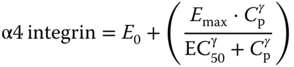
where α4 integrin represents the fraction of α4 integrin saturation, Emax represents maximum binding, Cp is the predicted serum concentration of natalizumab; E0 is the background α4 integrin saturation at baseline; ϒ is the hill coefficient; and EC50 is the concentration of natalizumab that results in 50% of maximum α4 integrin saturation. The parameter estimates are shown in Table 18.7.
Table 18.7 Parameter estimates of the final natalizumab pharmacodynamic model based on nonparametric bootstrap (n = 1000).
| NONMEM output | Bootstrap result | ||||
| Parameter | Estimated value | Relative standard error (%) | Shrinkage (%) | Median | 95% CI |
| Drug effect | |||||
| E0 (%) | 6.64 | 0.350 | NA | 6.62 | 6.20, 7.07 |
| EMAX (%) | 83.8 | 0.918 | NA | 83.8 | 81.9, 86.6 |
| EC50 (mg l−1) | 2.51 | 0.0799 | NA | 2.51 | 2.25, 2.94 |
| Hill | 1.35 | 0.0777 | NA | 1.34 | 1.14, 1.56 |
| Covariate effect | |||||
| Age on EMAX | 0.249 | 0.0253 | NA | 0.249 | 0.181, 0.330 |
| Age on Hill | −1.090 | 0.135 | NA | −1.09 | −1.50, −0.702 |
| Inter‐individual variability | |||||
| Variance on EMAX | 0.0119 | 0.00124 | 25.0 | 0.0116 | 0.008, 0.015 |
| Variance on Hill | 0.238 | 0.0310 | 32.3 | 0.231 | 0.151, 0.331 |
| Residual variability | |||||
| Additive error (%) | 9.72 | 0.121 | 7.66 | 9.73 | 9.26, 10.2 |
E0, baseline % α4 integrin saturation; EMAX, maximum of α4 integrin saturation; EC50, natalizumab serum concentration at 50% of maximum saturation; Hill, shape factor.
Source: Adapted from Muralidharan et al. 2017 [71] .
18.4.3 Simulation for Natalizumab SC Dose Selection
To determine a SC dose, steady‐state serum natalizumab concentrations and α4 integrin saturation over time were simulated using the above PK–PD model across three different SC doses (300, 325, 350 mg every four weeks), which were then compared to the reference clinically approved 300 mg IV every four weeks to identify the natalizumab SC dose to achieve comparable serum trough concentrations and α4 integrin saturation. The median natalizumab concentration and α4 integrin binding are shown in Figure 18.12, and the distribution of the trough concentrations are shown in Figure 18.13. The PK–PD profiles following six months dosing was simulated to approximate steady state profile because further changes due to nonlinear Michaelis–Menten elimination was minimal.
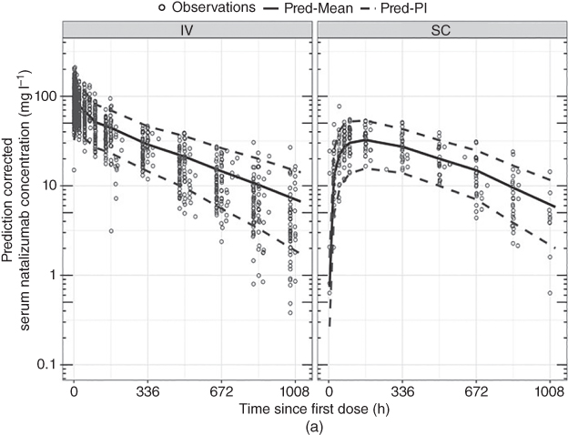
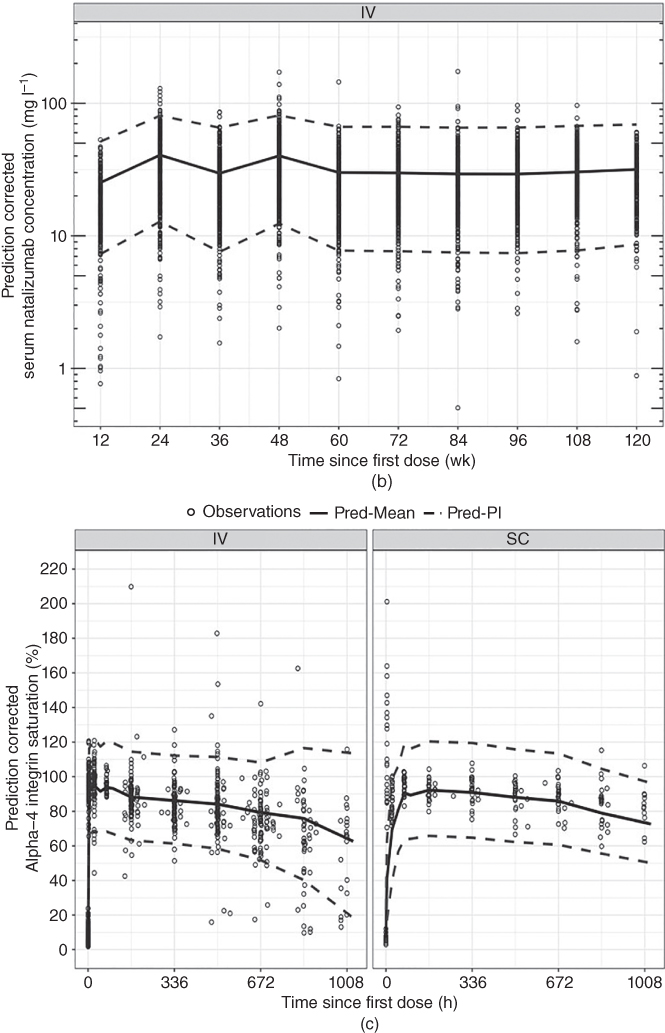
Figure 18.12 Prediction‐corrected visual predictive check for the concentration–time after‐dose profiles of natalizumab (single and multiple doses) and α4‐integrin saturation. The prediction‐corrected serum natalizumab concentrations are on a log scale. Open circle: individual observations; solid line: the predicted mean dotted lines: the 95% prediction interval. Pred‐Mean, predicted mean; Pred‐PI, predicted prediction interval.
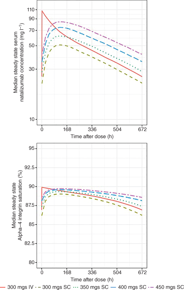
Figure 18.13 Simulated natalizumab PK and PD profiles at steady state.
As shown by simulations, 300 mg every four week SC treatment yielded comparable trough serum natalizumab concentration and trough α4 integrin saturation relative to the reference 300 mg every four week IV dose at steady state. Minimal differences in simulated trough natalizumab concentrations and α4 integrin saturations were observed across the subpopulations between IV and SC route of administrations at the 300 mg (Figure 18.14). Simulated steady‐state mean Ctrough (5th, 95th) percentile was 29.0 (9.64, 61.6) mg l−1 with 300 mg every four weeks IV administration vs. 24.1 (8.95, 44.8) mg l−1 with 300 mg every four weeks SC administration; this corresponded to similar trough α4 integrin saturation, 84.8% (67.4%, 102%) for 300 mg every four weeks IV, and 83.9% (67.4%, 100%) for 300 mg every four weeks SC. Collectively, from these simulations, it was inferred that administering subjects with a 300 mg every‐4‐week SC dose provided comparable α4 integrin saturation at steady state as the clinically approved 300 mg every‐4‐week IV administration.
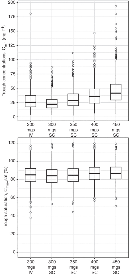
Figure 18.14 Distribution of simulated natalizumab steady‐state PK–PD parameters. Boxes indicate the interquartile range and the whiskers indicate the range excluding the outliers. Open circles represent outliers which are greater than or lesser than 1.5 times the value of first or third quartile. The horizontal line within each box represents the median. Cavg is defined as AUCtau/tau with tau being 672 hours. Ctrough is the minimum natalizumab serum concentration or α4‐integrin saturation.
18.5 Summary
Three examples were given to show case how QCP was used in support of the development of therapeutic proteins for MS. To establish an exposure–response model, the exposure could be represented by AUC, instantaneous concentration, or trough concentration; the response could be selected based on clinical endpoints, or early biological response PD markers. In principle, selection of models should be based on MOA and consideration for model application. With more understanding of MS as an auto‐immune disease, QCP will provide more support during drug development, hopefully reducing drug candidate attrition and shorten development timeline.
References
- 1 Orton, S.M., Herrera, B.M., Yee, I.M. et al. (2006). Sex ratio of multiple sclerosis in Canada: a longitudinal study. Lancet Neurol. 5 (11): 932–936.
- 2 Kister, I., Chamot, E., Salter, A.R. et al. (2013). Disability in multiple sclerosis: a reference for patients and clinicians. Neurology 80 (11): 1018–1024.
- 3 Mayr, W.T., Pittock, S.J., McClelland, R.L. et al. (2003). Incidence and prevalence of multiple sclerosis in Olmsted County, Minnesota, 1985–2000. Neurology 61 (10): 1373–1377.
- 4 Hersh, C.M. and Fox, R.J. (2015). Multiple sclerosis. http://www.clevelandclinicmeded.com/medicalpubs/diseasemanagement/neurology/multiple_sclerosis/ (accessed 09 January 9 2017).
- 5 European Medicines Agency (2015). Guideline on clinical investigation of medicinal products for the treatment of multiple sclerosis. http://www.thehumanmotioninstitute.org/sites/default/files/WC500185161.pdf (accessesd 22 October 2015).
- 6 Frischer, J.M., Bramow, S., Dal‐Bianco, A. et al. (2009). The relation between inflammation and neurodegeneration in multiple sclerosis brains. Brain 132 (Pt. 5): 1175–1189.
- 7 Fischer, M.T., Sharma, R., Lim, J.L. et al. (2012). NADPH oxidase expression in active multiple sclerosis lesions in relation to oxidative tissue damage and mitochondrial injury. Brain 135 (Pt. 3): 886–899.
- 8 van den Elskamp, I.J., Boden, B., Dattola, V. et al. (2010). Cerebral atrophy as outcome measure in short‐term phase 2 clinical trials in multiple sclerosis. Neuroradiology 52 (10): 875–881.
- 9 Altmann, D.R., Jasperse, B., Barkhof, F. et al. (2009). Sample sizes for brain atrophy outcomes in trials for secondary progressive multiple sclerosis. Neurology 72 (7): 595–601.
- 10 Nourbakhsh, B., Nunan‐Saah, J., Maghzi, A.H. et al. (2016). Longitudinal associations between MRI and cognitive changes in very early MS. Mult. Scler. Relat. Disord. 5: 47–52.
- 11 Modica, C.M., Bergsland, N., Dwyer, M.G. et al. (2016). Cognitive reserve moderates the impact of subcortical gray matter atrophy on neuropsychological status in multiple sclerosis. Mult. Scler. 22 (1): 36–42.
- 12 Fox, R.J. (2008). Picturing multiple sclerosis: conventional and diffusion tensor imaging. Semin. Neurol. 28 (4): 453–466.
- 13 Filippi, M. and Rocca, M.A. (2013). Present and future of fMRI in multiple sclerosis. Expert Rev. Neurother. 13 (12 Suppl.): 27–31.
- 14 Amann, M., Papadopoulou, A., Andelova, M. et al. (2015). Magnetization transfer ratio in lesions rather than normal‐appearing brain relates to disability in patients with multiple sclerosis. J. Neurol. 262 (8): 1909–1917.
- 15 Petracca, M., Vancea, R.O., Fleysher, L. et al. (2016). Brain intra‐ and extracellular sodium concentration in multiple sclerosis: a 7 T MRI study. Brain 139 (Pt. 3): 795–806.
- 16 Cotton, F., Weiner, H.L., Jolesz, F.A. et al. (2003). MRI contrast uptake in new lesions in relapsing–remitting MS followed at weekly intervals. Neurology 60 (4): 640–646.
- 17 Rudick, R.A., Lee, J.C., Simon, J. et al. (2006). Significance of T2 lesions in multiple sclerosis: a 13‐year longitudinal study. Ann. Neurol. 60 (2): 236–242.
- 18 Kappos, L., Moeri, D., Radue, E.W. et al. (1999). Predictive value of gadolinium‐enhanced magnetic resonance imaging for relapse rate and changes in disability or impairment in multiple sclerosis: a meta‐analysis. Gadolinium MRI Meta‐analysis Group. Lancet 353 (9157): 964–969.
- 19 Miller, D.H. (2004). Biomarkers and surrogate outcomes in neurodegenerative disease: lessons from multiple sclerosis. NeuroRx 1 (2): 284–294.
- 20 Sormani, M.P., Bonzano, L., Roccatagliata, L. et al. (2009). Magnetic resonance imaging as a potential surrogate for relapses in multiple sclerosis: a meta‐analytic approach. Ann. Neurol. 65 (3): 268–275.
- 21 Sormani, M.P., Bonzano, L., Roccatagliata, L. et al. (2010). Surrogate endpoints for EDSS worsening in multiple sclerosis. A meta‐analytic approach. Neurology 75 (4): 302–309.
- 22 Bagnato, F., Jeffries, N., Richert, N.D. et al. (2003). Evolution of T1 black holes in patients with multiple sclerosis imaged monthly for 4 years. Brain 126 (Pt 8): 1782–1789.
- 23 Barkhof, F. (1999). MRI in multiple sclerosis: correlation with expanded disability status scale (EDSS). Mult. Scler. 5 (4): 283–286.
- 24 Bitsch, A., Kuhlmann, T., Stadelmann, C. et al. (2001). A longitudinal MRI study of histopathologically defined hypointense multiple sclerosis lesions. Ann. Neurol. 49 (6): 793–796.
- 25 Truyen, L., van Waesberghe, J.H., van Walderveen, M.A. et al. (1996). Accumulation of hypointense lesions (“black holes”) on T1 spin‐echo MRI correlates with disease progression in multiple sclerosis. Neurology 47 (6): 1469–1476.
- 26 Giorelli, M., Livrea, P., Defazio, G. et al. (2001). IFN‐beta1a modulates the expression of CTLA‐4 and CD28 splice variants in human mononuclear cells: induction of soluble isoforms. J. Interferon Cytokine Res. 21 (10): 809–812.
- 27 Kawanokuchi, J., Mizuno, T., Kato, H. et al. (2004). Effects of interferon‐beta on microglial functions as inflammatory and antigen presenting cells in the central nervous system. Neuropharmacology 46 (5): 734–742.
- 28 Liu, Z., Pelfrey, C.M., Cotleur, A. et al. (2001). Immunomodulatory effects of interferon beta‐1a in multiple sclerosis. J. Neuroimmunol. 112 (1–2): 153–162.
- 29 Schreiner, B., Mitsdoerffer, M., Kieseier, B.C. et al. (2004). Interferon‐beta enhances monocyte and dendritic cell expression of B7‐H1 (PD‐L1), a strong inhibitor of autologous T‐cell activation: relevance for the immune modulatory effect in multiple sclerosis. J. Neuroimmunol. 155 (1–2): 172–182.
- 30 Shapiro, S., Galboiz, Y., Lahat, N. et al. (2003). The ‘immunological‐synapse’ at its APC side in relapsing and secondary‐progressive multiple sclerosis: modulation by interferon‐beta. J. Neuroimmunol. 144 (1–2): 116–124.
- 31 Ahn, J., Feng, X., Patel, N. et al. (2004). Abnormal levels of interferon‐gamma receptors in active multiple sclerosis are normalized by IFN‐beta therapy: implications for control of apoptosis. Front. Biosci. 9: 1547–1555.
- 32 Sharief, M.K., Semra, Y.K., Seidi, O.A. et al. (2001). Interferon‐beta therapy downregulates the anti‐apoptosis protein FLIP in T cells from patients with multiple sclerosis. J. Neuroimmunol. 120 (1–2): 199–207.
- 33 Hussien, Y., Sanna, A., Söderström, M. et al. (2001). Glatiramer acetate and IFN‐beta act on dendritic cells in multiple sclerosis. J. Neuroimmunol. 121 (1–2): 102–110.
- 34 Nagai, T., Devergne, O., Mueller, T.F. et al. (2003). Timing of IFN‐beta exposure during human dendritic cell maturation and naive Th cell stimulation has contrasting effects on Th1 subset generation: a role for IFN‐beta‐mediated regulation of IL‐12 family cytokines and IL‐18 in naive Th cell differentiation. J. Immunol. 171 (10): 5233–5243.
- 35 Zang, Y.C., Skinner, S.M., Robinson, R.R. et al. (2004). Regulation of differentiation and functional properties of monocytes and monocyte‐derived dendritic cells by interferon beta in multiple sclerosis. Mult. Scler. 10 (5): 499–506.
- 36 Durelli, L., Conti, L., Clerico, M. et al. (2009). T‐helper 17 cells expand in multiple sclerosis and are inhibited by interferon‐beta. Ann. Neurol. 65 (5): 499–509.
- 37 Pirhonen, J., Sirén, J., Julkunen, I. et al. (2007). IFN‐alpha regulates toll‐like receptor‐mediated IL‐27 gene expression in human macrophages. J. Leukocyte Biol. 82 (5): 1185–1192.
- 38 Shinohara, M.L., Kim, J.H., Garcia, V.A. et al. (2008). Engagement of the type I interferon receptor on dendritic cells inhibits T helper 17 cell development: role of intracellular osteopontin. Immunity 29 (1): 68–78.
- 39 Jensen, J., Krakauer, M., and Sellebjerg, F. (2005). Cytokines and adhesion molecules in multiple sclerosis patients treated with interferon‐beta1b. Cytokine 29 (1): 24–30.
- 40 Muraro, P.A., Leist, T., Bielekova, B. et al. (2000). VLA‐4/CD49d downregulated on primed T lymphocytes during interferon‐beta therapy in multiple sclerosis. J. Neuroimmunol. 111 (1–2): 186–194.
- 41 Muraro, P.A., Liberati, L., Bonanni, L. et al. (2004). Decreased integrin gene expression in patients with MS responding to interferon‐beta treatment. J. Neuroimmunol. 150 (1–2): 123–131.
- 42 Boutros, T., Croze, E., and Yong, V.W. (1997). Interferon‐beta is a potent promoter of nerve growth factor production by astrocytes. J. Neurochem. 69 (3): 939–946.
- 43 Plioplys, A.V. and Massimini, N. (1995). Alpha/beta interferon is a neuronal growth factor. Neuroimmunomodulation 2 (1): 31–35.
- 44 Baker, D.P., Lin, E.Y., Lin, K. et al. (2006). N‐terminally PEGylated human interferon‐beta‐1a with improved pharmacokinetic properties and in vivo efficacy in a melanoma angiogenesis model. Bioconjugate Chem. 17 (1): 179–188.
- 45 Arduini, R.M., Li, Z., Rapoza, A. et al. (2004). Expression, purification, and characterization of rat interferon‐beta, and preparation of an N‐terminally PEGylated form with improved pharmacokinetic parameters. Protein Expression Purif. 34 (2): 229–242.
- 46 Kieseier, B.C., Arnold, D.L., Balcer, L.J. et al. (2015). Peginterferon beta‐1a in multiple sclerosis: 2‐year results from ADVANCE. Mult. Scler. 21 (8): 1025–1035.
- 47 Calabresi, P.A., Kieseier, B.C., Arnold, D.L. et al. (2014). Pegylated interferon beta‐1a for relapsing‐remitting multiple sclerosis (ADVANCE): a randomised, phase 3, double‐blind study. Lancet Neurol. 13 (7): 657–665.
- 48 Hu, X., Hang, Y., Cui, Y. et al. (2017). Population‐based pharmacokinetic and exposure‐efficacy analyses of peginterferon beta‐1a in patients with relapsing multiple sclerosis. J. Clin. Pharmacol. 57 (8): 1005–1016.
- 49 Hang, Y., Hu, X., Zhang, J. et al. (2016). Analysis of peginterferon beta‐1a exposure and Gd‐enhanced lesion or T2 lesion response in relapsing‐remitting multiple sclerosis patients. J. Pharmacokinet. Pharmacodyn. 43 (4): 371–383.
- 50 Kurtzke, J.F. (1983). Rating neurologic impairment in multiple sclerosis: an expanded disability status scale (EDSS). Neurology 33 (11): 1444–1452.
- 51 Food and Drug Administration (2014). PLEGRIDY label. http://www.accessdata.fda.gov/drugsatfda_docs/label/2014/125499lbl.pdf (accessed 22 October 2015).
- 52 European Medicines Agency (2014). PLEGRIDY: EPAR – Product Information. http://www.ema.europa.eu/docs/en_GB/document_library/EPAR_‐_Product_Information/human/002827/WC500170302.pdf (accessed 22 Octorber 2015).
- 53 Waldmann, T.A. (2007). Anti‐Tac (daclizumab, Zenapax) in the treatment of leukemia, autoimmune diseases, and in the prevention of allograft rejection: a 25‐year personal odyssey. J. Clin. Immunol. 27 (1): 1–18.
- 54 Martin, J.F., Perry, J.S., Jakhete, N.R. et al. (2010). An IL‐2 paradox: blocking CD25 on T cells induces IL‐2‐driven activation of CD56(bright) NK cells. J. Immunol. 185 (2): 1311–1320.
- 55 Bielekova, B., Catalfamo, M., Reichert‐Scrivner, S. et al. (2006). Regulatory CD56(bright) natural killer cells mediate immunomodulatory effects of IL‐2Ralpha‐targeted therapy (daclizumab) in multiple sclerosis. Proc. Natl. Acad. Sci. U.S.A. 103 (15): 5941–5946.
- 56 Wynn, D., Kaufman, M., Montalban, X. et al. (2010). Daclizumab in active relapsing multiple sclerosis (CHOICE study): a phase 2, randomised, double‐blind, placebo‐controlled, add‐on trial with interferon beta. Lancet Neurol. 9 (4): 381–390.
- 57 Gold, R., Giovannoni, G., Selmaj, K. et al. (2013). Daclizumab high‐yield process in relapsing–remitting multiple sclerosis (SELECT): a randomised, double‐blind, placebo‐controlled trial. Lancet 381 (9884): 2167–2175.
- 58 Kappos, L., Wiendl, H., Selmaj, K. et al. (2015). Daclizumab HYP versus interferon beta‐1a in relapsing multiple sclerosis. N. Engl. J. Med. 373 (15): 1418–1428.
- 59 Malek, T.R. (2008). The biology of interleukin‐2. Annu. Rev. Immunol. 26: 453–479.
- 60 Wuest, S.C., Edwan, J.H., Martin, J.F. et al. (2011). A role for interleukin‐2 trans‐presentation in dendritic cell‐mediated T cell activation in humans, as revealed by daclizumab therapy. Nat. Med. 17 (5): 604–609.
- 61 Snyder, J.T., Shen, J., Azmi, H. et al. (2007). Direct inhibition of CD40L expression can contribute to the clinical efficacy of daclizumab independently of its effects on cell division and Th1/Th2 cytokine production. Blood 109 (12): 5399–5406.
- 62 Perry, J.S., Han, S., Xu, Q. et al. (2012). Inhibition of LTi cell development by CD25 blockade is associated with decreased intrathecal inflammation in multiple sclerosis. Sci. Transl. Med. 4 (145): 145ra106.
- 63 Rose, J.W. (2012). Anti‐CD25 immunotherapy: regulating the regulators. Sci. Transl. Med. 4 (145): 145fs25.
- 64 Diao, L., Hang, Y., Othman, A.A. et al. (2016). Population pharmacokinetics of daclizumab high‐yield process in healthy volunteers and subjects with multiple sclerosis: analysis of phase I‐III clinical trials. Clin. Pharmacokinet. 55 (8): 943–955.
- 65 Food and Drug Administration (2016). ZINBRYTA label. http://www.accessdata.fda.gov/drugsatfda_docs/nda/2016/761029Orig1s000Lbl.pdf (accessed 09 January 2017).
- 66 Elkins, J., Sheridan, J., Amaravadi, L. et al. (2015). CD56(bright) natural killer cells and response to daclizumab HYP in relapsing‐remitting MS. Neurol. Neuroimmunol. Neuroinflamm. 2 (2): e65.
- 67 Diao, L. et al. (2016). Population PK–PD analyses of CD25 occupancy, CD56bright NK cell expansion, and regulatory T cell reduction by daclizumab HYP in subjects with multiple sclerosis. Br. J. Clin. Pharmacol. 82 (5): 1333–1342.
- 68 Hartung, H.P., Archelos, J.J., Zielasek, J. et al. (1995). Circulating adhesion molecules and inflammatory mediators in demyelination: a review. Neurology 45 (Suppl. 6): S22–S32.
- 69 Polman, C.H., O'Connor, P.W., Havrdova, E. et al. (2006). A randomized, placebo‐controlled trial of natalizumab for relapsing multiple sclerosis. N. Engl. J. Med. 354 (9): 899–910.
- 70 Rudick, R.A., Stuart, W.H., Calabresi, P.A. et al. (2006). Natalizumab plus interferon beta‐1a for relapsing multiple sclerosis. N. Engl. J. Med. 354 (9): 911–923.
- 71 Muralidharan, K.K., Kuesters, G., Plavina, T. et al. (2017). Population pharmacokinetics and target engagement of natalizumab in patients with multiple sclerosis. J. Clin. Pharmacol. 57 (8): 1017–1030.