8.3.1 Full TMDD Model

The full TMDD model equations are described in Section 7.2. Selected details of the NONMEM implementation are presented below.

 $PK         ; PK block
...         ; code to assign model parameters
Ka=THETA(1)*EXP(ETA(1))    ; via THETA and ETA parameters
Base = Ksyn/Kdeg   ; derived parameters
...         ; A_0(4) = Base    ; initial conditions that differ from zero
$DES      ; differential equations block 
DADT(1) = -Ka*A(1)       ; SC depot drug amount
DADT(2) = Ka*A(1)-(Kel+Kpt)*A(2)+Ktp*A(3) ; continued on the next line
   -Kon*A(2)*A(4)+Koff*A(5)*Vc  ; central compartment drug amount
DADT(3) = Kpt*A(1)-Ktp*A(4)     ; tissue compartment drug amount
DADT(4) = Ksyn-Kdeg*A(4)-Kon*A(2)/Vc*A(4)+Koff*A(5) ; target concentration 
DADT(5) = Kon*A(2)/Vc*A(4)‐(Koff+Kint)*A(5) ;drug‐target complex concentration
$ERROR     ; error model block
Cfree = A(2)/Vc   ; free (unbound) drug concentration
RC = A(5)   ; drug‐target complex concentration
Ctot = Cfree +RC  ; total drug concentration
R = A(4)   ; free (unbound) target concentration
Rtot = R + RC   ; total target concentration
Y = LOG(Cfree) + EPS(1) ; error model for free drug concentration
IF(TYPE.EQ.2) Y = LOG(Rtot) + EPS(2) ; Error model for total target
              concentration 

The $PK block is used to assign model parameters via NONMEM key words of THETA() for fixed effects and ETA() for random effect parameters.

The $DES block specifies differential equations (with DADT(i) denoting the expression for the time derivative of the compartment i variable). In this example, Compartments 1–5 represent, respectively, drug in the depot compartment (DADT(1), for subcutaneous administration), drug in the central compartment (DADT(2), with volume V_c), drug in the peripheral compartment (DADT(3)), unbound target in the central compartment (DADT(4)), and drug–target complex in the central compartment (DADT(5)). Note that the first three equations are written in amounts, while the last two represent concentrations. Compartments 2, 4, and 5 are assumed to have the same volume as they represent different substances (drug, target, and drug–target complex) in the same central compartment. The equations for the drug describe diffusion exchange with the peripheral compartment (described by the rate constants K_pt and K_tp), elimination (with the elimination rate K_el), binding of the drug to the target (with binding proportional to the drug and target concentrations with the second‐order association rate K_on), and dissociation of the drug–target complex (with the dissociation rate K_off). The target R is produced in the central compartment with the synthesis rate K_syn (per unit volume) and eliminated with the degradation rate K_deg. The drug–target complex is produced by association of the drug and the target with the production rate K_on·R·C, is eliminated with the internalization rate K_int, and dissociates back into the drug and the target with the dissociation rate K_off.

The drug is administered either subcutaneously (dose D₁ into the depot compartment) or intravenously (IV bolus dose D₂ and/or infusion with the rate Int(t) into the central compartment). Dose administration is set in the data file and in the $INPUT block of the control stream, and we refer the reader to the NONMEM user guides [1] for detailed instructions on how it should be coded.

The $ERROR block specifies what is measured and the corresponding error model. In the example code above, it is assumed that free drug and total target concentrations were observed (measured). Note that the observed variable is not necessarily one of the equation variables. In this control stream, the equations are written in terms of free (unbound) drug and target concentrations, while the observed total target concentration is the combination of the equation variables.

The system of equations should be supplemented by the initial conditions (assigned in $THETA, $OMEGA, and $SIGMA blocks). It is important to set initial conditions reasonably close to the true values (although even the range of the true values are often unknown at the start of the analysis) as most numerical methods are not able to find the global minimum, and setting initial conditions too far from the true minimum may result in the model being stopped in a local minimum. To avoid this scenario, typical values of the parameters for similar compounds and similar targets should be used. Alternatively, simpler models should be tested first to find the range of the main parameters, and more complex models should be built sequentially on the foundation of less complex models, each time starting from the final values of the simpler models. Yet another alternative is to test the wide range of initial conditions, but this random search can be complicated by instability of the model with incorrect initial conditions.

The code above specifies the exponential error model. As the exponential error model is not directly supported by NONMEM software, it is implemented as an additive error in log‐transformed variables. For this implementation, the data file should be populated by natural logs of observed concentrations. TYPE variable should be provided for each data record, and TYPE = 2 denotes data records with target concentration observations. An example of the data file is provided in the online supplemental material.

8.3.2 Quasi‐Steady‐State and Rapid Binding Approximations

The quasi‐steady‐state (QSS) approximation of the TMDD model is described in Section 7.5.1. Selected details of the NONMEM implementation are presented below.

 $PK          ; PK block ...          ; code to assign model parameters A_0(4) = Base   ; initial conditions that differ from zero $DES      ; differential equations block  Ct =A(2)/Vc          ; total drug concentration D= Ct-A(4)-Kss   ; abbreviated notation to shorten next line C = 0.5*(D +SQRT(D**2+4*Kss*Ct))    ; unbound drug concentration DADT(1) = -Ka*A(1)        ; SC depot drug amount DADT(2) = Ka*A(1)-(Kel+Kpt)*C*Vc+Ktp*A(3)  ; continued on the next line    -Kint*A(4)*C*Vc /(Kss+C)    ; total drug amount DADT(3) = Kpt*C*Vc -Ktp*A(3)     ; unbound drug amount DADT(4) = Ksyn-Kdeg*A(4)-(Kint-Kdeg)*A(4)*C/(Kss+C) ; total target
              concentration  $ERROR     ; error model block Ctot = A(2)/Vc   ; total drug concentration Rtot = A(4)   ; total target concentration DD = Ctot-A(4)-Kss  ; abbreviated notation to shorten next line Cfree=0.5*(DD+SQRT(DD**2+4*Kss*Ctot)) ; free drug concentration RC = Rtot*Cfree/(Kss+Cfree)  ; total drug‐target complex concentration R  = Rtot*Kss/(Kss+Cfree)  ; free (unbound) target concentration Y = LOG(Cfree) + EPS(1)   ; error model for free drug concentration IF(TYPE.EQ.2) Y = LOG(Rtot) + EPS(2) ; error model for total target
             concentration 

Values A(1)–A(4) represent, respectively, drug amount in SC depot compartment, total drug amount in the central compartment, free drug amount in the peripheral compartment, and the total target concentration in the central compartment. As for the full TMDD model, the $ERROR block specifies what is measured and the corresponding error model. In the example code above, it is assumed that free drug and total target concentrations were observed (measured). As in the previous section, the observed variable (C_free in this case) is not necessarily one of the equation variables (C_tot is the equation variable in this case).

The system of QSS equations should also be supplemented by initial conditions. In our experience with the clinical data, the QSS model is more stable and robust than the full TMDD model. While it is still important to set initial conditions close to the true values, the model usually can recover the true minimum even if started far from the solution.

When elimination rate of the target (K_deg) and internalization rate of the drug–target complex (K_int) are equal, total target concentration is constant, and the control stream can be simplified as follows:

 $DES          ; differential equations block 
Ct =A(2)/Vc         ; total drug concentration
D= Ct-Rtot-Kss        ; abbreviated notation 
C = 0.5*(D+SQRT(D**2+4*Kss*Ct))    ; unbound drug concentration
DADT(1) = -Ka*A(1)       ; SC depot drug amount
DADT(2) = Ka*A(1)-(Kel+Kpt)*C*Vc+Ktp*A(3) ; continued on the next line
   -Kint*Rtot*C*Vc /(Kss+C)   ; total drug amount
DADT(3) = Kpt* C*Vc -Ktp*A(3)    ; unbound drug amount
$ERROR          ; error model block
Ctot = A(2)/Vc        ; total drug concentration
DD = Ctot-Rtot-Kss       ; abbreviated notation 
Cfree=0.5*(DD+SQRT(DD**2+4*Kss*Ct))   ; free drug concentration
RC = Rtot*Cfree/(Kss+Cfree)  ; total drug‐target complex concentration
R = Rtot*Kss/(Kss+Cfree)  ; free (unbound) target concentration
Y = LOG(Cfree) + EPS(1)   ; error model for free drug concentration 

In this code, R_tot is the estimated model parameter that should be defined (via THETA and ETA variables) in the $PK block.

8.3.3 Michaelis–Menten Approximation

The Michaelis–Menten approximation of the TMDD model is described in Section 7.5.2. Selected details of the NONMEM implementation are presented below.

 $PK       ; PK block
...       ; code to assign model parameters
A_0(4) = Base   ; initial conditions that differ from zero
$DES     ; differential equations block 
C =A(2)/Vc          ; drug concentration
DADT(1) = -Ka*A(1)        ; SC depot drug amount
DADT(2) = Ka*A(1)-(Kel+Kpt)*A(2)+Ktp*A(3)  ; continued on the next line
   -Kint*A(4)*A(2) /(Kss+C)    ; drug amount
DADT(3) = Kpt*A(2) -Ktp*A(3)     ; drug amount
DADT(4) = Ksyn-Kdeg*A(4)-(Kint-Kdeg)*A(4)*C/(Kss+C) ; total target
              concentration 
$ERROR     ; error model block
Cfree = A(2)/Vc   ; free (equal to total) drug concentration
Rtot = A(4)    ; total target concentration
RC = Rtot*Cfree/(Kss+Cfree)   ; total drug‐target complex concentration
R = Rtot*Kss/(Kss+Cfree)   ; free (unbound) target concentration
OCC = Cfree/(Kss+Cfree)    ; receptor occupancy
Y = LOG(Cfree) + EPS(1)    ; error model for free drug concentration
IF(TYPE.EQ.2) Y = OCC + EPS(2)  ; error model for receptor occupancy 

In this approximation, there is no distinction between free and total drug concentrations as the concentration of the drug–target complex is assumed to be negligible relative to the free drug concentration. As earlier, the Compartment A(4) represents the total target concentration. The $ERROR block specifies what is measured and the corresponding error model. In the example code above, it is assumed that the free drug and receptor occupancy were observed (measured). As in the previous section, the observed variable (receptor occupancy OCC in this case) is not necessarily one of the equation variables (R_tot is the equation variable in this case). For drugs that can be described by Michaelis–Menten equations, target measurements are rarely available. Target characteristics are computed for illustration of the rare situation where the receptor occupancy measurements are available. A simple additive error model is used for the receptor occupancy in this example.

When the elimination rate of the target K_deg and internalization rate of the drug–target complex K_int are equal, the total target concentration is constant, and the MM approximation is reduced to MM equations. This simplifies the control stream as follows:

 $DES          ; differential equations block 
DADT(1) = -Ka*A(1)      ; SC depot drug amount
DADT(2) = Ka*A(1)-(Kel+Kpt)*A(2)+Ktp*A(3)-Vmax*A(2)/(Kss+A(2)/Vc)
DADT(3) = Kpt*A(2)-Ktp*A(3)    ; drug amount
$ERROR         ; error model block
Cfree = A(2)/Vc       ; drug concentration
Y = LOG(Cfree) + EPS(1)     ; error model for drug concentration 

8.4.1 Bottom Up Approach

This is the application of the standard modeling approach where we start from the simplest available model. In the case of monoclonal antibodies (the most common case for the TMDD model), one can start with a linear model. The linear model is likely to converge and provide parameter estimates that can be used as initial values for more complex models. After the linear model is investigated, the next level of complexity is to use the model with parallel linear and Michaelis–Menten elimination followed by the QSS approximation of the TMDD model, first with fixed and then with variable total target concentrations. The next level of complexity is to use the full TMDD model. Note however, that we have not seen any data where the full TMDD model was needed (and/or well estimated). Moreover, simulations from the full TMDD model indicate that PK of monoclonal antibodies with TMDD and clinically relevant PK sampling can always be described by QSS equations [2].

Moving up in the level of model complexity, we need tools to evaluate and compare the models, so we know where to stop. The simplest way is to compare the minimum objective function value of hierarchical models and select the model based on some formal statistical criteria (e.g. the likelihood ratio test). While useful in some cases, this approach is likely to result in overparameterized models that are hard to work with. Instead (or in addition), the following diagnostic tools are recommended.

Individual concentration–time plots:

• Individual plots with overlaid observations, population, and individual predictions on arithmetic and semi-log scales may reveal increase of elimination (slope on the semilog plots) at low concentrations and/or at low doses indicating nonlinearity. Dose‐dependent bias in these plots relative to the population predictions may indicate need for a nonlinear model.

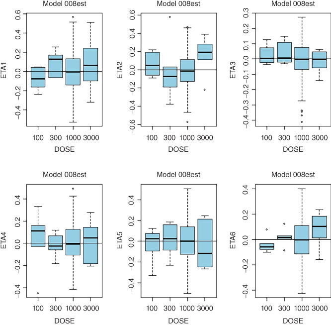
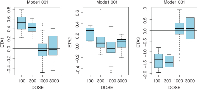
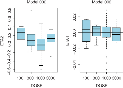
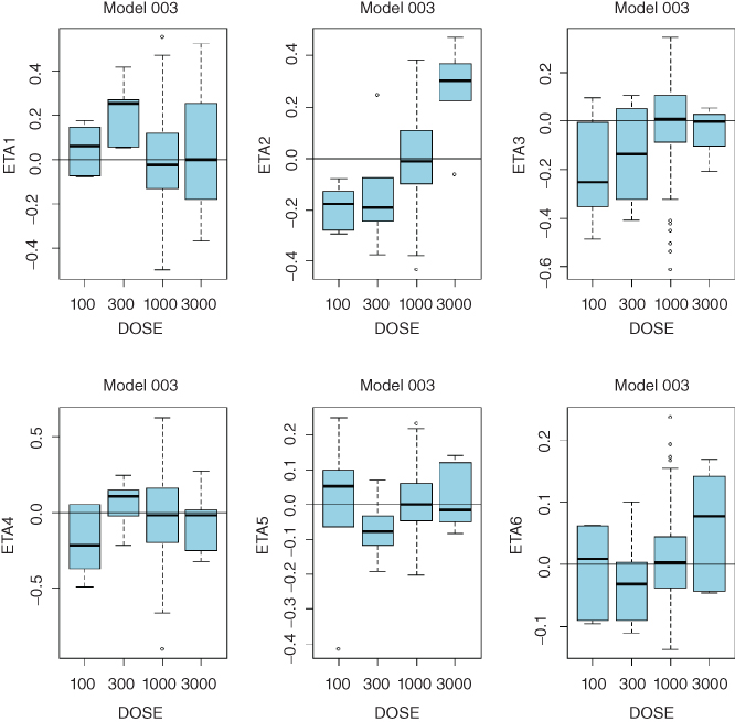
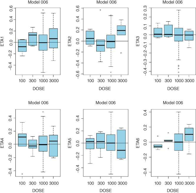
Plots of random effects vs. dose:

• Consistent trends in any of these plots may indicate that a more complex model is needed. While clearance is expected to decrease with dose in TMMD models, systematic trends for any of the model parameters may point to the need to increase complexity of the model. Sample diagnostic plots presented in the Appendix 8 illustrate incremental improvement of the model when the model complexity is increased from the linear model up to the full TMDD model. Plots for the QSS model are virtually identical to those of the full TMDD model.

Goodness of fit(GOF) plots stratified by dose:

• For nonlinear models, all GOF plots should be stratified by dose. Dose‐dependent bias in the plots of observed data versus population predictions or any other GOF plots may indicate that a more complex model is needed.

Precision of parameter estimates:

• Increase of model complexity may result in inability of the data to support estimation of all model parameters. This will be manifested in steep increase in relative standard errors (RSEs) of parameter estimates. Large RSE may indicate overparameterization and the need to go back to a simpler model structure.

Consistency of results with model assumptions and biology:

• After the model structure is selected, it is important to check whether model features are consistent with biology of the underlying system. If not, it could be hard to defend the model as the mechanistic description of the data is often the main goal of the analysis.

8.4.2 Approach Based on Biological Considerations

The alternative (or complementary) approach to model selection is based on biological considerations, i.e. on the properties of the drug and the target. The main questions to investigate are (i) whether the target is soluble or membrane‐bound; (ii) whether the internalization (elimination) rate of the drug–target complex is slow or fast; (iii) whether accumulation of the drug–target complex is small or significant relative to the total drug concentrations.

If the target is a low‐molecular‐weight, soluble molecule with a relatively fast turnover, we may expect (i) likely accumulation of the drug–target complex; (ii) availability of the free or total drug concentration measurements; (iii) availability of total target or drug–target complex concentration measurements. For these data, the QSS approximation of the TMDD model would be a model of choice.

If the target is membrane‐bound and with relatively fast turnover, we may expect (i) fast elimination of the drug–target complex; (ii) availability of only the free drug concentration measurements; (iii) low levels of total target and drug–target complex concentrations, and no measurements of these quantities. For these data, the MM approximation of the TMDD model or the model with parallel linear and MM elimination would be expected to provide an adequate description of the data.

8.5.1 Choice of ADVAN Subroutines

NONMEM versions 7.2 and 7.3 have four PREDPP subroutines (ADVAN6, ADVAN8, ADVAN9, and ADVAN13) that solve differential equations. Comparison of the performance of these routines for identical models (the QSS approximation of the TMDD model) showed that different ADVAN subroutines provided similar if not identical parameter estimates. ADVAN13 provided the fastest and most robust solution. ADVAN6 required the same or slightly longer run time, but sometimes failed even when ADVAN13 was successful. ADVAN8 and ADVAN9 were significantly less efficient. There were cases when models with ADVAN6 converged successfully or provided successful covariance step while ADVAN13 counterparts converged with rounding errors, but the opposite effects were also observed. Performance of these subroutines may depend on details of the data and stiffness of the underlying differential equations. Therefore, results may be project‐specific. We would recommend the use of ADVA13 or ADVAN6 subroutines, with switching between them as needed for a specific dataset. In NONMEM Version 7.4, two new subroutines (ADVAN14 and ADVAN15) were introduced. In our tests, performance of ADVAN14 and ADVAN15 with TMDD models was similar to that of ADVAN13 and ADVAN9, respectively.

8.5.2 Parallel Computing

The run time of TMDD models can be extremely long, especially for large data sets. Therefore, it is beneficial if not necessary to use parallel computing option provided by NONMEM. The user chooses the number of processors that is used for each problem. As NONMEM parallelization works by distribution of whole‐subject computations across processors, it makes no sense to use more processors than number of subjects in the data set. However, this is a very crude estimate as efficiency of the overall run may depend on a particular implementation of the hardware configuration, network speed, and specific details of the data. For each data set and each hardware configuration, there is a point beyond which efficiency of parallelization is greatly reduced. Moreover, the overall run time may even increase with addition of extra processors. For long‐run time problems, it is helpful to test parallel computing at the start of each project, and then use this tool appropriately. It is also beneficial to check whether NONMEM default size parameters provide sufficient memory allocation to avoid data exchange with the hard drive. It can be verified by checking that files FILE07 to FILE39 in the NONMEM run directory have size of zero. If any of these files is not empty, $SIZE option should be changed as recommended in the manual. To guarantee reproducibility of the model runs for MCMC methods independently of the computer load and number of used processors, estimation step option RANMETHOD with the descriptor P is recommended (e.g. RANMETHOD=P). This option allows NONMEM to associate the seed of the random number generator with each subject, thus allowing for the same sequence of random numbers to be used for MCMC procedures independently of parallelization options.

• Linear Model 001:
• ETA1–ETA3: random effects on CL, V_c, and Q. DOSE: nominal dose

• Model 002 with Parallel Linear and Michaelis–Menten Elimination:
• ETA1–ETA5: random effects on CL, V_c, Q, V_max, and K_SS. DOSE: nominal dose

• QSS Model 003 with Constant Target Concentration:
• ETA1–ETA5: random effects on CL, V_c, Q, K_SS, k_int, and R_tot. DOSE: nominal dose

• QSS Model 006:
• ETA1–ETA6: random effects on CL, V_c, Q, k_int, k_syn, and k_deg. DOSE: nominal dose

• Full TMDD Model 008est:
• ETA1–ETA6: random effects on CL, V_c, Q, k_int, k_syn, and k_deg. DOSE: nominal dose

References

- 1 Beal, S., Sheiner, L.B., Boeckmann, A., and Bauer, R.J. (1989–2014). NONMEM User's Guides. Ellicott City, MD: Icon Development Solutions.
- 2 Gibiansky, L., Gibiansky, E., Kakkar, T., and Ma, P. (2008). Approximations of the target‐mediated drug disposition model and identifiability of model parameters. J. Pharmacokinet. Pharmacodyn. 35 (5): 573–591.
- 3 Gibiansky, L., Gibiansky, E., and Bauer, R. (2012). Comparison of NONMEM 7.2 estimation methods and parallel processing efficiency on a target‐mediated drug disposition model. J. Pharmacokinet. Pharmacodyn. 39 (1): 17–35. https://doi.org/10.1007/s10928‐011‐9228‐y.
Appendix Diagnostic Plots