
Chapter 23
Options
The haunted house, or how to pay for being frightened!
In previous chapters, we saw that when calculating net present value, the required rate of return includes a risk premium that is added to the time value of money. The study of options is useful from a purely financial point of view, as it highlights the notion of remuneration of risk.
True, options are more complex than shares or bonds. Moreover, in their daily use they have more to do with financial management than finance. However, we will see that many financial products (warrants, stock options) can be analysed as options or as the combination of an option and a less risky asset. Have some fun by discovering the options hidden in any financial product!
A convertible bond can be seen as a combination of a conventional bond and an option. An undrawn revolving credit facility can be analysed as an option on a loan.
We will also examine how options theory can be applied to major financial strategy decisions within a company.
The purpose of this chapter is not to make you a wizard in manipulating options or to teach you the techniques of speculation or hedging with options, but merely to show you how they work in practice.
Section 23.1 Definition and theoretical foundation of options
1. Some basic definitions
There are call (buy) options and put (sell) options. The asset that can thereby be bought or sold is called the underlying asset. This can be either a financial asset (stock, bond, Treasury bond, forward contract, currency, stock index, etc.) or a physical one (a raw material or mining asset, for example).
The price at which the underlying asset can be bought or sold is called the strike price. The holder of an option may exercise it (i.e. buy the underlying asset if he holds a call option or sell it if he holds a put option) either at a given date (exercise date) or at any time during a period called the exercise period, depending on the type of option held.
A distinction is made between US-style options (the holder can exercise his right at any moment during the exercise period) and European-style options (the holder can only exercise his right on the exercise date). Most listed options are US-style options, and they are found on both sides of the Atlantic, whereas most over-the-counter (OTC) options are European-style.
Here are two examples:
Let’s say Peter sells Helmut a call option on the car manufacturer BMW having an €85 strike price and maturing in nine months. For nine months (US-style option) or after nine months (European-style option), Helmut will have the right to buy one BMW share at a price of €85, regardless of BMW’s share price at that moment. Helmut is not required to buy a share of BMW from Peter, but if Helmut wants to, Peter must sell him one for €85.
Obviously, Helmut will exercise his option only if BMW’s share price is above €85. Otherwise, if he wants to buy a BMW share, he will simply buy it on the market for less than €85.
Now let’s say that Paul buys from Clara put options on $1m in currency at an exchange rate of €1.1/$, exercisable six months from now. Paul may in six months’ time (if it’s a European-style option) sell $1m to Clara at €1.1/$, regardless of the dollar’s exchange rate at that moment. Paul is not required to sell dollars to Clara but, if he wants to, Clara must buy them from him at the agreed price.
Obviously, Paul will only exercise his option if the dollar is trading below €1.1.
The above examples highlight the fundamentally asymmetric character of an option. An option contract does not grant the same rights or obligations to each side. The buyer of any option has the right but not the obligation, whereas the seller of any option is obliged to follow through if the buyer requests.
The value at which an option is bought or sold is sometimes called the premium. It is obviously paid by the buyer to the seller, who thereby obtains some financial compensation for a situation in which he has all the obligations and no rights.
Hence, a more precise definition of an option would be:
When the option matures, we can show the payouts for the buyer and the seller of the call option in the following way:

At maturity, if BMW is trading at €90, Helmut will exercise his option and buy his BMW share at €85. He can then sell it again if he wishes, and make €5 in profit (minus the premium he paid for the option).
Similarly, for the put option:

This diagram highlights the asymmetry of risk involved: the buyer of the option risks only the premium, while his potential profit is almost unlimited, while the seller’s gain is limited, but his loss is potentially unlimited.
2. The theoretical basis of options
In a risk-free environment, if we knew today with certainty what would happen tomorrow, options would not exist as they would be completely unnecessary.
If the future were known with certainty there would be no risk and all financial assets would bring in the same return, i.e. the risk-free rate. What purpose would an option have, i.e. the right to buy or sell, if we already knew what the price would be at maturity? What purpose would a call option on Siemens serve, at a strike price of €170, if we already knew that Siemens’s share price would be below €160 at maturity and that the option would therefore not be exercised? And if we knew that, at maturity, Siemens’s share price would be €250, the price of the option would be such that it would offer the risk-free rate, just like Siemens’s shares, since the future would be known with certainty.
Options might therefore be called pure financial products, as they are merely remuneration of risk. There is no other basis to the value of an option.
Section 23.2 Mechanisms used in pricing options
Let’s suppose that Felipe buys a call option on Solvay at a €50 strike price, maturing in nine months, and simultaneously sells a put option on the same stock at a €50 strike maturing in nine months. Assuming the funds paid for the call option are largely offset by the funds received for the sale of the put option, what will happen at maturity?
If Solvay is trading at above €50, Felipe will exercise his call option and pay €50. The put option will not be exercised, as his counterparty will prefer to sell Solvay at the market price.
If Solvay is trading below €50, Felipe will not exercise his call option, but the put option that he sold will be exercised and Felipe will have to buy Solvay at €50.
Hence, regardless of the price of the underlying asset, buying a call option and selling a put option on the same underlying asset, at the same maturity and at the same strike price, is the same thing as a forward purchase of the underlying asset at maturity at the strike price.
In other words:
Assuming fairly valued markets, we can thus deduce that at the maturity of the exercise period:
It looks like this on a chart:

We can see that the profit (or loss) of this combination is indeed equal to the difference between the price of the underlying asset at maturity and the strike price.
Let’s now consider the following transaction: Evgueni wants to buy Solvay stock, but does not have the funds necessary at his immediate disposal. However, he will be receiving €50 in nine months, enough to make the purchase. He can thus borrow the present value of €50, nine months out, and buy Solvay.
At maturity, the profit (or loss) on this transaction will thus be equal to the difference between the value of the Solvay shares and the repayment of the €50 loan.
So we are back to the previous case and can thus affirm that in value terms:
This equation shows that we can “manufacture” a synthetic call option based on a put option and vice versa, as long as we can buy and sell the underlying asset and place or borrow funds.
We have used a stock for the underlying asset, but the above statement applies to any underlying asset (currencies, bonds, raw materials, etc.).
Section 23.3 Analysing options
1. Intrinsic value
Intrinsic value is the difference (if it is positive) between the price of the underlying asset and the option’s strike price. For a put option, it’s the opposite. In the rest of this chapter, unless otherwise mentioned, we will use call options as examples.
By definition, intrinsic value is never negative.
Let’s take a call option on sterling, with a strike price of €1.5/£ and maturing at end-December. Let’s say that it is now June and that the pound is trading at €1.6.
What is the option’s value? The holder of the option may buy a pound for €1.5, while the pound is currently at €1.6.
This immediate possible gain is none other than the option’s intrinsic value, which will be billed by the seller of the option to the buyer. The option will be worth at least €0.1.
Technically, a call option is said to be:
- out of the money when the price of the underlying asset is below the strike price (zero intrinsic value);
- at the money when the price of the underlying asset is equal to the strike price (zero intrinsic value);
- in the money when the price of the underlying asset is above the strike price (positive intrinsic value).
The reader will have understood that a put option is said to be:
- out of the money when the price of the underlying asset is above the strike price (zero intrinsic value);
- at the money when the price of the underlying asset is equal to the strike price (zero intrinsic value);
- in the money when the price of the underlying asset is below the strike price (positive intrinsic value).
2. Time value
Now let’s imagine that sterling is trading at €1.4 in October. The option would be out of the money (€1.4 is less than the €1.5 strike price) and the holder would not exercise it. Does this mean that the option is worthless? No, because there is still a chance, however slight, that sterling will move over €1.5 by the end of December. This would make the option worth exercising. So the option has some value, even though it is not worth exercising right now. This is called time value.
For an in-the-money option, i.e. whose strike price (€1.5) is below the value of the underlying asset (let’s now assume that £1 = €1.7), intrinsic value is €0.2. But this intrinsic value is not all of the option’s value. Indeed, we have to add time value, which ultimately is just the anticipation that intrinsic value will be higher than it is currently. For there is always a probability that the price of the underlying asset will rise, thus making it more worthwhile to wait to exercise the option.
In more concrete terms, time value represents “everything that could happen” from now until the option matures.
Hence:


Time value diminishes with the passage of time, as the closer we get to the maturity date, the less likely it is that the price of the underlying asset will exceed the strike price by that date. Time value vanishes on the date the option expires.
This means that an option is worth at least its intrinsic value, but is there an upper limit on the option’s value?
In our example, the value at maturity of the call option on sterling is as follows:
- If sterling is trading above €1.5, the option is worth the current price of sterling less €1.5, i.e. its intrinsic value, which is below the value of the underlying asset.
- If sterling is below or equal to €1.5, the option will be worthless (i.e. no intrinsic value) and therefore even further below the price of the underlying asset.
This means that if the option’s value is equal to the price of the underlying asset, then all operators will sell the option to buy the underlying asset, as their gain will be greater in any case.
Section 23.4 Parameters to value options
There are six criteria for determining the value of an option. We have already discussed one of them, the price of the underlying asset. The other five are:
- the strike price;
- the volatility of the underlying asset;
- the option’s maturity;
- the risk-free rate;
- the dividend or coupon, if the underlying asset pays one out.
1. Price of the underlying asset
As we saw earlier, all other criteria being equal, the value of a call option will be higher with a higher price of the underlying asset.
Symmetrically, the value of a put option will be lower with a higher price of the underlying asset.
2. Strike price
This is just common sense: the higher a call option’s strike price, the less chance the price of the underlying asset will exceed it. It is thus normal that the value of this call option is lower. However, the price of the put option will rise as the underlying asset can be sold at a higher price.
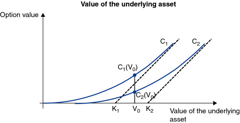
The value of a call option (call) is inversely proportional to the strike price.
3. Volatility in the value of the underlying asset
Here again, this is easy to understand: the more volatile the underlying asset, the more likely it is to rise and fall sharply. In the first case, the return will be greater for the holder of a call option; in the second case, it will be greater for the holder of a put option. As an option is nothing more than pure remuneration of risk, the greater that risk is, the greater the remuneration must be, and thus the option’s value.

Time value rises with the volatility of assets.
4. The time to maturity
You can easily see that the further away maturity is, the greater the likelihood of fluctuations in the price of the underlying asset. This raises the option’s value.

The further away maturity is, the greater time value is.
5. The risk-free rate
We have seen that the passage of time has a cost: the risk-free rate. The further away the maturity date on an option, the further away the payment of that cost. The holder of a call (put) option will thus have a cash advantage (disadvantage) that depends on the level of the risk-free rate.
The buyer of the call option pays the premium, but pays the strike price only when exercising the option. Everything happens as if he was buying on credit until “delivery”. The amount borrowed is, in fact, the present value of the strike price discounted at the risk-free rate, as we have seen previously.
Interest rates have much less influence on the value of an option than the other five factors.
6. Dividends or coupons
When the underlying asset is a stock or bond, the payment of a dividend or coupon lowers the value of the underlying asset. It thus lowers the value of a call option and raises the value of a put option. This is why some investors prefer to exercise their calls (on US-style options) before the payment of the dividend or coupon.
We can summarise the change in price of the option depending on the change in criterion in the following table:

Section 23.5 Methods for pricing options
1. Reasoning in terms of arbitrage (binomial method)
To model the value of an option, we cannot use discounting of future cash flow at the required rate of return as we have for other financial securities, because of the risk involved. Cash flow depends on whether or not the option will be exercised and the risk varies constantly. Hence, the further the option is into the money, the higher its intrinsic value and the less risky it is.
Cox et al. (1979) thus had the idea of using arbitrage logic in comparing the profit generated with options, with a direct position on the underlying asset.
Let’s take the example of a call option with a €105 strike price on a given stock (currently trading at €100) and for a given maturity.
Let’s also assume that there are only two possibilities at the end of this period: either the stock is at €90 or it is at €110. At maturity, our option will be worth its intrinsic value, i.e. either €0 or €5, or €0 or €20 if we held four options instead of just one.
We can try to obtain the same result (€0 or €20) in the same conditions using another combination of securities (a so-called replicating portfolio). If we achieve this result, the four call options and this other combination of securities should have the same value. If we can determine the value of this other combination of securities, we will have succeeded in valuing the call option.
To do so, let’s say you borrow (at 5%, for example) a sum whose value (principal and interest) will be €90 at the end of the period concerned, and then buy a share for €100 today.
At the end of the period:
- either the share is worth €110, in which case the combination of buying the share and borrowing money is worth €110 − €90 = €20; or
- the share is worth €90, in which case the replicating portfolio is worth 90 − 90 = 0.
Since the two combinations – the purchase of four call options on the one hand, and borrowing funds and buying the share directly on the other hand – produce the same cash flows, regardless of what happens to the share price, their values are identical. Otherwise, arbitrage traders would quickly intervene to re-establish the balance. So what is the original value of this combination? Let’s look at it this way: €14.3 corresponds also to the value of the four call options. We thus deduce that the call option at a €105 strike is worth €3.58. We have valued the option using arbitrage theory.
“Delta” is the number of shares that must be bought to duplicate an option. In our example, four calls produce a profit equivalent to the purchase of one share. The option’s delta is therefore 1/4, or 0.25.
Hence:
We can therefore conclude that:
Our example above obviously oversimplifies in assuming that the underlying asset can only have two values at the end of the period. However, now that we have understood the mechanism, we can go ahead and reproduce the model in backing up two periods (and not just one) before the option matures. This is called the binomial method, because there are two possible states at each step. By multiplying the number of periods or dividing each period into sub-periods, we can obtain a very large number of very small sub-periods until we have a very large number of values for the stock at the option’s maturity date, which is more realistic than the simplified schema that we developed above.
Here is what it looks like graphically:

2. The Black–Scholes model
In a now famous article, Fisher Black and Myron Scholes (1972) presented a model for pricing European-style options that is now very widely used. It is based on the construction of a portfolio composed of the underlying asset and a certain number of options such that the portfolio is insensitive to fluctuations in the price of the underlying asset. It can therefore return only the risk-free rate.
The Black–Scholes model is the continuous-time (the period approaches 0) version of the discrete-time binomial model. The model calculates the possible prices for the underlying asset at maturity, as well as their respective probabilities of occurrence, based on the fundamental assumption that this is a random variable with a log-normal distribution.
For a call option, the Black–Scholes formula is as follows:
with:

where V is the current price of the underlying asset, N(d) is a cumulative standard normal distribution (average = 0, standard deviation = 1), K is the option’s strike price, e is the exponential function, r F is the continual annual risk-free rate, s the instantaneous standard deviation of the return on the underlying asset, T the time remaining until maturity (in years) and ln the Naperian logarithm.
In practice, the instantaneous return is equal to the difference between the logarithm of the share price today and yesterday’s share price:
To cite an example: the value of a European-style nine-month call, with a strike price of €100, share price today of €90, a 3.2% risk-free rate and a 20% standard deviation of instantaneous return, is €3.3.
Comparing the model equation formula from page 415, you will see that N(d 1) is the option’s delta, while
![]() represents the present value of the strike price.
represents the present value of the strike price.
Hence:
The Black–Scholes model was initially designed for European-style stock options. The developers of the model used the following assumptions:
- no dividend payout throughout the option’s life;
- constant volatility in the underlying asset over the life of the option, as well as the interest rate;
- liquidity of the underlying asset so that it can be bought and sold continuously, with no intermediation costs;
- that market participants behave rationally!
More complex models have been derived from Black and Scholes to surmount these practical constraints. The main ones are those of Garman and Kohlhagen (1983) for currency options and Merton (1976), which reflects the impact of the payment of a coupon during the life of a European-style option.
US-style options are more difficult to analyse and depend on whether or not the underlying share pays out a dividend:
- If the share pays no dividend, then the holder of the option has no reason to exercise it before it matures. He will sell his option rather than exercise it, as exercising it will make it lose its time value. In this case, the value of the US-style call option is thus identical to the value of a European-style call option.
- If the share does pay a dividend, then the holder of the call may find it worthwhile to exercise his option the day before the dividend is paid. To determine the precise value of such an option, we have to use an iterative method requiring some calculations developed by Roll (1977). However, we can simplify for a European-style call option on an underlying share that pays a dividend: the Black–Scholes model is applied to the share price minus the discounted dividend.
The formula for valuing the put option is as follows:
Of the six criteria of an option’s value, five are “given” (price of the underlying asset, strike price, maturity date, risk-free rate and, where applicable, dividend); only one is unknown: volatility.
From a theoretical point of view, volatility would have to be constant for the Black–Scholes model to be applied with no risk of error, i.e. historical volatility (which is observed) and anticipated volatility would have to be equal. In practice, this is rarely the case: market operators adjust upward and downward the historical volatility that they calculated (over 20 days, one month, six months, etc.) to reflect their anticipation of the future stability or instability of the underlying asset. However, several classes of options (same underlying, different maturity or strike price) can be listed for the same underlying asset. This allows us to observe the implied volatility of their quoted prices and thus value the options of another class.
This is how anticipated volatility is obtained and is used to value options. This practice is so entrenched that options market traders trade anticipation of volatility directly.
Anticipated volatility is then applied to models to calculate the value of the premium.
The Black–Scholes model can thus be used “backwards”, i.e. by taking the option’s market price as a given and calculating implied volatility. The operator can then price options by tweaking the price on the basis of his own anticipation. He buys options whose volatility looks too low and sells those whose implied volatility looks too high.
It is interesting to note that, despite these simplifying assumptions, the Black–Scholes model has been de facto adopted by market operators, each of them adapting it to the underlying asset concerned.
Section 23.6 Tools for managing an options position
Managing a portfolio of options (which can also be composed of underlying assets or the risk-free asset) requires some knowledge of four parameters of sensitivity that help us measure precisely the risks assumed and develop speculative, hedging and arbitrage strategies.
1. The impact of fluctuations in the underlying asset: delta and gamma
We have already discussed the delta, which measures the sensitivity of an option’s value to fluctuations in the value of the underlying asset. For calls and puts that are significantly out of the money, the value of the option may not change much when the underlying asset moves up or down. As the price of the underlying asset moves to a level substantially above the strike for calls or below the strike for puts, the option becomes more valuable and more sensitive to changes in the underlying asset.
Mathematically, the delta is derived from the option’s theoretical value vis-à-vis the price of the underlying asset and is thus always between 0 and 1, either positive or negative. Whether it is positive or negative depends on the type of option.
We have seen that, when using the Black–Scholes formula, the delta of a call option is equal to N(d 1). The delta of a put option is equal to N(d 1) − 1. This relationship is prized by managers of options portfolios, as it links the option’s value and the value of the underlying asset directly. Indeed, we have seen that the delta is, above all, an underlying equivalent: a delta of 0.25 tells us that a share is equivalent to 4 options. But above all, managers use the delta as an indicator of sensitivity: how much does the option’s value vary in euros when the underlying asset varies by one euro?
The delta of a call option that is far in-the-money is very close to 1, as any variation in the underlying asset will show up directly in the option’s value, which is essentially made up of intrinsic value.
Similarly, a call option that is far out-of-the-money is composed solely of its time value and a variation in the underlying asset has little influence on its value. Its delta is thus close to 0.
The delta of an at-the-money call option is close to 0.5, indicating that the option has as much chance as not of being exercised.
This is expressed in the following table:
| Out-of-the-money | At-the-money | In-the-money | |
| Call option | 0 < delta < 0.5 | delta = 0.5 | 0.5 < delta < 1 |
| Put option | −0.5 < delta < 0 | delta = −0.5 | −1 < delta < −0.5 |
The delta can also express probability of expiration in-the-money for options close to maturity and whose underlying asset is not too volatile: a delta of 0.80 means that there is an 80% probability that the option will expire in-the-money.
Unfortunately, the delta itself varies with fluctuations in the underlying asset and with the passing of time. Changes in the delta of an option create either a risk or an opportunity for investors and traders. Hence, the idea of measuring the sensitivity of delta to variations in the value of the underlying asset: this is what gamma does. Mathematically, it is none other than a derivative of the delta vis-à-vis the underlying asset, and is often called the delta of the delta!
The gamma of an option is largest near the strike price. A zero-gamma options position is completely immune to fluctuations in the value of the underlying asset.
2. The impact of time: theta
Options are like people: they run down with time. Even if there is no change in the underlying asset price, the passage of time alone shows up in gains or losses for the option’s holder.
Mathematically speaking, the theta is equal to the opposite of the derivative of the theoretical value of the option with respect to time. Theta measures how much an option loses in value if no other factors change.
3. The impact of volatility: vega
Vega is the rate of change in the derivative of the theoretical value of the option vis-à-vis implied volatility. Vega is always positive for a call option, as for a put option, as we have seen that the time value of an option is an increasing function of volatility.
All other factors being equal, the closer an option is to being in the money (with maximum time value), the greater the impact of an increase in volatility.
While each of the tools presented here is highly useful in and of itself, combining them tells us even more. In practice, it is impossible to create a position that is neutral on all criteria at once. No return is possible when taking no risk. No pain, no gain! Hence, a delta-neutral position and a gamma-negative position must necessarily have a positive theta in order to be profitable.
4. Implied volatility
From 1990, the CBOE (Chicago Board Options Exchange) has calculated the VIX, an index of the implied volatility of the Standard & Poor’s 100, using at-the-money options with a maturity shorter than one month. The options on the S&P 100 are sufficiently liquid to consider this index representative of the implied volatility on the market.
The following graph shows the evolution of VIX from its initial launch.

If returns actually followed a Gaussian distribution, the Dow Jones would change daily by more than 7% only once in 300 000 years. In the 20th century there were 48 such changes, and there have been two since 2000. Recent studies have shown that the distribution of return has a configuration something like this.
Source: Bloomberg & Datastream (CBOE Volatility Index on S&P100 until 31/12/2006 and S&P500 since)
5. Model risk
Options markets, whether organised (listed) or not (over-the-counter), have developed considerably since the mid-1970s, as a result of the need for hedging (of currency risks, interest rates, share prices, etc.), an appetite for speculation (an option allows its holder to take a position without having to advance big sums) and the increase in arbitrage trading.
In these conditions, a new type of approach to risk has developed on trading floors: model risk. The notion of model risk arose when some researchers noticed that the Black–Scholes model was biased, since (like many other models) it models share prices on the basis of a log-normal distribution. We have seen empirically that this type of distribution significantly minimises the impact of extreme price swings.

This has given rise to the notion of model risk, as almost all banks use the Black–Scholes model (or a model derived from it). Financial research has uncovered risks that had hitherto been ignored.
An anomaly in the options market highlights the problems of the Black–Scholes model. When we determine the implied volatility of an underlying asset (the only factor not likely to be observed directly) based on the price of various options having the same underlying asset, we can see that we do not find a single figure. Hence, the implied volatility on options far out-of-the-money or far in-the-money is higher than the implied volatility recalculated on the basis of at-the-money options. This phenomenon is called the volatility smile (because when we draw volatility on a chart as a function of strike price, it looks like a smile).
We will see in the following chapters the many applications of options in corporate finance:
- to raise financing (see Chapter 25);
- to resolve conflicts between management and ownership or between ownership and lenders (see Chapter 34);
- to hedge risks and invest (see Chapter 50);
- to choose investments (see Chapter 30);
- to value assets (see Chapter 31);
- to value the equity of a company (see Chapter 34);
- to take over a company (see Chapter 44).
This gives you an idea of the importance of options.