Does paradise exist in the world of finance?

The central question of this chapter (and of the following one) is: is there an optimal capital structure? That is to say, is there a “right” combination of equity and debt that allows us to reduce the weighted average cost of capital and therefore to maximise the value of capital employed (enterprise value)?

The reader may be surprised by this question when Chapter 13 showed clearly how return on equity could benefit from the leverage effect. But again we recall that we have now left the world of accounting in order to enter the universe of finance.

Jumping directly to the conclusion, this part of the book could be renamed “the uselessness of the leverage effect in finance”!

Note that we consider the weighted average cost of capital (or cost of capital), denoted k, to be the rate of return required by all the company’s investors either to buy or to hold its securities. It is the company’s cost of financing and the minimum return its investments must generate in the medium term. If not, the company is heading for ruin.

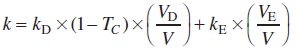
k _D is the rate of return required by the lenders of a given company, k _E is the cost of equity required by the company’s shareholders, and k is the weighted average rate of the two types of financing, equity and net debt (from now on often referred to simply as debt). The weighting reflects the breakdown of equity and debt in enterprise value.

With V _D the market value of net debt and V _E the market value of equity, we get:

or, since the enterprise value is equal to the value of net debt plus equity (EV = V = 
V _E + V _D):

If, for example, the rate of return required by the company’s creditors is 6%, the corporate tax rate is 33%, the rate of return required by the shareholders is 10% and the value of debt is equal to that of equity, then the return required by all of the company’s sources of funding will be 7%.¹ Its weighted average cost of capital is thus 7%.

To simplify our calculations and demonstrations in this chapter, we shall assume infinite durations for all debt and investments. This enables us to apply perpetual bond analytics and to assume that the company’s capital structure remains unchanged during the life of the project, income being distributed in full. The assumption of an infinite horizon is just a convention designed to simplify our calculations and demonstrations, but they remain accurate within a limited time horizon (say, for simplicity, 15–20 years).

Section 32.1 The value of capital employed

While accounting looks at a company by examining its past and focusing on its costs, finance is mainly a projection of the company into the future. Finance reflects not only risk but also – and above all – the value that results from the perception of risk and future returns.

From now on, we will speak constantly of value. As we saw previously, by value we mean the present value of future cash flows discounted at the rate of return required by investors:

• equity (E) will be replaced by the value of equity (V _E);
• net debt (D) will be replaced by the value of net debt (V _D);
• capital employed (CE) will be replaced by enterprise value (EV), or firm value.

We will speak in terms of a financial assessment of the company (rather than the accounting assessment provided by the balance sheet). Our financial assessment will include only the market values of assets and liabilities:

As operating assets are financed by equity and net debt (which are accounting concepts), logically, a company’s enterprise value will consist of the market value of net debt and the market value of equity (which are financial concepts). This chapter therefore reasons in terms of:

Important: Enterprise value is sometimes confused with equity value. Equity value is the enterprise value remaining for shareholders after creditors have been paid. To avoid confusion, remember that enterprise value is the sum of equity value and net debt value.

Similarly, we will reason not in terms of return on equity, but rather required rate of return, which was discussed in depth in Chapter 19. In other words, the accounting notions of ROCE (return on capital employed), ROE (return on equity) and i (cost of debt), which are based on past observations, will give way to WACC or k (required rate of return on capital employed), k _E (required rate of return on equity) and k _D (required rate of return on net debt), which are the returns required by those investors who are financing the company.

Section 32.2 Debt and equity

The fundamental differences between debt and equity should now be crystal clear.

• Debt:
  • provides a return for the investor that is independent of the performance of the firm. Except in extreme cases (default, bankruptcy), the lender will earn the interest due (no more, no less) regardless of whether the earnings of the company are excellent, average or bad;
  • always has a term, even if remote in time, that is defined contractually. We will not consider for the time being the rare cases of perpetual debts (which are usually only named so when you analyse them more carefully);
  • is repaid in priority to equity in case of liquidation of the company – the proceeds of the sale of assets will primarily go to lenders, and only if and when lenders have been fully repaid will shareholders receive cash.
• Equity:
  • yields returns depending on the profitability of the company. Dividends and capital gains will be nil if the results are not good on a long-term basis;
  • does not benefit from a repayment commitment. The only exit for equity can be found by selling to a new shareholder, which will take over the role from the previous one;
  • in case of bankruptcy is repaid only after all creditors have been fully repaid. Our readers probably know that in most cases the proceeds from liquidation are not sufficient to repay 100% of creditors. Shareholders are then left with nothing as the company is insolvent.

Shareholders fully run the risk of the firm as the cash flows generated by the capital employed (free cash flows to the firm) will first be allocated to lenders; only when they have collected what is due will shareholders be entitled to the remainder.

Given these elements, it becomes natural that the voting rights and therefore the right to choose management lies in the hands of shareholders. Shareholders have a vested interest that capital employed be managed in an optimal manner by management, so that it generates high cash flows after the service of debt (interest and capital repayments).

Voting rights do not really represent a fourth difference between equity and debt and are only a logical consequence of the first three differences. It is only because shareholders are second to lenders in the collection of cash flows generated by the capital employed, hence running the risk of the firm, that they benefit from voting rights.

The higher the enterprise value, the higher also the equity value. As debt does not run the risk of the firm (except in case of financial distress), its value will largely be independent of the changes in enterprise value. We find here again the concept of leverage, as a small change in enterprise value can have a large impact on equity value.

It should be noted that these two graphs are not on the same scale (the first one on annual cash flows, the second one on values).

Section 32.3 What our grandparents thought

We shall start by assuming a tax-free environment, both for the company and the investor, in which neither income nor capital gains are taxed. In other words, heaven! Concretely, the optimal capital structure is one that minimises k, i.e. that maximises the enterprise value (V). Remember that the enterprise value results from discounting free cash flow at rate k. However, free cash flow is not related to the type of financing. The demonstrations below endeavour to measure and explain changes in k according to the company’s capital structure.

We know that ex-ante debt is always cheaper than equity (k _D < k _E) because it is less risky. Consequently, a moderate increase in debt will help reduce k, since a more expensive resource (equity) is being replaced by a cheaper one (debt). This is the practical application of the preceding formula and the use of leverage.

However, any increase in debt also increases the risk for the shareholder. Markets then demand a higher k _E, the more debt we add in the capital structure. The increase in the expected rate of return on equity cancels out part (or all, if the firm becomes highly leveraged!) of the decrease in cost arising on the recourse to debt. More specifically, the traditional theory claims that a certain level of debt gives rise to a very real risk of bankruptcy. Rather than remaining constant, shareholders’ perception of risk evolves in stages.

The risk accruing to shareholders increases in step with that of debt, prompting the market to demand a higher return on equity. This process continues until it has cancelled out the positive impact of the debt financing.

At this level of financial leverage the company has achieved the optimal capital structure, ensuring the lowest weighted average cost of capital and thus the highest enterprise value. Should the company continue to take on debt, the resulting gains would no longer offset the higher return required by the market.

Moreover, the cost of debt increases after a certain level because it becomes more risky. At this point, not only has the company’s cost of equity increased, but also that of its debt.

In short, the evidence from the “real world” shows that an optimal capital structure can be achieved with some – but not too much – leverage.

In this example, the debt-to-equity ratio that minimises k is 0.4. The optimal capital structure is thus achieved with 40% debt financing and 60% equity financing.

Section 32.4 The capital structure policy in perfect financial markets

We shall demonstrate this proposition by means of an example given by Franco Modigliani 
and Merton Miller (MM), who showed that, in a perfect market and without taxes, the traditional approach is wrong. If there is no optimal capital structure, then the overall cost of equity ( k or WACC) remains the same regardless of the firm’s debt policy.

The main assumptions behind the theorem are:

1. companies can issue only two types of securities: risk-free debt and equity;
2. financial markets are frictionless;
3. there is no corporate and personal taxation;
4. there are no transaction costs;
5. firms cannot go bankrupt;
6. insiders and outsiders have the same set of information.

According to MM, investors can take on debt just like companies. So, in a perfect market, they have no reason to pay companies to do something they can handle themselves at no cost.

Imagine two companies that are completely identical except for their capital structure. The value of their respective debt and equity differs, but the sum of both, i.e. the enterprise value of each company, is the same. If the reverse were true, equilibrium would be restored by arbitrage.

We shall demonstrate this using the examples of Companies X and Y, which are identical except that X is unlevered and Y carries debt of 80 000 at 5%. If the traditional approach were correct, Y’s weighted average cost of capital would be lower than that of X and its enterprise value higher:

	Company X	Company Y
Operating profit: EBIT	20 000	20 000
Interest expense (at 5%): IE	0	4 000
Net profit: NP	20 000	16 000
Dividend: DIV = NP2	20 000	16 000
Cost of equity: k E	10%	12%
Equity: V E = DIV/k	200 000	133 333
	0	80 000
Enterprise value: V = V E + V D	200 000	213 333
Weighted average cost of capital: k = EBIT/V3	10%	9.4%
Gearing: V D/V E	0%	60%

Y’s cost of equity is higher than that of X, since Y’s shareholders bear both the operating risk and that of the capital structure (debt), whereas X’s shareholders incur only the same operating risk. As a matter of fact, the operating risk of X is the same as that of Y, as X and Y are identical but for their capital structures.

Modigliani and Miller demonstrated that Y’s shareholders can achieve a higher return on their investment by buying shares of X, at no greater risk.

Thus, if a shareholder holding 1% of Y shares (equal to 1333) wants to obtain a better return on his investment, he must:

• sell his Y shares …
• … replicate Y’s debt/equity structure in proportion to his 1% stake; that is, borrow 1333 × 60% = 800 at 5% …
• … invest all this (800 + 1333 = 2133) in X shares.

The shareholder’s risk exposure is the same as before the operation: he is still exposed to operating risk, which is the same on X and Y, as well as to financial risk, since his exposure to Y’s debt has been transferred to his personal borrowing. However, the personal wealth invested by our shareholder is still the same (1333).

Formerly, the investor received annual dividends of 160 from Company Y (12% × 1333 or 1% of 16 000). Now, his net income on the same investment will be:

He is now earning 173 every year instead of the former 160, on the same personal amount invested and with the same level of risk.

Y’s shareholders will thus sell their Y shares to invest in X shares, reducing the value of Y’s equity and increasing that of X. This arbitrage will cease as soon as the enterprise values of the two companies come into line again.

In their article, Modigliani and Miller assumed that the cost of debt would remain constant as bankruptcy was not an option. In this context, how is it possible to obtain a constant k if k_D is constant too and thus if we increase the leverage we would expect a continuously decreasing k? The answer is simple: as leverage increases, risk for shareholders increases too and they require a higher cost of equity. The increased leverage is counterbalanced by the increase in cost of equity.

We can easily erase the assumption of no distress cost. In this case, Modigliani and Miller’s proposition still stands: enterprise value does not depend on capital structure.

In this context, cost of debt (k_D) actually increases with leverage, as debtholders suffer an increasing risk of bankruptcy. Cost of equity obviously still increases with a higher level of debt, but not as fast as in Modigliani and Miller’s proposition, as shareholders are passing on part of the risk to debtholders.

Investing in a leveraged company is neither more expensive nor cheaper than investing in a company without debt; in other words, the investor should not pay twice, first when buying shares at enterprise value and then to reimburse the debt. The value of the debt is deducted from the value of the capital employed to obtain the price paid for the equity.

While obvious, this principle is frequently forgotten. And yet it should be easy to remember: the value of an asset, be it a factory, a painting, a subsidiary or a house, is the same regardless of whether it was financed by debt, equity or a combination of the two. As Merton Miller explained when receiving the Nobel Prize for Economics, “it is the size of the pizza that matters, not how many slices it is cut up into”. Or, to restate this: the weighted average cost of capital does not depend on the sources of financing. True, it is the weighted average of the rates of return required by the various providers of funds, but this average is independent of its different components, which adjust to any changes in the financial structure.

Summary

Answers

Bibliography