11.1 INTRODUCTION
In Chapter 7 we presented an approach to derive the term structure of available funding (TSFu) given the funding sources and liquidity buffer needed to cope with gap risk on rollover dates. In this chapter we design a consistent framework to build the funding (interest rate) curve of a bank, as a mix of the costs of different funding sources entering the TSFu, and we indicate a methodology on how to properly include risks related to refunding activity in the cost of funds transferred from the treasury department to business units to buy assets.
To this end, we first introduce a brief overview of fund transfer pricing (FTP) principles, then we sketch a stylized bank's balance sheet, so that in a single-period setting we can clearly disentangle the several cost and risk components entering the fair pricing of assets, such as loans. We show the single building blocks that make up the price of an asset, including market, credit and liquidity costs (along the lines sketched in Chapter 10). We focus on a theoretical framework to quantify funding costs and gauge funding risk. Finally, we show how to apply the framework in practice.
11.2 PRINCIPLES OF TRANSFER PRICING
When a bank wants to invest in a given asset, it has to calculate its value. We showed in Chapter 10 a general approach to identify funding costs as well as the profit the bank can expect to make (on a risk-adjusted basis). We now expand the analysis by considering a more complex structure of funding sources and by including unexpected costs of market and credit risk as well. We present here a simplified single-period framework to introduce the basic principles of transfer pricing.
11.2.1 Balance sheet
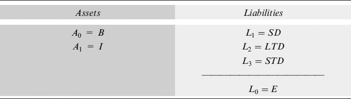
Assume that we are at time t = 0 and that the bank will end all activities in one year. The bank's balance sheet is shown in Table 11.1.
There are two assets, A0 and A1: A0 is a risk-free bond B yielding i0 = r and A1 is an investment I yielding i1 (e.g., a loan). On the liabilities' side there is equity and another three kinds of liability L1, L2, L3 (e.g., long-term and short-term debt), each one yielding, respectively, interest lj = r + sj, for j = 1,…, 3; additionally, there is equity, indicated by L0.
The share of equity L0 = E (capital allocation) invested in the risk-free investment A0 = B, is 1 − ε, whereas share ε is invested in the other asset A1. The return on capital required by stockholders is e: this is the rate at which the capital invested in the bank's activity is expected to be remunerated.
Table 11.1. Bank's stylized balance sheet
Considering the participation of equity in funding the investment, the following constraints hold:
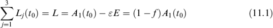
where ![]() is the fraction of the asset financed by capital, and
is the fraction of the asset financed by capital, and
11.2.2 Bank's profits and losses
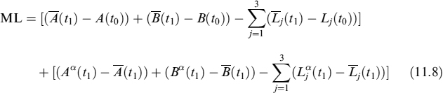
At the end of the year the assets will be sold back and they produce total profits/losses:

where we used the constraint in (11.2).
As for liabilities, they will be bought back (minus equity) at the end of the year and they generate total profits/losses:
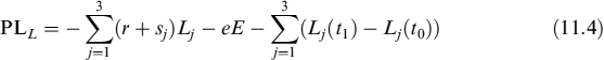
The addend (A1(t0) − A1(t1)) in (11.3) can be positive or negative: losses in the investment can be due to possible default of the bank's obligor (or more generally, bank's counterparty). Assuming that PD is the probability of default of the obligor and that ![]() is the stochastic loss suffered by the bank, we have that credit losses can be written as:
is the stochastic loss suffered by the bank, we have that credit losses can be written as:
where ![]() is the average (expected) LGD (i.e., LGD × PD),
is the average (expected) LGD (i.e., LGD × PD), ![]() is the maximum LGD, calculated at some degree of confidence according to some credit model and CVARA1 is the credit VaR (i.e., unexpected loss). We can alternatively write equation (11.5) as
is the maximum LGD, calculated at some degree of confidence according to some credit model and CVARA1 is the credit VaR (i.e., unexpected loss). We can alternatively write equation (11.5) as
Average credit loss ![]() (which is CVA in a loan)1 is a productive risk2 and should be compensated by spread sA1, applied to the notional A1, determined as:
(which is CVA in a loan)1 is a productive risk2 and should be compensated by spread sA1, applied to the notional A1, determined as:
where LGD is the percentage loss upon default and we assume that interest is fully recovered. Unexpected credit loss (or credit VaR) is covered by economic capital, or fraction ϕ of the equity, since typically no credit instrument is available in the market to hedge this risk.3
The other possible variations included in (A1(t0) − A1 (t1)), and in the addends (B(t1) − B(t0)) (in equation (11.3)) and ![]() (in equation (11.4)), represent profits/losses due to changes in the market value of assets and liabilities from the start t0 to the end of the year t1:4
(in equation (11.4)), represent profits/losses due to changes in the market value of assets and liabilities from the start t0 to the end of the year t1:4
where ![]() ,
, ![]() and
and ![]() are expected values at t1 for the risky asset, risk-free investment and liability j, whereas Aα(t1), Bα(t1) and
are expected values at t1 for the risky asset, risk-free investment and liability j, whereas Aα(t1), Bα(t1) and ![]() are the values for the same variables computed at confidence level α. Expected market loss is indicated by
are the values for the same variables computed at confidence level α. Expected market loss is indicated by ![]()
![]() and unexpected market loss (i.e., market VaR) by
and unexpected market loss (i.e., market VaR) by ![]()
![]() . Equation (11.8) can be rewritten as:
. Equation (11.8) can be rewritten as:
We focus on market losses (and disregard possible profits) just to stress the fact that they originate from passive risks that should be fully hedged, via traded market instruments such as swaps or FRAs, when possible. When this is not possible, unexpected losses have to be taken into account and included in the MVAR, which implies allocation of economic capital to cover it.
- Changes in risk-free interest rates: Expected change is captured by the slope of the risk-free interest rate term structure; it is a passive risk that can be hedged with market instruments, so it produces no MVAR.
- Changes in financial options embedded in the contracts (e.g., call option on the asset bought by the bank, or caps and floors for assets paying a floating rate): Expected profit/loss can be valued by the price of these options traded in the market, which can be used to hedge this passive risk, which, as such, does not generate any MVAR.
- Changes in the value of liquidity and behavioural options (e.g., prepayment option bought by the mortgagee): Expected cost can be valued using statistical and financial techniques,5 but typically a hedge with market instruments is not possible. As such, these losses are in most cases originated by productive risk and an MVAR has to be computed and taken into account when measuring the PL of an investment.
- Changes in the level of the funding spread of the bank: Expected and unexpected market losses related to refunding risk for the rollover of liabilities cannot be hedged (as demonstrated in Chapter 10): the risk is not passive, but productive since it is strictly inherent to banking activity and as such it should be included in valuation of an investment by considering the economic capital needed to cover the corresponding MVAR as well.
In theory, almost all market risks are passive since they can be hedged, so that unexpected losses are not included in the MVAR; expected losses are considered because they also represent the price of setting up hedges in the market. Besides the losses generated by interest rate risk, which enter in the valuation process directly through the interest flows related to assets and liabilities, all other losses due to financial options are collectively indicated by FO, whereas liquidity/behavioural options are indicated by LO.
Losses originated by productive market risks, such as refunding risk and some behavioural risks,6 are included in the MVAR since they cannot be hedged because either it is impossible or no hedging instrument is traded in the market.
There is also another productive risk that we analysed in Chapter 7 and that relates to the rollover of liabilities: this is funding gap risk, which is covered by a suitable amount of liquidity buffer. Maintenance of the LB causes costs that the bank has to pay and since they also include its funding spread, they cannot be hedged with market instruments. Hence, for liquidity buffer costs (LBC) too, the bank needs to calculate unexpected costs, to include them in the MVAR and to post a suitable amount of economic capital to cover them.
The CVAR and the MVAR absorb a fraction ϕ of equity: this is the economic capital required to run the banking activity and to face related productive risks. We assume, in our simplified balance sheet, that equity E is exactly the amount needed to cover unexpected market and credit loss, with no extra capital available, so ϕ = 1 and:
E = CVARA1 + MVAR
Total profits/losses are determined simply by summing up all the terms relating to assets and liabilities in equations (11.6) and (11.8):
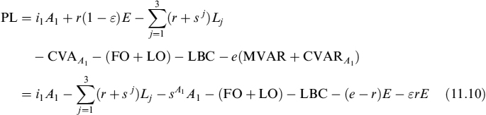
We indicate by π = (e − r) the risk premium over the risk-free rate demanded by equity holders, so that:

It is now possible to determine rate ![]() that investment A1 has to yield to break even (PL = 0):
that investment A1 has to yield to break even (PL = 0):

where ![]() is the average funding spread paid on all liabilities. Breakeven rate
is the average funding spread paid on all liabilities. Breakeven rate ![]() comprises the following components:
comprises the following components:
- ir: the risk-free rate used in the total funding cost to pay on liabilities;
- fu: funding costs due to spreads paid over the risk-free rate on liabilities;
- cl: costs relating to contingent liquidity (i.e., to the liquidity buffer that has to be kept to cope with funding gap risk);
- cs: credit spread or remuneration for expected losses in the event of default of the obligor of asset A1;
- op: the cost of financial and liquidity/behavioural options;
- cc: the cost of economic capital required to cover unexpected credit and market risks.
The breakeven, or fair, rate that includes all the components above covers all the costs related to the banking activity to invest in A1. It should be noted that in most cases, when A1 is a typical bank contract such as a loan or a mortgage, the investment can actually be considered as a product to sell to a customer. The difference between standard goods or services and a bank product is that the latter appears on a bank's balance sheet as an asset or a liability, or off balance sheet as a commitment, after it is sold. So the breakeven rate is the amount to charge the counterparty to recoup all the production costs of a product that eventually will be included on the bank's balance sheet.
The bank may also charge a margin on top of all the components we have shown to achieve a profit. This profit is remuneration to the shareholders for the equity invested in the bank: if all the investments are properly priced, remuneration is already included in the economic capital absorbed to cover related unexpected costs. This means that remuneration for the equity is already theoretically included in the valuation process in the cc component, so that any profit margin would mean double counting. In practice, it is possible that an extra margin is added: this includes the commercial margin, which is remuneration for business units selling products to clients, and the margin to cover infrastructure and, broadly speaking, other nonfinancial costs. In Figure 11.1 we schematically recapitulate the building blocks of fund transfer pricing.
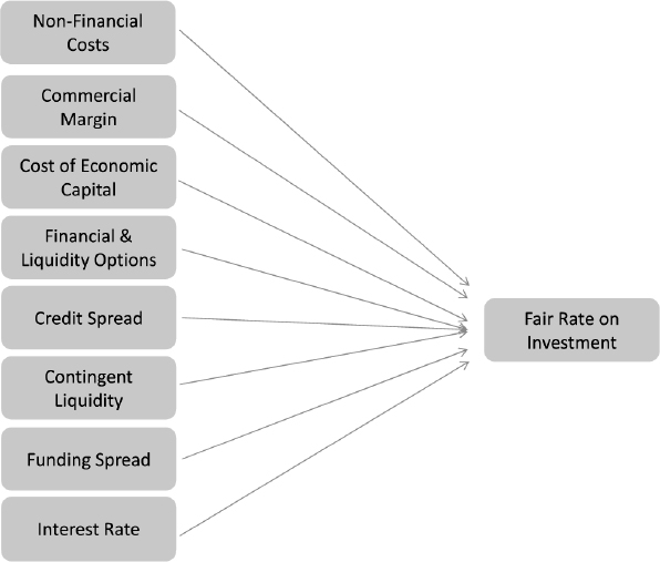
Figure 11.1. The building blocks to determine the fund transfer price of an investment
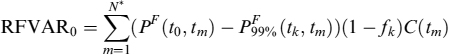
The approach we have sketched to set fund transfer prices can be defined as full-risk pricing and also serves the purpose of measuring the risk-adjusted return of the bank's investments. In fact, the PL can also be seen in value-added VA terms: recall that economic capital EC is, in our simplified world, equal to equity (E = EC = CVAR + MVAR); moreover, let us indicate by
the actual profits/losses brought about by business activity. We have
which is the definition of value added. The risk-adjusted return on capital RAROC is defined as:
If RAROC = (π + εr) (i.e., exactly equal to the required remuneration for the equity capital employed to cover unexpected losses), then VA = 0.
Both VA and RAROC can be used as ex ante measures of profitability (which is basically what we have shown above) and as ex post measures to verify whether realized profits are satisfactory for the risks taken at inception of the contract.
In what follows we will focus on the interest rate and funding spread components of FTP. A tool that properly accounts for funding is the funding curve: it indicates expected and unexpected costs of the liquidity needed to fund an investment. We will first make a detour to explain the ideas underpinning the approach we propose, then we will come back to analysis of the funding curve.
11.3 FUNDING AND BANKING ACTIVITY
Funding costs and funding transfer rates have been examined in the past, and generally the analysis (often implicitly) assumed that: (i) the financial institution was able to finance its credit intermediation activity at lower rates than those earned on activities, thus generating interest margin profits (and implying the bank's creditworthiness rather than the client's); (ii) (partly) financing short-term activities with long-term maturities was not a risky activity in practice; (iii) liquidity in the market was abundant so that choice of the funding mix was determined with almost no constraints.
The turbulence in the financial markets, starting in 2007 and becoming severer in 2008 (see Chapter 1), made these assumptions either unrealistic or at least necessitous of further refinements. First, it is no longer true that financial institutions are always able to raise funds under less expensive conditions than their clients, at least in markets where bargaining power is evenly distributed between participants, such as in the capital market. Second, the volatility of banks' funding spreads over risk-free market rates dramatically increased, so that financing long-term activities with short-term debt, even partially, is riskier than in the past and the risk has to be properly taken into account. Third, as a consequence of the first two points, the funding mix is subject to constraints that abate the average funding cost and make credit intermediation activity still profitable, while keeping the liquidity gap risk under control (see Chapter 7 for a discussion on this point).
Financial institutions realized their activity would become in some cases unprofitable if they continued using past schemes. As a very simplified example, long-term loans were often priced by considering the marginal cost for the bank on the corresponding expiry as the funding cost, which had to be added to other costs so as to set a fair loan rate. On longer expiries the only available funding source is, typically, the issuance of bonds in the capital market. Currently, such an approach would reject a large, or nonnegligible in any case, part of possible investments, depending on general market and bank-specific conditions, since bonds are usually the most expensive source of funding for a bank. Additionally, it should be noted that for really long-term contracts (say, 20-year expiry) the bank has no available source for perfectly matched funding,7 so in any case it has to make some assumptions about future evolution of the funding spread and on the rollover of liabilities.
By the very fact that banks are still doing business, they clearly have been looking at financing activity from a different perspective using new criteria along the lines we now suggest.
First, we suggest that funding cost has to take into account all possible funding sources available: regarding some of them, such as demand and saving deposits, the bank's bargaining power is relatively strong and funding cost can be significantly abated. Regarding others, such as wholesale funding, the bargaining power between counterparties is pretty even and the bank can expect to pay a fair funding spread.
Second, we believe funding mix has to be considered from a dynamic rather than static perspective: this makes possible the building of funding curves that account for (expected) average funding costs on short-term liabilities that will roll over on expiry, by assuming continuity of banking activity.8
Third, the risk inherent in liability rollover (which we term refunding risk) has to be consistently measured and accounted for so as to allocate an amount of economic capital and include it in investment pricing in a correct way. The risk we are dealing with here is twofold: on the one hand, the bank can face the problem of not being able to roll over maturing liabilities for the entire amount: this would produce gap risk and then generate the need for a liquidity buffer (we have extensively analysed this in Chapter 7). On the other hand, the bank may be able to roll over maturing liabilities fully, but only by paying a funding cost higher than expected: this is the refunding risk we have to investigate to find out how to measure and manage it. Unfortunately, this type of risk cannot be hedged, so the only way to cope with it is to set aside an adequate amount of capital in the same fashion the bank does for other productive risks.
What we propose in the following is an approach that complies with these criteria. Schematically, it can be sketched as follows:
- A funding curve for each available source has to be built up to a given expiry, generally longer than the source's average duration, by projecting future costs based on market risk-free forward rates plus the source's specific spreads over them.
- A weighted average funding curve is then calculated to determine the average (expected) cost borne by the bank to finance a given investment.
- Unexpected funding costs, due to the uncertainty relating to liability rollover, are measured by a VaR-like methodology, thus identifying unexpected maximum cost at a given level of confidence for any expiry.
- Unexpected costs imply that a given amount of economic capital has to be allocated and its remuneration has to be included in the pricing of the bank's investments.
11.4 BUILDING A FUNDING CURVE
Let us assume we have different funding sources such as demand deposits, term deposits, bonds issued in the market, etc. Let J be the number of these sources each of which entails a cost for the bank that is a function of the risk-free interest rate curve and the bank's funding spread.
Let L be, as before, the total of amount raised from different funding sources (i.e., liabilities) and define the weights wj = Lj/L, for j = 1,…, J.
Remark 11.4.1. In this chapter we do not analsye how to set the weights associated with each funding source, we simply take them as given. In Chapter 7 we outlined an approach to determine the weights based on an equilibrium criterion related to funding gap risk. If the bank adopts this approach, the weights will be time dependent. In the subsequent analysis we only consider constant weights but, as will be manifest, the extension to time-dependent weights is straightforward.
Define the discount curve Pj = {Pj(0, t1),…, Pj(0, tN)} as the collection of discount factors that can be bootstrapped from prices of the j-th funding source. We assume that it is possible to infer discount factors up to expiry tN equal for all funding sources via risk-free rates and the spread over these, which can reasonably be forecast or even implied from market prices. It is reasonable to assume that the OIS (or Eonia for the euro) rates are the best proxy for risk-free rates, so it is relatively easy to infer them from quoted swap rates. We also define the risk-free discount curve up to maturity tN, derived from interbank quotes, as PD = {PD(0, t1)…, PD(0, tN)}.
We do not go into details on how to bootstrap risk-free discount curves from the market prices of deposits, FRAs, swaps and OIS (or Eonia): we take them as given. More specifically, we assume they can be exactly generated by the CIR model with a given set of parameters.9 We know that in this model the term structure of interest rates is driven by one stochastic factor, the instantaneous interest rate rt, whose dynamics are:
The discount factors generated by the CIR model can be computed in closed form by equation (8.27).
To make things concrete, we go on to describe the theoretical framework along with a practical example.
Example 11.4.1. Assume the bank has three funding sources: (i) the interbank deposit market (j = 1), (ii) the CD (certificate of deposit) market (j = 2) and (iii) the issuance of bonds in the capital market (j = 3). The interbank deposit market allows the bank to borrow from (but also lend to) other banks via time deposits, usually expiring up to one year. In current markets banks are considered as credit risky as any other economic operator, so a credit spread over the risk-free rate is required by the lender.10 The CD market allows raising funds from retail customers at good levels compared with other sources, usually on average up to two years. Finally, the capital market allows medium/long-term funding (five/seven years), typically selling bonds to investors.
In this example, following typical durations of the three funding sources, we assume a yearly refunding schedule for interbank deposits, whereas for CDs the refunding schedule is on a two-year basis and for issued bonds on a five-year basis.
We start with the simplifying assumption that it is possible to determine the cost11 of each funding source as the risk-free rate for the relevant maturity plus a deterministic, though time-dependent, spread that is known. Since risk factors (possibly only one in the CIR model we are using) are related only to risk-free rates, it is possible at time t = 0 to define the entire funding curve for each source, up to given expiry tN, even if this source entails a refunding schedule because on average it has a much smaller duration than the total period running from 0 to tN.
Table 11.2. Parameter and initial instantaneous rate values used in the CIR model to generate risk-free discount factors
| r0 | 0.25% |
| Mean reversion speed K | 0.2 |
| Long-term average rate θ | 4.50% |
| Volatility σ | 12.00% |
Under the deterministic spread assumption, rollover is not risky12 since the treasury department can lock in the future cost implicit in the curves by static or dynamic strategies involving OIS (or Eonia) swaps having the same risk-free rate as the underlying, to hedge exposures on rollover dates to just a single risk factor: the risk-free interest rate. For example, CDs with an average maturity of two years have to be resold every two years, so as to keep the funded amount constant. It is possible, in the environment we are assuming, to hedge the exposures generated by reselling CDs, thus locking in the funding cost up to a maturity of, say, 20 years.
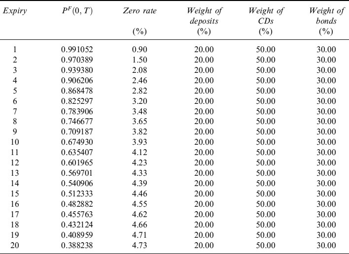
As a first step, we build the risk-free discount curve and the related term structure of zero rates. To generate such quantities we use a CIR model with values of the parameters and the starting instantaneous rate r0 as shown in Table 11.2.
The risk-free term structures of discount factors and zero rates are shown in Table 11.3, whereas a visual representation of zero rates13 is in Figure 11.2.
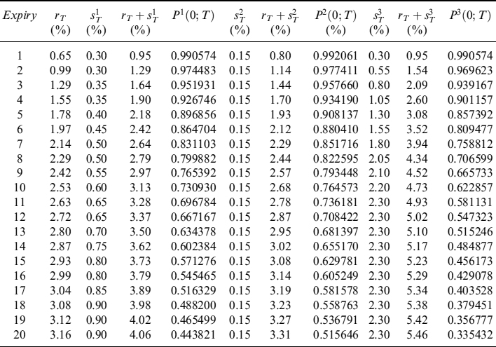
It is easy to build the term structures for the three sources by observing market prices and by forecasting reasonable expected spreads over the risk-free rate for each of them. Furthermore, we do not deal with the problem of how to bootstrap spreads from prices, but we simply take continuously compounded zero spreads over risk-free zero rates as given.
Let us start with the interbank deposit market: we build the related discount factor curve starting from zero rates for risk-free rate rT, adding zero-spread ![]() and then computing discount factor
and then computing discount factor ![]() . In Table 11.4 all the data for the three funding sources are shown: for example, for the interbank deposit market the zero-spread term structure is deterministic and time dependent, beginning at 0.30% for the one-year expiry and gradually increasing up to 0.90% for the 20-year expiry.
. In Table 11.4 all the data for the three funding sources are shown: for example, for the interbank deposit market the zero-spread term structure is deterministic and time dependent, beginning at 0.30% for the one-year expiry and gradually increasing up to 0.90% for the 20-year expiry.
Once the term structures of discount factors for each source have been built, it is straightforward to build the bank's funding discount curve as the weighted average of the different discount curves:
PF = {PF (0, t1),…, PF (0, tN)}
Table 11.3. Risk-free term structure of discount factors and zero rates
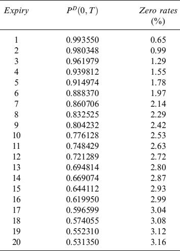
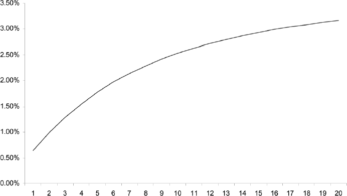
Figure 11.2. Risk-free term structure of zero rates
Table 11.4. Risk-free zero rates and interbank deposit (superscript 1), CD (superscript 2) and bond (superscript 3) market term structures of zero spreads, zero rates and discount factors
where each discount factor is defined as:
for i = 1,…, N.
Example 11.4.2. From the data shown in Example 11.4.1 it is possible to build the funding discount term structure, which is shown in Table 11.5 with the weight used for each funding source as well. In Figure 11.3 the zero rates of the three funding sources and of the bank's funding curve are depicted.
The funding curve can be used to discount the cash flows related to a loan (or to any other asset bought by the bank with a cash flow structure similar to a loan) so as to include in the pricing the average funding cost borne by the bank. In the case of deterministic spreads we have just examined, the average cost is the only cost to take into account, since it can be locked in at inception of the contract we want to price. In fact, the only risk is due to the stochasticity of market rates, which can be hedged by dealing in market instruments (such as FRAs and swaps); funding spreads, being deterministic, are not risk factors.
Clearly, the assumption of deterministic, though time-dependent, spreads is too naive and unacceptable in practice. Actually, spreads are just as stochastic as risk-free rates, and they are a function of the bank's (perceived) default risk and recovery ratios on the bank's bankruptcy, which depends on the type of instrument.
Table 11.5. Term structures of zero spreads, zero rates and discount factors for the bank's funding curve and weights for the three funding sources
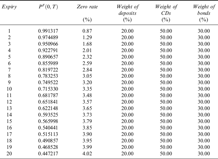
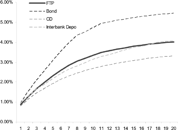
Figure 11.3. Term structures of zero rates for the bank's funding curve and the three funding sources
When spreads are stochastic, we can no longer assume that the funding curve is determined and fixed up to expiry tN, since the average life of the instruments underlying the different funding sources implies refunding risk, which can be defined as the greater-than-expected costs14 to be paid when rolling over a given funding source on future expiries. In fact, we cannot simply lock in the cost implicit in the risk-free curve and the spread curves by setting up a hedging strategy for all future refunding exposures, because we have contracts traded in the market enabling the treasury department to hedge risk-free rate risk, but it is almost impossible to hedge spread risk.
For example, the spread over the risk-free rate for bonds issued by the bank could be hedged by a credit default swap written on the bank's debt, but the buyer (and the seller) of such a swap cannot be the bank itself. Statistical hedging is possible by means of proxies that mimic spread evolution but we can no longer state that the cost of funding can be locked in completely today, so that the expected funding curve cannot be considered the only cost to include in the pricing of products sold to customers.
Remark 11.4.2. In the market it is possible not only to hedge exposures to the risk related to the risk-free (OIS/Eonia) rate, but also exposures to Libor (or Euribor for the euro) rates, since they are the underlying of FRAs and swap contracts. Libor/Euribor are not risk-free rates though, since they embed credit risk compensation for deposits used to lend to a primary bank in the interbank market. In fact, Libor/Euribor fixing quotes imply a spread over the risk-free rate which depends on the maturity of the corresponding deposit.
The bank's funding spread can be equal to or higher than that implied by Libor/Euribor fixings, so that what matters in reality is the volatility of the spread with respect to the Libor/Euribor rate, rather than with respect to the risk-free rate. In fact, the bank can hedge spread volatility partially (or even totally if its credit grade corresponds to that of a Libor/Euribor counterparty): the model we are presenting has to be modified accordingly and in case it is possible to fully hedge spread volatility, it boils down to the hypothesis of deterministic spreads seen before, since they can be locked in at inception of an investment.
We have to follow a different line of reasoning. First, we have to introduce a stochastic model for the different spreads, describing their evolution in time; second, we have to build spread curves for the chosen model, after fitting it to current market prices; third, we have to consider these curves as average funding costs for each funding source: then, we can also build an average bank's funding curve; fourth, we have to take into account that spreads may be different from the (implied) average or possibly higher than that on rollover dates, implying a higher cost to be borne by the bank.15 This higher cost can be considered an unexpected funding cost that has to be measured using a VaR-like approach and has to be covered by an amount of economic capital, in the same way as an amount of economic capital is provided to cover unexpected credit and market losses. Actually, this unexpected loss can be considered a market loss, although credit factors related to the bank contribute to it, in accordance with the analysis of Chapter 10.
In the case of bank default we choose a reduced-form approach, more specifically a doubly stochastic intensity model (see Chapter 8). Looking at this in greater detail, the survival probability of a bank between time 0 and time T is given by:
![]()
where default intensity λt is a stochastic process that is assumed to be defined by CIR dynamics:
We assume that correlation between instantaneous rate rt and default intensity λt is nil, although it is possible to design a model to include nonzero correlation. The probability of default is simply given by PD (0, T) = 1 − SP (0, T). In this setting, SP (0, T) has a closed-form solution given by (8.27).
In order to simplify calculation, for any funding source j we assume that after default a fraction Rj of the market value is immediately paid to the holder of the instrument issued by the bank: this is known as the recovery of market value (RMV) assumption and allows for a very convenient definition of instantaneous spread16 ![]() . The formula to compute the discount factor of spreads can easily be shown to be the same as for survival probability with a slight change in parameters, as indicated in formula (8.54), so that:
. The formula to compute the discount factor of spreads can easily be shown to be the same as for survival probability with a slight change in parameters, as indicated in formula (8.54), so that:
It is manifest that, in the setting in which we are working, what determines the actual spread of each specific source is the recovery ratio, the default intensity being the same for all of them. The recovery ratio in turn depends on the type of seniority of the funding source in the bank's balance sheet and on the ability of the bank's creditor to forecast it. We can suppose, for example, that the recovery ratio on CDs may be considered very high, either because of the seniority of the instrument, or as a result of the greater bargaining power of the bank with less sophisticated investors, or for their inabilit to attribute the correct level to it.17
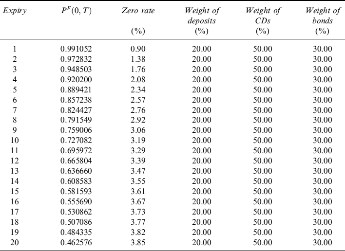
In the following example we recompute the term structures of the discount factors and zero rates for the three sources, by removing the assumption of deterministic spreads and by using the doubly stochastic intensity model with default intensity as in (11.17).
Example 11.4.3. In the doubly stochastic intensity model we use the values of parameters and initial level of intensity λ0 as shown in Table 11.6.
Table 11.6. Parameter and initial default intensity values used in the doubly stochastic default model to generate spread discount factors
| λ0 | 0.10% |
| Mean reversion speed Kλ | 0.75 |
| Equilibrium rate θλ | 2.00% |
| Volatility σλ | 17.00% |
We are now in a position to determine the zero spreads and total discount factors for each funding source. Zero spreads are derived from spread discount factors, computed with formula (8.27) considering the dynamics in (11.18). Total zero rate is simply the sum of the risk-free instantaneous rate plus the zero spread for the same maturity; the discount factor for the funding source is then calculated in a straightforward way.
For the interbank deposit market we assume that the recovery rate is R1 = 50%, for CDs R2 = 80% and, finally, for issued bonds R3 = 40%. The results are given in Table 11.7 for expiries running from 1 to 20 years.
The funding curve can be calculated by means of normal weighting and is shown in Table 11.8.
The difference between the funding curve generated by means of stochastic spreads and the one produced by deterministic spreads lies in that in the second case we have a curve of funding costs for each maturity which can be locked in at any future date, whereas in the first case we have a curve of funding costs that cannot be locked in by any hedging strategy, so that at any future date the curve implies only the expected cost to raise funds. It is clear that we have somehow to take into account both expected and unexpected costs, and hence post a suitable amount of economic capital to cover them. In the setting we have just specified this can relatively easily be done.
First we have to stress the fact that a part of the total funding cost using stochastic spreads can be locked in anyway. Actually, we can trade in hedging instruments written on the risk-free rate and that allows cancelling exposures to the risk-free component of future costs: this can be done for each source of funding. The stochastic part of the cost that cannot be hedged is only the spread and we have to compute its unexpected changes on scheduled refunding dates.
Table 11.7. Risk-free zero rates and interbank deposit (superscript 1), CDs (superscript 2) and bond (superscript 3) market term structures of zero spreads, zero rates and discount factors, assuming stochastic spreads. The recovery ratios for the three sources are, respectively, R1 = 50%, R2 = 80% and R3 = 40%

Table 11.8. Term structures of zero spreads, zero rates and discount factors for the bank's funding curve and weights of the three funding sources assuming a stochastic spread over the risk-free rate
To that end it is very useful that CIR dynamics have a known terminal distribution for instantaneous default intensity, namely a non-central χ2 distribution.18 This allows computing, at a given date, the maximum level (with a predefined confidence level) of default intensity λt and hence the maximum level of the spread and of the total cost for the refunding of each funding source. Additionally, we need the expected level of the spread to be the forward spread implied by the curve referring to each source; that is, for any t < t′ < T:
PSJ (0, T) = PSJ (0, t′)Et′ [PSJ (t′, T)]
which means that we want to compute the maximum level of the spread under a forward risk-adjusted measure.19 We then need a forward risk-adjusted distribution of default intensity (see equation (8.36)).
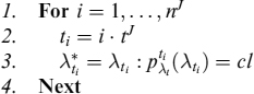
We now have all the tools to derive the unexpected funding cost associated with a given curve. Assume we still build an expected curve for each funding source up to expiry tN with an intensity model, as in Example 11.4.3. Further assume that each funding source J has duration tJ years, so that it entails a number of refunding dates tN/(tJ) − 1 = nJ. We follow the following procedure described in pseudo-code.
Procedure 11.4.1. We first derive the maximum expected level of default intensity ![]() , at scheduled refunding dates, with a confidence level c.l. (e.g., 99%):
, at scheduled refunding dates, with a confidence level c.l. (e.g., 99%):
Having determined the maximum default intensity level, we can compute the term structure of (minimum) discount factors for zero spreads corresponding to these levels:
Having the minimum discount factors for each expiry, we compute the total minimum discount factor for all expiries as:
for i = 1, …, N.
In building such curves we considered the cost of funding between two refunding dates is completely determined by maximum ![]() at the beginning of the period itself. In fact, we do not have any refunding risk and the curve is the same as if it had been derived using deterministic spreads.
at the beginning of the period itself. In fact, we do not have any refunding risk and the curve is the same as if it had been derived using deterministic spreads.
We take up Example 11.4.3 and show a practical implementation of Procedure 11.4.1.
Example 11.4.4. We start as before with the interbank deposit market and derive the maximum zero rates and minimum discount factors with a confidence level c:l. = 99%: they are shown in Table 11.9. In Figure 11.4 we compare the expected zero-rate term structure (from Table 11.7) with the maximum one: since the refunding schedule is yearly, the maximum term structure is smooth and similar in shape to the expected one.
We can do the same for the other two funding sources. In Tables 11.10 and 11.11 we show maximum zero rates and minimum discount factors for, respectively, the CD market and the bond issuance market; in Figures 11.5 and 11.6 we compare the expected zero-rate term structure (again, from Table 11.7) with the related maximum one. It is clear that the distance from the expected curve is much smaller for issued bonds, since they have a refunding schedule on a five-year basis, which allows fixing of funding costs for longer periods than the two-year basis for CDs and one-year basis for interbank deposits. The shape of the maximum zero rates for bonds is the most irregular, since it changes only every five years.
Table 11.9. Maximum default intensity and zero rates, and minimum zero-spread and zero-rate discount factors for the interbank deposit market at a confidence level of 99%
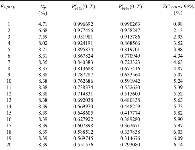
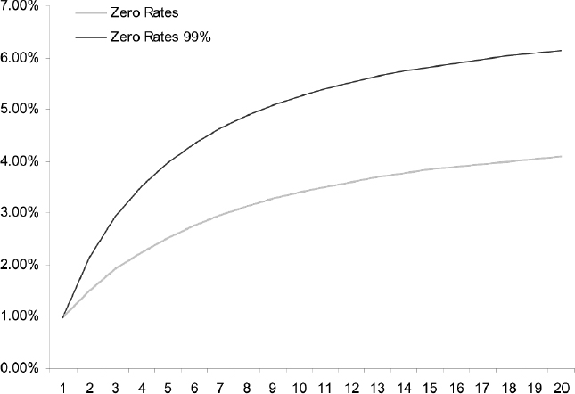
Figure 11.4. Term structures of expected and maximum zero rates for the interbank deposit market funding source
Table 11.10. Maximum default intensity and zero rates, and minimum zero-spread and zero-rate discount factors for the CD market at a confidence level of 99%
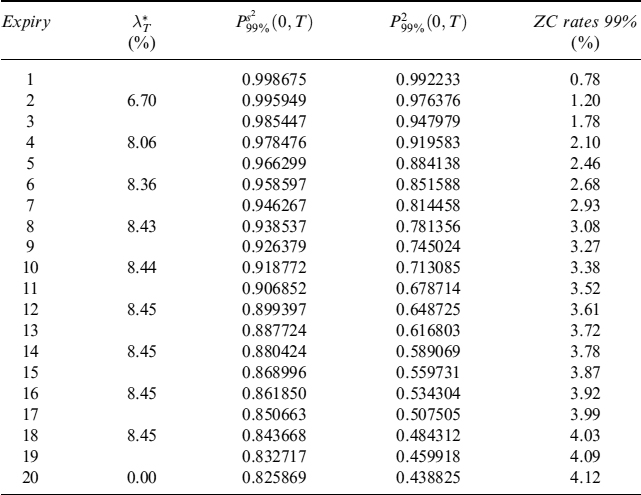
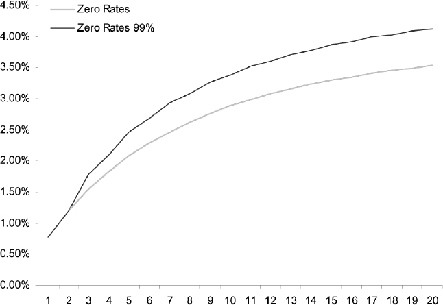
Figure 11.5. Term structures of expected and maximum zero rates for the interbank deposit market funding source
Table 11.11. Maximum default intensity and zero rates, and minimum zero-spread and zero-rate discount factors for the bond issuance market at a confidence level of 99%
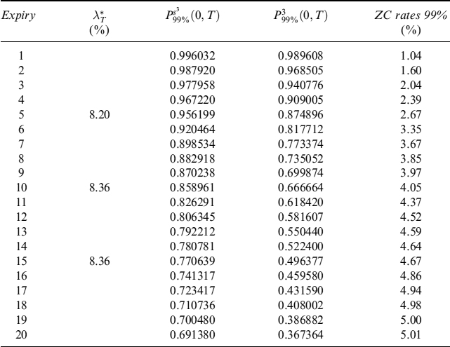
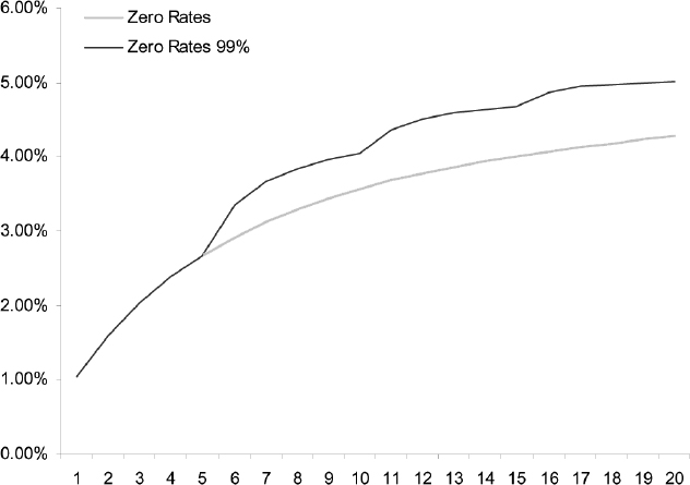
Figure 11.6. Term structures of expected and maximum zero rates for the interbank deposit market funding source
Table 11.12. Maximum zero rates and minimum discount factors for the bank's funding curve at a confidence level of 99%
The term structures of maximum zero rates and minimum discount factors for the funding curve can be computed as a weighted average of the corresponding term structures of the three funding sources. The results are shown in Table 11.12. Moreover, for the funding curve we compare the expected term structures (from Table 11.8) with the maximum zero rate term structure in Figure 11.7.
11.5 INCLUDING THE FUNDING COST IN LOAN PRICING
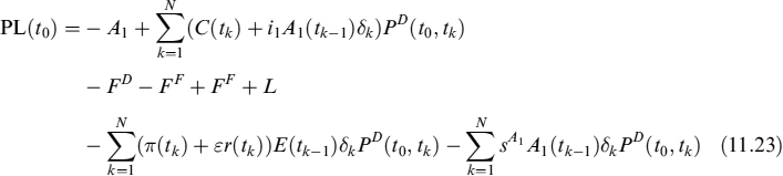
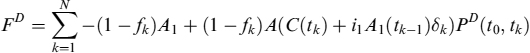
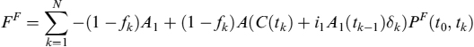
We sketched in Section 11.2 a very simplified balance sheet to stress the main factors affecting pricing of a loan. If we want to apply the expected and unexpected funding curve of Section 11.4 to the single-period setting in which we are working, formula (11.12) is still basically what we need to derive the fair interest rate to apply to the loan, but it is more convenient to express it in a slightly different way, so as to make easier its extension to a multi-period setting. In fact, after some manipulations we have:

where we have used the relationships shown in (11.2) and in (11.1); by further rearranging and by discounting where needed every addend by (1 + r) = 1/PD, so as to get the PL at time 0, we get:
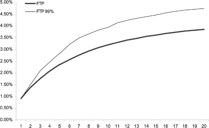
Figure 11.7. Term structures of expected and maximum zero-rates for the bank's funding curve

Equation (11.21) shows single-period profits and losses, discounted at time 0 by the risk-free curve. This way of expressing the PL allows easier calculation of fair interest rate ![]() for the loan, properly taking into account the funding costs and all the other costs related to credit, options, contingent liquidity and refunding. If we disregard the components relating to financial and liquidity/behavioural options and to contingent liquidity, in this setting the economic capital E is:
for the loan, properly taking into account the funding costs and all the other costs related to credit, options, contingent liquidity and refunding. If we disregard the components relating to financial and liquidity/behavioural options and to contingent liquidity, in this setting the economic capital E is:
![]()
This is equal to unexpected losses for credit events plus unexpected funding costs due to the difference between the expected and maximum funding curves (at the 99% c.l.).
It is worthy of note that since we are searching for fair rate ![]() making the PL equal to zero, the curve used for discounting is actually immaterial and can be chosen so as to make calculations as convenient as possible, although the theoretically correct curve belongs to the risk-free rate (see Chapter 10).
making the PL equal to zero, the curve used for discounting is actually immaterial and can be chosen so as to make calculations as convenient as possible, although the theoretically correct curve belongs to the risk-free rate (see Chapter 10).
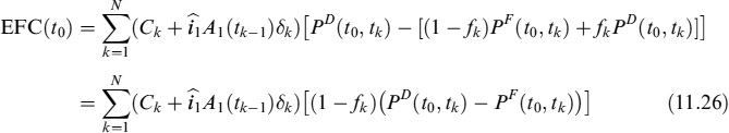
To generalize (11.21) to a multi-period setting, let us assume we are at t0 = 0 and asset A1, which is a loan, expires at tN and has a capital and interest payment schedule at dates t1,…, tN. We define the capital payment of loan A1 at time tk as C(tk) = A1(tk) − A1(tk−1), with A1(t0) = A1, A1(tN) = 0 and ![]() . Analogously, we define the liability payment schedule on the same dates as the loan and set D(tk) = L(tk) − L(tk−1), with L(t0) = L, L(tN) = 0 and
. Analogously, we define the liability payment schedule on the same dates as the loan and set D(tk) = L(tk) − L(tk−1), with L(t0) = L, L(tN) = 0 and ![]() . We can write a multi-period version of formula (11.21) as:
. We can write a multi-period version of formula (11.21) as:
The risk-free rate for each period is derived from the risk-free discount curve (PD (0, t) is the risk-free discount factor for date t):
![]()
where δk = tk − tk−1 is the accrual period. In the same way we can derive the risk-free rate from the risk premium curve π(tk), if this is time dependent. The fair (fixed) funding cost ![]() to pay on liabilities can be inferred from the funding curve:
to pay on liabilities can be inferred from the funding curve:

Let
and
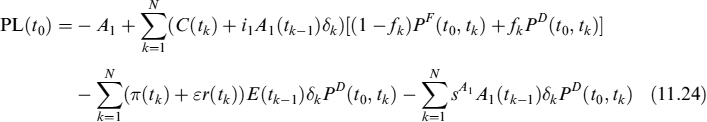
We rewrite equation (11.22) as follows:
Now, ![]() , which is the total liability needed to finance asset A1, net the fraction of equity used to cofinance the investment. Assuming perfect cash flow replicating funding, it is easy to check that
, which is the total liability needed to finance asset A1, net the fraction of equity used to cofinance the investment. Assuming perfect cash flow replicating funding, it is easy to check that
must both hold. So equation (11.23) can be rewritten as:
To determine fair rate ![]() we set PL(t0) = 0. The economic capital at each time tk is:
we set PL(t0) = 0. The economic capital at each time tk is:
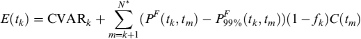
PF(tk, tm) = PF(0, tm)/PF(0, tk) is the forward discount factor derived from the expected term structure of the funding curve and ![]() is similarly defined. N* ≤ N is the number of periods that the financial institution deems reasonable to recapitalize the firm, should unexpected economic losses occur. The safest assumption is to set N* = N, so that the full economic capital needed up to expiry of the loan is taken into account. This is not what happens for other risks, though: for example, credit risk VaR is computed over one year and the posted economic capital can cover unexpected losses only for this period. Something similar could also be done for refunding risk.20
is similarly defined. N* ≤ N is the number of periods that the financial institution deems reasonable to recapitalize the firm, should unexpected economic losses occur. The safest assumption is to set N* = N, so that the full economic capital needed up to expiry of the loan is taken into account. This is not what happens for other risks, though: for example, credit risk VaR is computed over one year and the posted economic capital can cover unexpected losses only for this period. Something similar could also be done for refunding risk.20
Refunding risk VaR at time t0 is then:
which is the amount of unexpected costs generated by the contract's funding; by discounting economic capital, as in equation (11.24), we get the present value of these costs. On the other hand, the present value of expected funding costs can be derived from equation (11.24), by isolating the effects of funding. This is done in two steps:
- Derive fair rate
 of the contract without considering credit risk and economic capital, but still taking into account its participation in funding, by the following equation:21
- Value the contract with rate by discounting all cash flows with risk-free discount factors and subtract the quantity in equation (11.25). The value obtained in this way is the present value of expected funding costs:
which is a positive number.

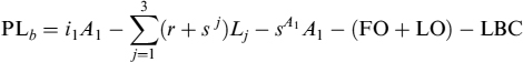
We will now present an example to demonstrate use of the tools developed in practice. To make things simpler we assume no credit risk, so that spread sA1 and the CVAR component in economic capital are nil: our example only includes unexpected costs related to refunding activity.
11.5.1 Pricing of a fixed rate bullet loan
Assume we want to price a bullet loan expiring at time tN with notional amount A1, paying fixed rate i1 at dates t1, …, tN. Capital is fully repaid at maturity, so that C(tk) = 0 for k = 0, …, N − 1 and C(tN) = A1. To compute the fair rate we apply formula (11.24) and we get:
where δj = tj − tj−1 is the accrual period and:
![]()
is the economic capital to cover refunding risk (we set N* = N). The fair rate ![]() is obtained be setting PL(0) = 0, so that:
is obtained be setting PL(0) = 0, so that:

where Pm(t, T) = [(1 − fT)PF(t, T)+fTPD(t, T)]. Given the relation between ε and f (see equation (11.1)), it seems that a circular argument is in formula (11.28). Actually, having defined percentage ε of the economic capital that the bank wishes to invest in the loan, we have that fk is linked to it via the following formula:
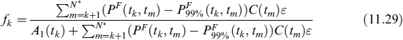
Example 11.5.1. We derive the fair fixed rate of a 20-year expiry loan, assuming we have the risk-free zero curve in Table 11.3 and the funding curves in Tables 11.8 and 11.12. The notional amount is A1 = 100 and it is paid back fully at expiry (bullet loan with no amortization schedule). We assume that the counterparty is not credit risky and we do not consider financial and liquidity/behavioural options and costs related to contingent liquidity.
We value the contract by assuming different percentages of economic capital's participation (ε) in funding. The results for the economic capital needed to cover refunding risk and the value for fk (i.e., the percentage of the asset that is funded by the capital at each period) are in Table 11.13. For example, ε = 0, economic capital is E(1) = 7.434 for the first year, gradually declining to 0.574 for the 20th year.
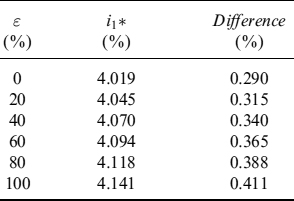
If there is zero capital investment in the loan (ε = fk = 0) then the fair rate is ![]() ; in this case it is also easy to compare the fair rate by including refunding risk, with the fair rate without refunding, which is
; in this case it is also easy to compare the fair rate by including refunding risk, with the fair rate without refunding, which is ![]() , so that the spread due to the economic capital for refunding risks accounts for
, so that the spread due to the economic capital for refunding risks accounts for ![]() . The fair spread for the other levels of ε are in Table 11.14.
. The fair spread for the other levels of ε are in Table 11.14.
Table 11.13. Economic capital and values of fk for a 20-year bullet loan for different levels of ε
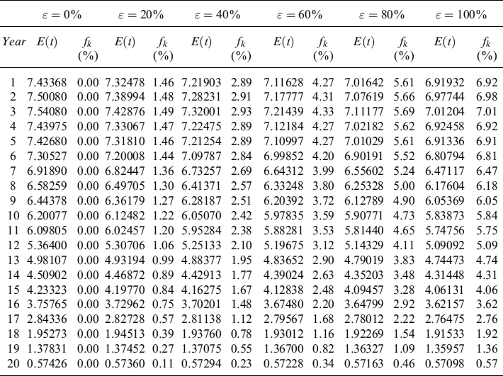
Table 11.14. Fair fixed interest rate for a 20-year bullet loan as a function of fraction ε of the economic capital invested in the loan and difference from the fair rate without refunding risk VaR ![]()
11.6 MONITORING FUNDING COSTS AND RISK CONTROL OF REFUNDING RISK
The framework outlined is suitable to monitor how expected funding costs evolve along with market movements of interest rates and funding spreads. Liabilities on balance sheets have their contract rates determined, so that the cost associated with them is known (at least as far as the spread over the risk-free rate is concerned), but rollover can occur under conditions for funding spreads different than expected. Economic capital, posted when deals are dealt, should be used to cover these unexpected costs.
Expected and unexpected funding costs change because the funding spreads paid by the bank change. In any event, the bank should also consider that the funding cost of liabilities on the balance sheet is locked in until the next corresponding rollover period. Monitoring economic capital is an activity the bank should operate on a regular basis, analogously with monitoring economic capital for market and credit risks using relevant VaR metrics. For funding costs, this risk-monitoring activity is focussed on the evolution of funding spreads in the market and computation of the amount of expected and unexpected funding costs, and checking at the same time whether the quantity of economic capital posted in the past is still enough to cover unexpected costs. Hence, economic capital for unexpected funding costs not only has to be included in the pricing of new contracts, but should also be monitored for existing deals.
Monitoring expected and unexpected funding costs mitigates the impact of distressed periods on:
- funding policies, because the bank does not have to change them as a result of an increase in costs that may be unsustainable without a suitable amount of capital to cover them;
- ongoing activity, because the bank does not have to suddenly stop its investment policies under stressed conditions for funding operations;
- profitability, since the bank can stabilize earnings using capital reserves to offset the volatility of funding spreads.
We now provide an example.
Example 11.6.1. We go back to the loan we priced in Example 11.5.1. Let us assume that the spreads paid by the bank over its funding sources suddenly rise. The CIR parameters fitting the new funding spreads are given in Table 11.15.
Table 11.15. Parameters of the CIR model used to calibrate new funding spreads
| λ0 | 1.10% |
| Mean reversion speed κλ | 0.75 |
| Equilibrium rate θλ | 3.00% |
| Volatility σλ | 17.00% |
The new funding curve will shift upward, but we still have to consider the fact that the funding has been locked for:
- 1 year on interbank deposits;
- 2 years on CDs;
- 5 years on bonds.
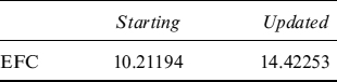
The original and the new zero-rate funding curve are shown in Table 11.16 and in Figure 11.8. In Table 11.17 we compare the first and the updated EFC after the increase in spreads. If economic capital does not participate in funding the deal (ε = 0), the EFC equal 10.21. This is the result of computing the present value of the loan, by discounting it by the risk-free curve, when it pays an annual coupon without refunding risk (i.e., 3.729%), which yields 110.212, and subtracting from this the value of the same loan obtained by discounting it by the funding curve, which yields 100.00. The expected costs increase to 14.42 from 10.21 with the new level of spreads: these are greater-than-expected costs which, should they occur, can be covered with the economic capital posted when closing the deal (7.43385).
Table 11.16. New expected and maximum funding curves after an increase in the funding spreads
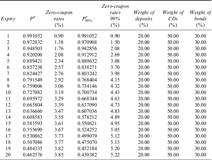
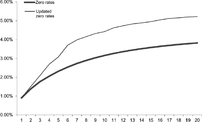
Figure 11.8. Term structures of funding zero rates with the starting and updated levels of the bank's funding spreads
Table 11.17. Expected funding costs before and after change in the bank's funding spreads
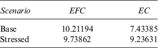
It is also possible to simulate distressed market or bank conditions entailing a different and more expensive composition of the funding mix. The liquidity buffer we analysed in Chapter 7 should be enough to prevent a change in the composition of the funding mix. Nonetheless, we have also examined suboptimal liquidity policies when funding gaps are more severe than implied by buffers. Within the framework just presented, the bank can measure any change in the funding curve to identify adverse changes in the funding mix. Example 11.6.2 deals with such a stress test exercise.
Example 11.6.2. Let us assume the bank starts with a funding mix producing the funding curves in Tables 11.8 and 11.12. The bank tests a stressed scenario resembling an idiosyncratic crisis: starting from the fourth year, its principal resort is interbank money market, with a weight changing from 20 to 40%; at the same time the weight for bonds experiences a sharp decline of 20%, from 30 to 10%. The resulting funding curve is shown in Table 11.18.
Table 11.18. Changes in the expected and maximum funding curves in a stress scenario similar to an idiosyncratic crisis
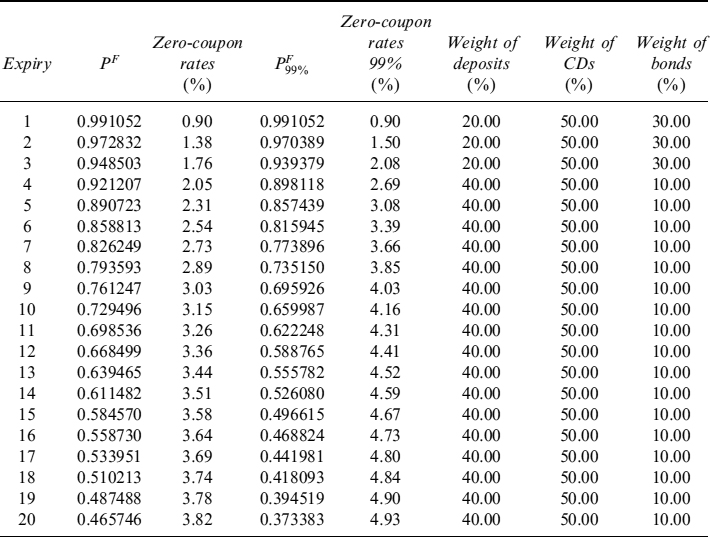
Table 11.19 shows the expected funding costs and economic capital at inception for the loan in Example 11.5.1 (notional = 100) and how they would be modified if the weights of each funding source alter after the fourth year under the distressed condition above. In the stressed scenario, on the one hand, expected funding costs decrease; on the other hand, economic capital to cover unexpected costs increases since the shorter maturities of interbank deposits imply more frequent rollover activity.
Table 11.19. Change in expected funding costs and required economic capital for unexpected funding costs in the stressed scenario of Table 11.18
11.7 FUNDING COSTS AND ASSET/LIABILITY MANAGEMENT
In Chapter 10 we introduced the main concepts underlying robust and consistent revaluation of the assets and liabilities on the bank's balance sheet. The main idea is to use a single, risk-free discount curve to compute the present value of future payoffs and of expected and unexpected losses and costs, thus allowing for clear decomposition of the total value of contracts and proper attribution to relevant departments. These ideas can also be applied to the framework we presented for funding costs.
Let us assume we have a marked-to-market balance sheet. At time 0, the bank closes a loan contract with a lender (e.g., an institutional investor) which is not charging any funding cost when setting the fair amount to lend. The amount is deposited in bank account D2, also risk free to avoid immaterial complications. Equity E is held in a risk-free deposit account D1. The balance sheet at time 0 looks as follows:
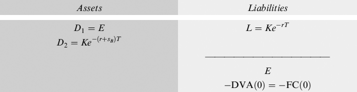
We now know (see Chapter 10) that DVA is not a reduction in the value of liabilities, rather it is the expected present value of funding costs the bank has to pay due to the fact that it is not a risk-free economic operator. As such, it has to be shown in the balance sheet as a reduction of the value of net equity, rather than of the risk-free present value of debt. The lending deal produces a P&L at inception of a loss equal to DVA(0) = FC(0) = e−rTK(1 − e−sBT), assuming that the LGD = 100%, so that instantaneous spread sB equals the instantaneous probability of default.
When buying asset A (e.g., lending money to a customer) the bank has to charge the FC it pays for the business activity to be profitable. Let us assume that the counterparty is default risk free, so that the bank does not have to charge any compensation for credit risk in the value of the asset. If the bank has enough bargaining power, the asset will be bought paying Ke−(r+SB)T. Revaluing this at the risk-free rate will produce a profit equal to FC, so that the balance sheet is:
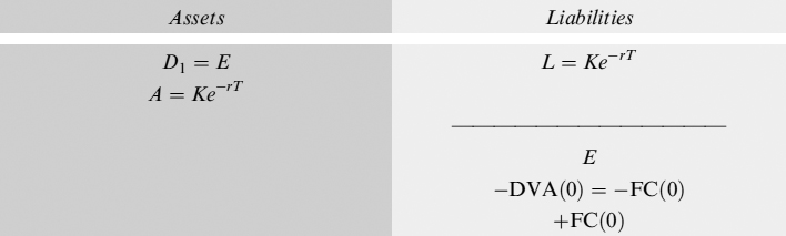
Funding costs can be split into an expected part EFC plus an unexpected part (computed at a given confidence level) covered by economic capital EC, which is absorbed from equity E. This part of equity needs to be remunerated at the risk-free rate plus a premium (r + π), so that the bank also needs to charge this cost when buying the asset (we assume no participation of economic capital to funding of the asset). When computing the present value of the asset by discounting everything at the risk-free rate, an extra profit will result equal to e−rTEC(0)e(r+π*)T − EC(0) (with π* chosen so that it will grant EC(0)e(r+π*)T − EC(0)erT = EC(0)e(r+π)T at time T), which will be used to compensate for remuneration of economic capital. The balance sheet at time 0 is then:
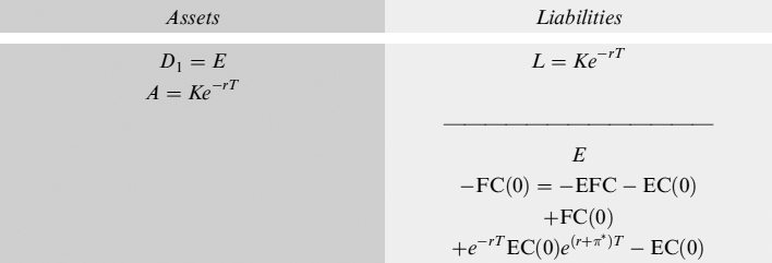
Economic capital EC(0) will be used only if unexpected costs actually occur, so that equity E will be abated for the corresponding amount. In any case, equity should be at least enough to cover them: E ≥ EC(0). The bank's stockholders are properly remunerated with profit EC(0)e(r+π)T at the end of the activity.
11.8 INTERNAL FUND TRANSFER PRICING SYSTEM
In theory, the framework sketched above should be used not only as a robust method to evaluate deals, but also should serve as the sound base for an internal system of FTP. We adopted an “industrial” approach in the design of FTP (see Section 11.2.1): in practice, having identified all the building blocks to evaluate a product, the business unit tasked with selling is charged the production costs by the relevant units involved in the production process.
When products are assets or off-balance-sheet commitments of the bank, it is quite obvious how to charge and assign single components of FTP. For example, for a typical banking book asset, such as a loan, total FTP is charged to the business unit tasked with selling, which will then pass these costs on to the counterparty (the bank's customer/debtor). Then FTP is split internally amongst the units involved in the production process as follows:
- the interest rate, the funding spread and the contingent liquidity components are paid to the treasury department;
- the credit spread is paid to the credit department;
- market and liquidity/behavioural options are paid to the ALM department;
- remuneration for economic capital is paid to the shareholders as dividends;
- the commercial margin is assigned to the business unit selling the loan;
- the non-financial margin is assigned to the operation/general services, IT departments.
While it is relatively clear how to determine and charge all the components in this case, when the bank tries to do the same with a product that is a liability, things are more complex and several solutions can be adopted. Products on the liability side of the balance sheet include funding sources (such as sight or saving accounts) whose counterparties are retail customers: when dealing with them the bank has strong bargaining power and typically is a pricemaker. More generally speaking, though, the problem of assigning components of the value extends to all kinds of liabilities (i.e., funding sources like long-term bonds not fully considered or not considered at all, products sold to customers since the bank has weak bargaining power and is often a pricetaker).
We should also stress that the problem with funding sources' FTP is of simpler complexity, since not all components enter the total price of the product. In fact, the credit spread cancels out the funding spread, so it does not have to be considered; moreover, the cost of contingent liquidity does not have to be considered since it is originated by the bank's investment in assets (in other words, by selling products that are assets), and not by liabilities.22 Commercial and nonfinancial margins can be charged (by paying a lower rate) only when the bank has enough bargaining strength.
Clearly, interest rate and funding components pose a problem that eventually boils down to whether the bank should use a single funding curve, or multiple funding curves to price all the contracts. We want to make it immediately clear that funding curves are effective rate curves that can only be used to quickly and easily incorporate funding costs in the value of typical banking book products, but they cannot be absolutely used to include funding costs in more complex (derivative) contracts23 and/or to include other components such as financial options or credit risk compensation. So, when we speak of multiple curves we are referring just to curves with different levels of funding costs embedded within and nothing else (i.e., no optionalities or contingent liquidity). These curves only serve the purpose of allocating profits and losses to business units – not to evaluate contracts, since we believe these should be evaluated by using the risk-free discounting curve in a fashion like that outlined in Chapter 10.
Moreover, given the general ideas put forward in Section 11.3, multiple curves are not related to assets, since the cost of funding assets is computed out of the weighted average of costs of different funding sources, condensed into a single curve that also takes the dynamic nature of the funding activity into account. It is true that in our framework there is a second funding curve, related to unexpected levels of funding spreads, but in reality this is always the same curve considered under different market conditions. So, when we talk of multiple curves we are always referring to different curves to evaluate the funding component of different liabilities.
There are many other variations on the multiple curve theme: we deem them inconsistent and highly misleading in terms of incentives and signals provided to business units, so we limit our analysis to two alternative solutions which we find acceptable and then flesh out their advantages and disadvantages.
11.8.1 Multiple curves
When multiple curves are used, the internal FTP system is based on:
- a curve used by the treasury department to include funding costs in the price of assets: this curve is representative of the weighted average of expected and unexpected costs over the different expiries;
- an evaluation curve for each type of contract in liabilities: these curves represent the fair rate the bank should pay for a given expiry on a specific funding source.
Let us go back to the framework presented earlier and to Example 11.4.1, where the curves used to evaluate liabilities are specific to each type of funding source (in the example there were three curves for interbank deposits, the CD market and bonds issued in the capital market). The weighted average curve to include funding costs in assets is that shown in Example 11.4.2.
When the bank designs the FTP system in such a way, the treasury department is remunerated for the total costs it pays to all funding units, which is a weighted average of the costs of single funding sources. Commercial units tasked with raising funds are remunerated for the cost they pay to the source providing funds. For example, a branch selling CDs to clients will transfer funds to the central treasury department, which will in turn pay interest to the branch (as shown in Figure 11.9 where the branch is the business unit raising funds from retail customers). Disregarding all possible margins that contribute to the profits of the branch, and focussing just on reconciliation of the unit's profits and losses, when the business unit transfers funds to the central treasury department ( arrows labelled C.F. in the figure), it will receive sufficient interest from the latter to fulfil contract obligations with its retail customers (arrows labelled l2). Hence the branch will eventually have P&L of zero (again, without considering any possible margin) and the cost related to funding is entirely borne by the treasury department. For other funding sources the mechanism is similar: the interest paid by the treasury department to single funding units is computed according to the curves related to each source (l1 and l3 in the figure).
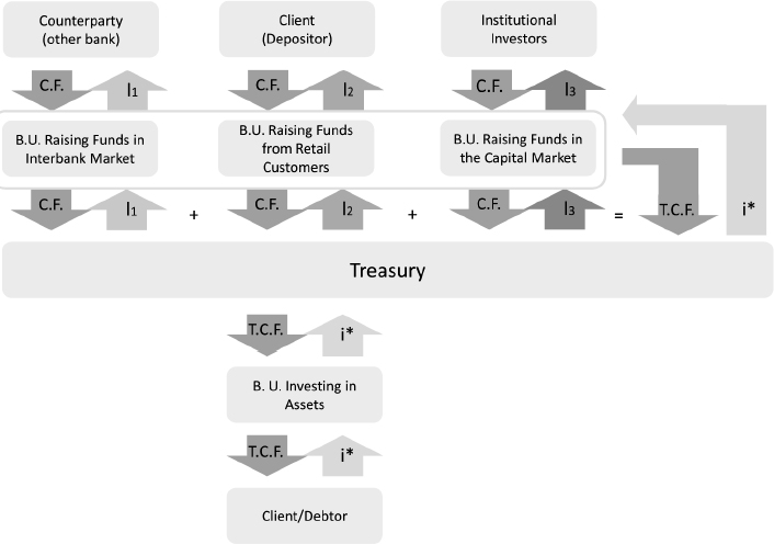
Figure 11.9. FTP system based on multiple curves
Total cash flow (T.C.F. in the figure) passed to the treasury department is the sum of funds raised by the funding units; the treasury department pays interest to single units such that total cost is i*.
In Chapter 10 we argued that the most correct and consistent way of evaluating all deals on the bank's balance sheet was to discount all expected cash flows, losses and costs using the risk-free rate curve. So, when revaluing liabilities using the risk-free curve, the treasury department will suffer a mark-to-market loss on each source, which was shown in Section 11.7 and in Chapter 10 to be the present value of funding costs.
The weighted average funding cost paid by the treasury department, originated by all funding sources, will then be charged to business units requiring funds for investments, such as loans. In Figure 11.9, the unit invests in its dealings with a client the money (T.C.F.) it receives from the treasury department. If the asset bought is a loan, the client will be a debtor to the bank and will pay an interest rate on the notional of the loan to the business unit, which will pass it on to the treasury department. Without considering commercial margins, credit risk and other components of FTP, the cost for liquidity is determined by the funding curve and will be included in the rate paid by the client. In Figure 11.9 it is indicated by arrows labelled i*.
By discounting assets using the risk-free curve, a positive mark-to-market P&L is produced (see Section 11.7), which has to be assigned to the treasury department so as to compensate it for weighted average funding costs. The P&L of the investing unit and of the treasury department will then be zero.
To recapitulate, an FTP system based on multiple curves, as far as the funding component is concerned, works according to the following rules:
- Each funding unit receives the interest it pays to the counterparty for the funds raised. Evaluating liabilities using the risk-free curve will produce a mark-to-market loss equal to expected funding costs EFC.
- The treasury department pays interest for the type of source used to raise funds to each funding unit. This will offset the loss in EFC for the unit, since it is passed to the treasury department.
- The treasury department will suffer a mark-to-market loss when evaluating all the liabilities equal to weighted average EFC.
- The investment business unit asks for funds from the treasury department and will be charged an interest rate compensating for weighted average EFC, i*, computed using the weighted average funding curve described above. The rate charged to the client will also include compensation for economic capital to cover unexpected funding costs that we have not shown in Figure 11.9.
- The investment unit will have a mark-to-market profit equal to the sum of EFC, which is passed to the treasury department, and remuneration for economic capital, which is passed to equity.
- The end result is that a P&L equal to zero is produced for the treasury department, the funding units and the investment unit.
The multiple curve approach has the following strengths: there is no distortion in investment and funding activity as a result of current market conditions since in the end no P&L is generated for any department involved. Funding sources will not be chosen by business units because of the spread they require. Incentives given to single units to increase the amount of funding from a specific source have to be given by means of external rules. These should be independent of current funding spread levels, so that the bank's management has more control in concentrating funding activity on certain sources (we will analyse this in greater detail in the next section). The weakness of the approach lies in the complexity of the mechanism and the amount of data to maintain.
11.8.2 Single curve
When a single curve is used, the internal FTP system relies on just one curve (i.e., the one used to include funding costs in the price of assets). As in the multiple-curve case, this curve is representative of weighted average expected and unexpected costs over the different expiries. Differently from the multiple-curve case, though, the same single curve is used to compute the fair rate to pay for all funding sources, without any reference to the actual rate paid by the funding units on the contracts they deal to raise funds.
The mechanism to allocate P&L amongst the bank's departments, when FTP based on a single curve is adopted, is shown in Figure 11.10. The main difference with respect to Figure 11.9 is in the interest paid by the treasury department to the funding units: a single rate i*, common to all sources, is received by the units, for the simple reason that a single curve is used in any event. The treasury department will bear a cost that is equal to the total funding cost for all funding sources, as in the multiple-curve case, but in this case single units will suffer a negative or positive P&L depending on the level of the actual spread they have to pay on the source used to raise funds.
For example, assume the single curve used is the FTP curve depicted in Figure 11.3. The business unit raising funds in the CD market has to pay an interest rate that is lower than the FTP curve, so it will receive interest i* and will pay interest l2 < i* to the client (depositor). By evaluating CDs using the risk-free curve, the mark-to-market loss representing expected funding costs implied in the curve of the CDs (the lowest curve in Figure 11.3) will be more than compensated by the interest received from the treasury department. The final result is that the business unit will have a positive P&L when raising funds from CDs sold to retail clients.
On the other hand, when the business unit raising funds in the capital market is considered, the amount of interest l3 paid to investors is higher than interest i* received from the treasury department. The mark-to-market loss of the bonds evaluated by the risk-free curve will not be compensated by interest paid by the treasury department, so the funding unit will end up with a negative P&L for conducting fundraising activity in the capital market.

Figure 11.10. FTP system based on a single curve
The treasury department will charge the total funding cost to the investing unit, as in the multiple-curve case. This will be total expected funding cost i*, as in the multiple-curve case, charged in the final rate passed to the client (which will also include compensation for the economic capital to cover unexpected funding costs, not shown in Figure 11.10). Hence the treasury department will be compensated for the total funding cost that it pays, on an aggregated basis, to the funding units and its final P&L will be zero. The same happens to the investment unit, which will pass the interest it receives from the client (debtor) to the treasury department and to equity.
To summarize, an FTP system based on a single curve that only analsyes the funding component and disregards all others, works according to the following rules:
- each funding unit receives an amount of interest computed on the basis of a single funding curve – not on the specific funding source curve. Evaluating each contract's liabilities with the risk-free curve will produce a mark-to-market loss equal to expected funding costs EFC, which will be more or less compensated by interest received from the treasury department depending on whether the funding source curve lies above or below the single funding curve used. So, fundraising activity generates a positive or negative P&L for the funding units depending on the type of source used;
- the treasury department pays the interest computed by the single curve to each funding unit. On an aggregated basis, the cost paid by the treasury department will always be the total funding cost for all sources, so it will suffer a mark-to-market loss when evaluating all the liabilities with the risk-free rate, equal to the weighted average EFC;
- the investment business unit asks for funds from the treasury department and it will be charged an interest rate that compensates weighted average EFC i* computed with the weighted average funding curve we described above. The rate charged to the client will also include compensation for the economic capital to cover the unexpected funding costs that we have not shown in Figure 11.9;
- the investment unit will have a mark-to-market profit equal to the sum of EFC that is passed to the treasury department and remuneration of economic capital passed to equity;
- the final result is that a P&L equal to zero is produced for the treasury department and the investment unit; a positive and negative P&L are produced for the funding units.
The advantage of the single-curve approach is that it is simple to implement and to maintain, especially when compared with the multiple-curve approach. On the other hand, it has the disadvantage of generating distortions in funding activity due to the P&L it produces for single funding units. These distortions may not always be welcome to the management of the bank.
For example, sight deposits are one of the cheapest sources of funding for the bank, since the interest rate paid by the funding unit is typically a fraction of the risk-free rate. Hence the funding spread is not just small, most of the time it is negative, thus contributing to abating the average and total cost of funding. Every time the business units raise funds from sight deposits in their dealings with retail customers, they receive an interest rate calculated on the single curve and make a profit. Similarly, units raising funds by selling bonds to institutional investors make a loss since the interest paid is above that implied by the single funding curve.
The single-curve mechanism creates, on the one hand, an incentive for the funding units to continue raising funds by dealing with retail customers through sight deposits; on the other hand, it discourages fundraising from institutional investors. Although this might be seen at first sight as a simple way to make the cost of single funding sources approach average cost and award a fair profit to the funding units that use less expensive sources, in reality it can generate a strongly imbalanced funding mix, with too high a percentage of short-term funding with retail customers.
In our opinion the multiple-curve approach is preferable since it does not create bias in funding activity by generating P&L. Specific funding policies can be implemented by adopting external rules, as we explain in the next section.
Example 11.8.1. In this simplified example we demonstrate how the multiple and single funding curve approaches work in practice. Let us assume that three funding units operating in the interbank, retail and capital markets raise funds for an amount of 100 each: all liabilities have a maturity of 1 year. The risk-free rate is 5% and the three sources have to be paid at a spread over it as shown below:
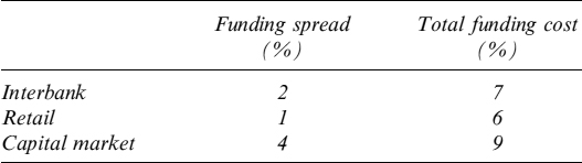
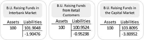
Figure 11.11. Balance sheet of the three funding units after having raised funds in the market
So, after 1 year the three funding units must pay back 107, 106 and 109, respectively. When these sums are evaluated with the risk-free curve (i.e., by discounting them at a risk-free rate of 5%), the mark-to-market value is inserted in the liabilities of each unit as shown in Figure 11.11. If business units were separate and independent firms, they could invest sums raised at the risk-free rate in a riskless investment earning 5%, so that the present value is 100, and this is what appears on the asset side of the balance sheet of single units. In this case each unit would suffer a loss inserted in the marked-to-market balance sheet as shown in Figure 11.11.
In reality, the three funding units transfer funds to the treasury department. Let us assume that the FTP hinges on a multiple-curve system: each funding unit will receive the interest it has to pay to its creditor, so it invests in the treasury department the funds raised at the same rate it pays on liabilities. Hence, the value of assets on the balance sheet of each funding unit now equals the value of liabilities (as shown in Figure 11.12); this will clearly produce a zero P&L for all the funding units.
The treasury department collects funds from the three units and shows a liability on its balance sheet equal to the present value of the funds raised by them (i.e., 101.9047 + 100.9523 + 103.8095 = 306.6667). Were the treasury department an independent firm, it could invest total raised funds in the risk-free rate, so that the present value of its asset would be 300 (as shown in Figure 11.12). In this case the treasury department would record a loss on its marked-to-market balance sheet.
But the treasury department transfers the funds to the investment unit and charges the total funding cost it has to pay to the single funding units (i.e., (7% + 6% + 9%) × 100 or 7.33% × 300). The investment unit, in turn, will charge this cost to the counterparty, so that the present value of its assets and liabilities match, both being equal to 306.6667, thus producing zero P&L. Furthermore, the present value of the assets on the treasury department's balance sheet now equals 306.6667, so that its P&L is also zero. All this is shown in Figure 11.13, along with the aggregated balance sheet of the bank: clearly, since the bank as a whole raises 300 which it invests in an asset charging total funding costs, the present value of assets and liabilities are the same and total P&L is zero.
Let us now assume the bank structures the FTP system such that it is based on a single funding curve. The three funding units raise funds on the market and transfer them to the treasury department. Each funding unit then receives remuneration common to all funding sources, which we suppose equal to the average funding cost (i.e., (7% + 6% + 9%)/3 = 7.33%). The balance sheets of the single units are shown in Figure 11.14: comparing them with the balance sheets in Figure 11.13, it can clearly be seen that the FTP mechanism now generates a P&L for each funding unit. The units working in the interbank and retail markets, paying their creditors less than the average funding rate credited to them when transferring funds to the treasury department, will mark a profit in the marked-to-market balance sheet. The funding unit working in the capital market will suffer a loss, since the funding costs it pays are higher than the average rate credited.
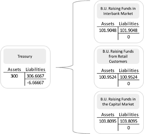
Figure 11.12. Balance sheet of the three funding units and of the treasury department after internal transfer of raised funds (FTP is based on multiple funding curves in this case).
The treasury department is unaffected by the single funding curve mechanism: its total cost is still the same, 7.333% × 300, so that the present value of all its liabilities is the same as when the bank adopts a multiple-curve based FTP. Moreover, the transfer of funds from the treasury department to the investment unit is unaffected by the single-curve choice, so that the balance sheet and the P&L are the same as in the multiple-curve case. At an aggregated level, the bank balance sheet is also unaffected.
This example confirms what we affirm in the main text: the choice between a single or multiple-curve FTP is important only for P&L attribution of the funding units, otherwise it is quite immaterial.
11.8.3 Implementation of funding policies
The framework described above takes as given the number of funding sources and their weight in the funding mix. We now also know how to assign the funding costs amongst funding and investment units, via the treasury department, and how finally to charge them to the client (debtor). We now examine how to implement a funding policy, with given targets in terms of composition of the funding mix and possibly of total cost paid for funding.
It is very likely that the bank has more bargaining power on some funding sources (e.g., those sold to retail customers) than others (e.g., bonds issued). This usually means the most effective way to abate the total funding cost is to act on the funding mix, by identifying less expensive costs and by incentivizing business units to sell those funding products whose weight in the mix is lower than targeted and not to sell those products whose weight is higher. As suggested before, the best way to do this is by using a set of rules separated from the FTP system. One possible solution, provided the bank adopts a multiple-curve approach,24 is the following.
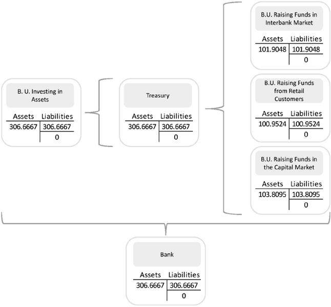
Figure 11.13. Balance sheets of the three funding units, the treasury department and the investment unit after internal transfer of raised funds (FTP is based on multiple funding curves in this case)
Assume the target average funding cost is given by the funding curve:
where ![]() is the targeted weight for funding source j. If the business unit, when raising funds and transferring them to the treasury department, is given back not only the interest it has to pay, but also an extra payment:
is the targeted weight for funding source j. If the business unit, when raising funds and transferring them to the treasury department, is given back not only the interest it has to pay, but also an extra payment:
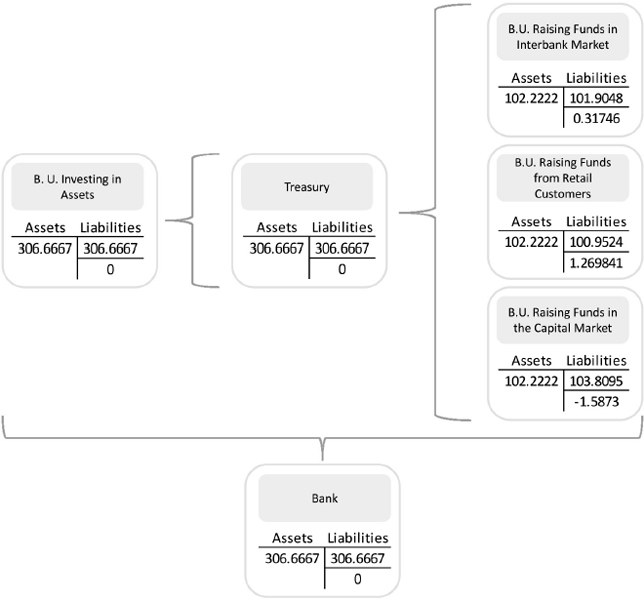
Figure 11.14. Balance sheets of the three funding units, the treasury department and the investment unit after internal transfer of raised funds (FTP based on single funding curves in this case)
then the funding units make a positive P&L which is proportional to the distance of the actual weight from its targeted value. Looking at this in greater detail:
- if the source is underweighted
 , then the total payment transferred from the treasury department will be higher than the interest the unit has to pay and it will earn a profit;
 - when the source is overweighted
 , there should be no incentive so that no extra amount is paid to the unit.
This is a very simple rule and much more complex rules can be designed to help the bank reach its target.
The problem we now have is whether incentives have to be charged to the treasury department or to some other department. In theory, if the funding policy is not strictly decided by the treasury department, as usually happens in banks, but by top management, these costs are ultimately borne by the shareholder. In practice, the bank may decide to assign these implementation costs to the treasury department, which in turn will charge them to the investment units. These will finally charge costs in the pricing of products sold to customers.
We believe rules designed as above are more effective than the incentives and disincentives implied in a single-curve based FTP. It should be noted that the rule presented above creates an incentive based on the target weight – not the cheapness/expensiveness of the funding source with respect to the average funding source: we already briefly alluded above to the unintended consequences that this second type of mechanism can produce.
11.9 BEST PRACTICES AND REGULATION
We argued at the beginning of this chapter that prevailing best practices, as far as funding costs are concerned, should be considered antiquated and inadequate for the current financial environment.
The basic principle to account for funding in a new investment is so-called marginal cost or matched maturity: it is the cost paid by the bank to raise funds in the market (usually the capital market) with the same maturity as the investment. This rule, although considered by many practitioners and some surveillance authorities as sound practice, has many drawbacks.
First, this is far removed from the actual funding activity of the bank, which uses a mix of funding sources – not just bond issuance in the capital market. Second, for investments expiring after 10 years, the bank is unable to raise funds with a matched maturity, not even by issuing bonds. This means that the marginal cost in this case would be an assumption based on extrapolation of the funding costs paid by the bank on existing liabilities.
The framework presented above recognizes that the matched maturity rule is in theory the correct way to include funding costs when valuing an investment; at the same time it also improves the rule and eliminates the two drawbacks we mentioned. In fact, it considers a mix of sources that contribute aggregately to the funding of investments; additionally, it takes liability rollover activity into account, which in many cases cannot be avoided by the bank. This activity implies a refunding risk (i.e., a greater-than-expected funding cost) that is explicitly measured and included in the pricing, without pretending that the bank can always fund its assets with liabilities of equal duration. Actually, our framework hinges on the marginal cost, matched maturity principle, although it extends it to all components of the funding mix (and does not limit it to bonds) and to the dynamic nature of fundraising activity.
On the assumption current practices need to be revised, the ideas presented in this chapter and, more generally, in the entire book need to be verified as compliant with current regulation. We start with Basel regulation and the document Principles for Sound Liquidity Risk Management and Supervision [99]. The document does not deal in depth with FTP, but there is mention of it in Principle 4:
“A bank should incorporate liquidity costs, benefits and risks in the internal pricing, performance measurement and new product approval process for all significant business activities (both on- and off-balance sheet), thereby aligning the risk-taking incentives of individual business lines with the liquidity risk exposures their activities create for the bank as a whole.”
This principle seems to confirm the general setting we have outlined above, including liquidity buffer costs too, although it is so generic that alternative approaches can also be suggested. In the comments to Principle 5, the document reads:
“A bank should consider the interactions between exposures to funding liquidity risk and market liquidity risk. A bank that obtains liquidity from capital markets should recognise that these sources may be more volatile than traditional retail deposits. For example, under conditions of stress, investors in money market instruments may demand higher compensation for risk, require roll over at considerably shorter maturities, or refuse to extend financing at all.”
The interconnection between liquidity and market risks is captured in our framework by the volatility of funding spreads. The volatility of capital market sources more likely refers to the amount to roll over (and hence to funding gap risk) rather than to funding spreads, but in reality the consideration can be applied to both.
FTP is given much fuller treatment in the EBA's documentation Guidelines on Liquidity Cost Benefit Allocation [7], the key goals of which are:
- development of an adequate and comprehensive pricing mechanism;
- the mechanism should incorporate all relevant liquidity costs, benefits and risks; and
- the resulting mechanism should allow management to give appropriate incentives to ensure prudent management of liquidity risk.
Furthermore, [7] goes on to point out:
“The funding transfer price concept in this paper consists of two components. First, at a minimum, the costs of raising funds from an asset and liability management perspective and the interest rate curve cost component (direct costs of funding) should both be captured. Second, to calculate the correct fund transfer price, indirect liquidity costs are to be added.
Amongst these liquidity costs, one should at least distinguish between (i) the mismatch liquidity cost, for which, the liquidity tenor (not the interest rate tenor) is relevant*; (ii) the cost of contingent liquidity risk, including inter alia, the cost of holding stand-by liquidity available to cover unexpected liquidity needs (liquidity buffer) as well as the cost of roll-over risk; and (iii) other categories of liquidity risk exposure that an institution may have e.g. a country risk cost that may arise for institutions where balance sheets in non-fungible currencies are being funded.”
Indirect liquidity costs include not only those related to the liquidity buffer, but also rollover risk, which is meant to be the risk related to unexpected funding costs if the phrase is but an alternative way to refer to the liquidity buffer. Additionally, the footnote is fully in line with the our proposed approach.
The EBA's Guideline 5, “The internal prices should be determined by robust methodologies, taking into account the various factors involved in liquidity risk” supports decomposition of FTP suggested in this chapter. Moreover, in the comments by the EBA following the statement, the components of the transfer prices they present strongly resemble those listed in Section 11.2.
As far as incentives are concerned, the EBA's document seems to indirectly agree with our view, since “if management wishes to incentivise certain behaviours, this should be subject to a separate, formal approval and reporting process.”. We interpret this as FTP should not implicitly or explicitly incorporate incentives on a systematic basis.
Finally, the need for complex quantitative modelling is indicated in the comments to Guideline 5:
“Selecting an internal pricing yield curve is a critical aspect since it determines how profit contributions to net interest rate margin are measured. … For maturities exceeding that of an institution's securities having the longest maturity, the curve may be calculated using an interest rate term structure model. When appropriate and with respect to the proportionality principle, institutions should use internal funding cost curves broken down by currencies.”
In the first draft of the document (known as EBA CP36), the last comment on Guideline 5 reads as follows:
“The internal prices used should reflect the marginal cost of funding. The price should reflect the marginal cost over a homogenous product group as an average, but it should also reflect current costs. Funding already acquired (tapped) should already be taken into account in the prices of products sold (or being sold). To achieve a reliable marginal funding cost, an institution should be able to adjust transfer prices according to current demand for new funding, mainly, when calculating the contingent liquidity cost price. As the required size of the liquidity buffer (and its cost) changes with any new product sold, as well as any new funding tapped, an institution should ideally be able to recalculate the transfer price according to its expected balance sheet term structure (Dynamic Price Setting).”
This was basically a short description of the framework we presented. The final version of the document, although not modifying opinion, is shorter and open to a different view, since it now reads:
“The internal prices used should reflect the marginal cost of funding26. The prices should reflect the marginal cost over a homogenous product group. As the required size of the liquidity buffer (and its cost) changes with any new product sold, as well as any new funding tapped, an institution should ideally be able to recalculate the contingent liquidity cost element of the transfer price.”
In conclusion, the approach we proposed above is not in contrast with any suggestion, recommendation or guideline provided by international regulators.
Amongst national regulations, in a letter sent to all institution treasurers the British FSA [11] highlighted the importance of consistent fund transfer pricing practices. In the letter, the FSA takes a clear stance against the weighted average approach:
“Of the firms surveyed, 5 charged FTP by reference to the weighted average cost of funding either already on balance sheet or projected in an annual budget process. This cost was expressed as a reference rate plus spread, which was then applied to business line balance sheets, irrespective of duration. This methodology in isolation lacks sufficient flexibility for the FTP framework to be used to incentivise or discourage business behaviour and appropriately charge for the duration of risk. This was demonstrated in some cases in 2007 with the buildup of large inventory positions in certain asset classes, where returns were not commensurate with risk taken, and in the onset of volatile conditions where marginal costs rose sharply and the FTP regime did not appropriately reflect market conditions to business lines.”
The point to stress is that the approach “in isolation” lacks of flexibility to direct business behaviuor, but this does not mean it cannot be improved and embedded in a richer and more complex framework to properly account for all relevant risks. Moreover, we believe the same lack of flexibility is also suffered by a pure marginal cost approach, taken in isolation. We do not believe that the poor performance of the FTP systems alluded to by the FSA is due to some banks adopting a weighted average approach, but rather that it is the result of the more structural flaws of designed systems.
1 We adopt a uniform terminology both for derivative and standard banking contracts, so we apply the term CVA to a loan as well, although it is primarily used to adjust the value of a derivative contract to account for expected credit losses.
2 See [93] for a discussion on passive and productive risks. Very briefly, productive risks are those that cannot be hedged or diversified away by the bank, whereas passive risks can. Only productive risks related to banking activity should absorb economic capital and then generate a corresponding remuneration; passive risks, on the contrary, should be properly hedged or diversified away and no capital should be allocated to cover them, since they are not strictly inherent to the banking business: an investment does not have to produce a remuneration of economic capital for these types of risks.
3 This is not totally true since credit derivatives are available in the market, with underlying issuers being major companies in most economic sectors. Clearly, when it is possible to hedge credit risk with such instruments, unexpected losses should not be considered since the risk can be thought of as passive – not productive. For most retail business (i.e., mortgages, loans to small corporates, etc.) the risk is generally productive.
4 Recall that B is a risk-free asset, so no loss can result from default, liabilities cannot be evaluated by including the default of the bank (see Chapter 10 for a discussion) and from the bank's point of view they are default risk-free securities.
6 See Chapter 9 for behavioural models and related risks.
7 Most bank bonds expire within 7 years, although longer maturities are not impossible to find in the market.
8 We are conscious of stating something that many operators, including some surveillance authorities, will consider opposite to best practices. Nevertheless, we strongly believe best practices inherited from the past need deep and serious revision, because either they are based on premises no longer valid in current markets or they are based on hypothetical funding activity the banks could neither operate in the past nor can they today. Although best practices from the past seemed apparently safe and sound, they hid many assumptions that must now be made explicit, analysed and taken into account in risk measurement and management.
9 See Section 8.3.3.
10 In Chapter 10 we studied the relationship between the spread seen as credit risk compensation on one side and funding cost on the other.
11 We may refer to the funding cost related to a given source as total interest plus possible implicit costs or optionalities. It is frequent, though, to consider funding cost just as the spread over the risk-free rate.
12 We recall that the risk here refers only to unexpected cost of rollover (refunding risk) – not the amount to be renewed (gap risk).
13 Worthy of a quick mention is the fact that zero-rate rT associated with discount factor PD(0, T) for given maturity T is calculated as rT = −ln(PD(0, T))/T.
14 Expected costs are those implied by the discount (or, equivalently, zero rate) curve of the funding source.
15 Basically, we may experience future spreads higher than the forward spreads implied in the curve.
16 See Section 8.4 and [63].
17 This is a convenient point to mention that for some funding sources, such as demand or saving deposits, the spread is much more under the bank's control and often can be modelled just as a function of short-term market (either risk-free or treasury) rates (see Chapter 7 for the fair rate to apply to non-maturing liabilities). Since this case is similar to that of deterministic spreads presented above, we do not include such sources in our setting, although they do contribute in practice to average down the total funding cost of the bank.
18 A non-central χ2, with d degrees of freedom and non-centrality parameter c, is defined as the function χ2(x; d, c). See Chapter 8 for more details.
19 Superscript t′ to the expectation operator E[·] means that we are working in a t′-forward risk-adjusted measure. Technically speaking, we are calculating expectations by using bond PsJ (0, t′) as a numeraire.
20 If the bank calculates economic capital for a horizon shorter than the duration of the contract, the pricing could not be sufficient to remunerate the greater amount of capital needed if unexpected losses exceed those related to the chosen period. This is why we suggest including the full amount of economic capital in the pricing, even if it is not allocated entirely at inception of the contract.
21 See equation (10.1) for a simplified version of the formula we are presenting here and for a discussion on funding costs.
22 The only case in which a buffer is not originated by assets is that of nonmaturing liabilities, but this is due to the bank offering an interest rate on them, based on a behavioural rather than a financial criterion (sight deposits should be remunerated using a zero interest rate). See Chapter 7 for more details.
23 See Chapters 10 and 12.
24 The analysis of this section can also be applied to the single-curve approach, but in a more complicated way.
* “For example, if a 3 year fixed rate loan is granted and is funded by 3 month commercial paper that will be rolled over each quarter, the appropriate liquidity cost is the 3 year funding cost and not the initial 3 month cost of CP issued.”
* “Cost of making new funding transactions in the market.”