
1 Introducing Logic Pro X
FOR YEARS, LOGIC HAD A REPUTATION FOR BEING VERY COMPLEX. Over the last few versions of Logic, however, that situation has improved dramatically. With each new version, incredible new features have ensured that Logic maintained its place as an industry leader. Logic Pro X is no different in that regard. It is an incredibly deep, powerful, and feature-rich recording and production application that you can have up and running quickly. It has a unique and highly customizable set of tools that allows you to configure a workflow that suits your “logic.” Its editing and processing tools are second to none, and its suite of effects and software instruments is truly complete. In this chapter, you’ll learn what Logic is, where it’s from, and its basic working premises.
What Is Logic Pro?
If you hear people discussing Logic, you’re likely to hear terms such as “professional,” “powerful,” “flexible,” and “steep learning curve” thrown around. So what is Logic Pro, really?
Put simply, Logic Pro is the most flexible, powerful, comprehensive, professional, and elegant application for producing music on a computer. Although some may consider that a rather contentious statement, after reading this book you will probably at least concede that this claim is not outrageous. A number of other powerful, professional, and worthy music-production programs are on the market today. I don’t mean to downplay their functionality. Some applications have a feature or two that Logic lacks, or they implement one of the features that Logic also includes in a way that some prefer. Logic does, however, offer the best combination of features, flexibility, and power of all available music production applications.
Logic offers you:
![]() Audio recording: Record audio directly into Logic.
Audio recording: Record audio directly into Logic.
![]() Audio editing: Edit audio files using Logic’s many editing tools, including sample-accurate editing, Flex Time, and Flex Pitch in the Tracks area.
Audio editing: Edit audio files using Logic’s many editing tools, including sample-accurate editing, Flex Time, and Flex Pitch in the Tracks area.
![]() MIDI recording: Record and play back MIDI information.
MIDI recording: Record and play back MIDI information.
![]() MIDI editing: Edit MIDI information in one of several MIDI editors.
MIDI editing: Edit MIDI information in one of several MIDI editors.
![]() MIDI notation editing: Edit and print out professional scores and music charts.
MIDI notation editing: Edit and print out professional scores and music charts.
![]() Browsers: Manage all your multimedia files right in the Logic Pro main window.
Browsers: Manage all your multimedia files right in the Logic Pro main window.
![]() Global tracks: Easily set up and edit project arrangement, marker, tempo, key signature, transposition, beat mapping, and video frame information.
Global tracks: Easily set up and edit project arrangement, marker, tempo, key signature, transposition, beat mapping, and video frame information.
![]() Software instruments: Use software instruments from within Logic.
Software instruments: Use software instruments from within Logic.
![]() Library: Access complete channel strip settings and patches for your tracks in the Logic Pro main window.
Library: Access complete channel strip settings and patches for your tracks in the Logic Pro main window.
![]() Arranging: View all your song elements as graphic regions and arrange them visually.
Arranging: View all your song elements as graphic regions and arrange them visually.
![]() Mixing: Mix your audio tracks and your MIDI tracks within the same song using Logic’s completely customizable Mixer.
Mixing: Mix your audio tracks and your MIDI tracks within the same song using Logic’s completely customizable Mixer.
![]() Processing: Use Logic’s professional offline and realtime processors and functions.
Processing: Use Logic’s professional offline and realtime processors and functions.
![]() Control surface support: Configure any hardware MIDI controller to be a hardware controller of any Logic function.
Control surface support: Configure any hardware MIDI controller to be a hardware controller of any Logic function.
![]() Environment: Build an entire virtual studio and processing environment inside Logic.
Environment: Build an entire virtual studio and processing environment inside Logic.
For these features and more, Logic has earned its well-deserved reputation as the most complete professional music production application, and it continues to break new ground. What about that talk of Logic’s steep learning curve? As with most applications that are as deep as this one, it helps to know the application’s internal workings to more readily understand how to use it. To give you a solid grounding in the fundamental concepts of Logic, I’ll start at the very beginning with Logic’s origins and see how the functionality of those previous applications relates to the current version of Logic.
A Brief History of Logic
Once upon a time, in the mid-1980s, during what now would be considered the “prehistoric” era of computer music, a small German software company named C-LAB created a Commodore 64 program called Supertrack. Supertrack, like all early sequencers, was designed to allow users to store, edit, and play back the notes and performance information generated on MIDI synthesizers. (See the section “A Brief Overview of MIDI” later in this chapter for an explanation of MIDI.)
By 1987, this basic program evolved into Creator, and finally into Notator. Notator, which ran on the Atari ST, added a musical notation (or musical score) editor to Creator and became an instant power player in the burgeoning field of computer-based MIDI sequencers. Notator offered a clean, simple interface for four powerful MIDI editors: a realtime musical notation editor, an Event editor for displaying MIDI information in a scrolling list, a Matrix editor for displaying notes graphically, and a Hyper editor for editing non-note MIDI data (such as pitch bend). With these editors, you could play a song on your synthesizer or program it on your computer from scratch, then rearrange, edit, and manipulate your data as sheet music in the notation editor, in a text list, a graphic “piano roll,” or a bar graph–style display.
As you can see in Figure 1.1, which shows an edit screen from the final version of Notator for the Atari, the program used the very same concepts and offered many of the same tools for manipulating MIDI information that are still used today. Notator’s extensive editing options gave musicians powerful tools for creating and arranging music in an easy-to-use package. Notator won rave reviews from power users and hobbyists alike, and garnered a huge following among early MIDI musicians. Even 20 years after its final version, Notator still has a very lively following. In fact, there are websites and mailing lists on the Internet for people who still use Notator today.
Figure 1.1 This screenshot from Notator Version 3.2.1 shows the Matrix and Event editors. Users of Notator would feel right at home with the evolved Matrix and Event editors of Logic, which are fundamentally the same two decades later.
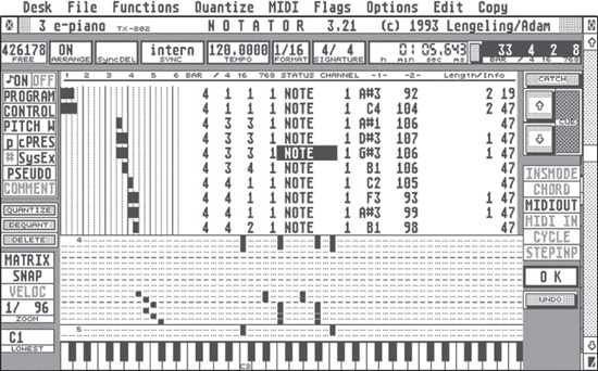
© The Notator Users Group (www.notator.org).
By 1993, the principals who developed Notator left to form their own company, Emagic, and built upon their previous efforts by adding a graphical arrangement page and object-oriented editing, among other innovations. This product was named Notator Logic, and later simply Logic. Logic was soon ported to run on the Macintosh computer, which was quickly overtaking the Atari as the music computer of choice for professionals. This early version of Logic introduced the basic architecture and concepts that would form the basis for future iterations of Logic.
By the late 1990s, Logic’s developers had ported Logic to run on Windows computers as well as the Macintosh, quietly discontinued the Atari version, and added to the program the ability to record and edit audio in addition to MIDI. To signify this, the developers modified the name of the application to Logic Audio. By the end of the 1990s, there were three versions of the application, each with an expanded feature set. Logic Audio Platinum had the most professional recording options, offering the most hardware options, including unsurpassed support for Digidesign’s industry-standard hardware, Pro Tools TDM. Logic Audio Platinum became nearly ubiquitous in the software lists of professional studios worldwide. Logic Audio Gold and Logic Audio Silver offered consumers more affordable versions of Logic with the same depth and power but fewer features. In addition, Emagic developed a separate application, MicroLogic, which was a basic and inexpensive derivative of Logic that offered beginners a way to get their feet wet in music production.
In July 2002, Apple Computer purchased Emagic. The Logic 6 release in February 2003 focused solely on the Macintosh, representing Emagic’s return to single-platform development after a decade as a cross-platform application. The names of the three versions of Logic changed again, this time to Logic Platinum, Logic Gold, and Logic Audio. In 2004, Apple Computer streamlined Emagic’s Logic line to only Logic Pro and Logic Express, and in late 2004, Apple Computer released Logic Pro 7 and Express 7. September 2007 saw the introduction of Logic Express 8 and the software suite Logic Studio, which included Logic Pro 8. In July 2009, Logic Pro 9 and Logic Express 9 were introduced. Logic Express was discontinued in December 2011 when Apple Computer moved all sales of Logic Pro 9 to its App Store. Logic Pro X continues to lead the way in professional music production on the Macintosh platform, garnering rave reviews.
As you can see, Emagic and Logic have a long and illustrious history in the computer-music field upon which Apple is building. To this day, the Event List and the Step, Score, and Piano Roll Editors of even the most recent Logic Pro X release would be instantly recognizable to an early Notator user, which speaks volumes about Apple’s commitment to supporting its user community.
Will This Book Help You with Your Version of Logic?
The short answer is: Yes!
The long answer is that this book will offer you something no matter which version of Logic you are using. Exactly how much of the material is applicable depends on the specific platform and version number you are using. This book covers the features of the most current, feature-rich version of Logic, Logic Pro X. That means this book will cover features that are not found in any other version of Logic on any other platform. If you are using a previous version of Logic, the number of new features explained in this book will be considerable (although many will still be familiar), and the difference in appearance will be considerable as well.
Clearly, if you just purchased Logic Pro X, this book applies to your version. If you currently do not own Logic and you want to learn about it before purchasing it, this book will give you the ins and outs of the most current version of Logic. However, current users of different versions of Logic will find this book eminently useful as well.
The concepts and basic MIDI editing functionality in Logic haven’t changed since the program’s creation. In other words, users who have held onto Notator Logic 1.5 on their Atari ST could read this book and recognize many of the editors, the nomenclature, the architecture, and so on, even though the developers have seriously updated the look and added many features in the last couple decades. For users of more recent versions, the differences become even less pronounced. Through Logic 5.5, the features, look and feel, and operation of Logic were nearly identical whether it was running under Windows XP, Mac OS 9, or Mac OS X. Logic 7 was really the first version in nearly half a decade with significantly new design, and Logic 8 and Logic 9 carried that much further, but most operations themselves had not been fundamentally changed. Logic X continues the Logic tradition, adding more great features and improving and streamlining the look while keeping much of the feel of the application intact. As you can see by comparing Figure 1.2 and Figure 1.3, 2001’s Logic Pro 5.5 running under Windows XP and 2013’s Logic Pro X look different, yet clearly maintain a profound similarity.
In other words, users of previous versions of Logic looking for assistance with basic concepts and operational procedures will find it here. This book will, of course, address the newer features in Logic Pro X, but users of different versions can easily skip those discussions. In fact, users with earlier or less feature-rich versions of Logic can consider the coverage of the latest features a sneak peek at what the new version has to offer when making the decision about whether to upgrade!
A Brief Overview of MIDI
Musical Instrument Digital Interface (MIDI) was formally introduced in August 1983. The MIDI 1.0 protocol was absolutely revolutionary—it allowed MIDI instruments (such as synthesizers, drum machines, and sequencers) to communicate with, control, and be controlled by other MIDI instruments and MIDI controllers. The development of MIDI enabled the rise of electronic music and computer sequencers. MIDI makes possible much of what we use computers for in music production. If you are interested in a complete technical discussion of every aspect of the MIDI protocol, you should read MIDI Power! Second Edition: The Comprehensive Guide by Robert Guerin (Thomson Course Technology PTR, 2005), a very thorough and readable exploration of MIDI in depth. Using Logic doesn’t require that sort of deep understanding of MIDI, but a basic knowledge of what MIDI is and how it works is invaluable.
Figure 1.2 Logic Pro 5.5, the final version of Logic developed for Windows XP in 2001.
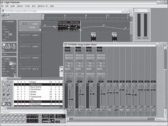
© Apple Inc.
Figure 1.3 Logic Pro X, the most recent version of Logic, running on Mac OS X. You can see that even with the integrated features of the main window, the two versions of Logic still resemble each other.
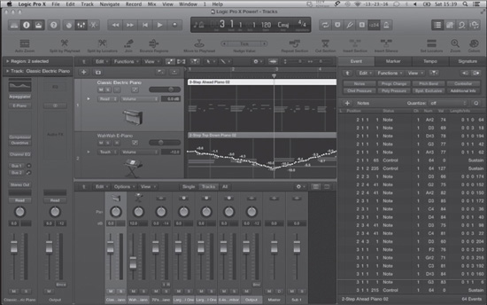
© Apple Inc.
The MIDI protocol specifies that every MIDI-compliant device that can both send and receive MIDI information must have a MIDI IN port to accept MIDI data, a MIDI OUT port to transmit MIDI data, and optionally a MIDI THRU port for transferring data between other MIDI devices. When you connect the MIDI OUT port of one device to the MIDI IN port of another device, the first device enables you to press a key, turn a dial, engage a control message, and so on, and the second device will receive the data.
In addition to providing hardware specifications that allow devices to send and receive MIDI, the MIDI protocol also defines how to pass data from one device to another. MIDI is a serial protocol, meaning that MIDI information is sent one event (or MIDI message) at a time. That may sound inefficient, but the speed of MIDI transfer is 31,250 bits per second (bps), where bit stands for binary digit. Because each MIDI message uses 10 bits (eight for the information, two for error correction), the MIDI protocol can send 3,906 bytes of data every second (31,250 divided by 8 bits to convert bits to bytes). Because one MIDI note can take up to 6 bytes, the protocol enables a device to play approximately 500 MIDI notes per second. This might seem like a lot of notes, but as soon as you add a couple five-note chords in a single 10-millisecond span of time, with multiple MIDI control messages, you might very well start seeing some compromised timing. That’s why for the most demanding MIDI productions, there are MIDI time-stamping features on many MIDI interfaces to improve MIDI timing even further.
Even if you have no external MIDI hardware, MIDI is still the protocol that Logic uses for internal playback and automation of virtual instruments, so it’s still useful to understand some basics about MIDI.
What MIDI Really Transmits
The most important thing to understand is that MIDI doesn’t transmit any sound at all. It transmits only data. In other words, when you record digital audio, you’re recording an actual file of digital information that will play back as sound. When you record MIDI data, you’ll then need some sort of device—a synthesizer, drum machine, sampler, or software instrument—to actually hear that MIDI information. MIDI data can transmit the following:
![]() Performance events, such as when you play and release notes, and their velocities.
Performance events, such as when you play and release notes, and their velocities.
![]() The pressure with which you press the keys as you play (known as aftertouch).
The pressure with which you press the keys as you play (known as aftertouch).
![]() Information from MIDI controller wheels, knobs, pedal controls, ribbon controllers, pitchbend controllers, and so on that send parameters that affect performance.
Information from MIDI controller wheels, knobs, pedal controls, ribbon controllers, pitchbend controllers, and so on that send parameters that affect performance.
![]() Channel settings. Each MIDI cable can support up to 16 channels, so each device can operate as 16 devices in one. Devices that can support multiple MIDI channels are called multitimbral devices.
Channel settings. Each MIDI cable can support up to 16 channels, so each device can operate as 16 devices in one. Devices that can support multiple MIDI channels are called multitimbral devices.
![]() Synchronization information, so that all time-sensitive instruments or functions on various devices can operate from the same master clock and play in sync with each other.
Synchronization information, so that all time-sensitive instruments or functions on various devices can operate from the same master clock and play in sync with each other.
![]() Program changes and sound-bank selections.
Program changes and sound-bank selections.
![]() MIDI Time Code (MTC), which allows MIDI devices to lock to devices that use Society of Motion Picture and Television Engineers (SMPTE)–format time code by translating SMPTE into something that the MIDI device can understand.
MIDI Time Code (MTC), which allows MIDI devices to lock to devices that use Society of Motion Picture and Television Engineers (SMPTE)–format time code by translating SMPTE into something that the MIDI device can understand.
![]() System Exclusive messages, which are unique messages that can alter parameters and control of one specific MIDI device. Most MIDI synthesizers and some multitrack recorders offer unique System Exclusive commands.
System Exclusive messages, which are unique messages that can alter parameters and control of one specific MIDI device. Most MIDI synthesizers and some multitrack recorders offer unique System Exclusive commands.
MIDI Connections and Signal Flow
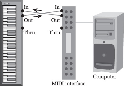
As described previously, connecting MIDI devices couldn’t be simpler. The most basic type of MIDI connection, in which the MIDI OUT jack of one MIDI device is connected to the MIDI IN jack of another MIDI device, allows the first unit to send MIDI to the second unit, as shown in Figure 1.4.
Note that this type of connection does not allow for two-way communication, only one-way communication. This type of connection is most common when connecting a MIDI controller, which is a MIDI device that does not itself produce sounds (and doesn’t receive MIDI), but can send MIDI to other devices, such as to a computer MIDI interface or another MIDI device.
An example of another simple but more dynamic MIDI connection is to connect both the MIDI IN and MIDI OUT of one device to the MIDI OUT and MIDI IN of another device, as shown in Figure 1.5.
Figure 1.4 A basic MIDI connection between a MIDI OUT jack on a MIDI device and a MIDI IN jack on a MIDI interface, which is then connected to the computer. This type of MIDI connection allows the MIDI device to control MIDI software in the computer.
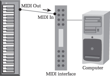
© Cengage Learning.
Figure 1.5 A new MIDI connection has been added to the system seen in Figure 1.4. The MIDI IN on the MIDI device has been connected to the MIDI OUT on the MIDI interface, allowing the MIDI software on the computer to control the MIDI device.
© Cengage Learning.
This enables two-way communication between MIDI devices, so each is capable of both sending and receiving data from the other. This is the most common form of routing between two devices capable of sending and receiving MIDI information, such as two synthesizers, or a computer and a synthesizer.
CAUTION: When making connections like this, be sure both units have MIDI THRU and/or local control turned off, or else you might end up with a MIDI feedback loop. In a MIDI feedback loop, one unit sends a command to the other, which then sends the command back to the first unit, and on and on endlessly.
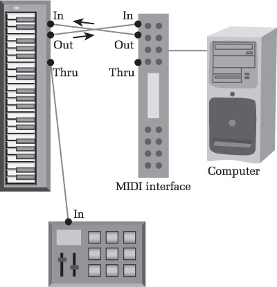
A final example of a basic MIDI connection illustrates how three MIDI devices might be connected via a MIDI THRU port. The MIDI OUT of the first device is connected to the MIDI IN of the second device, the MIDI OUT of the second device is connected to the MIDI IN of the first device, and the MIDI THRU of the second device is connected to the MIDI IN of the third device (see Figure 1.6).
In Figure 1.6, complete two-way communication between the first two devices is possible, and the first device (and often the second device) can also send MIDI information to the third device. Such connections are often used when a third MIDI device, such as a drum machine, is not being used to issue any MIDI messages, but only to receive them from the rest of the MIDI setup.
At this point, you should have a good understanding of what MIDI is and the importance of getting MIDI information into Logic. Because Logic can both send and receive MIDI, you will probably want a MIDI interface—a universal serial bus (USB) device that accepts MIDI from MIDI devices and sends it into Logic—that has at least as many MIDI IN and MIDI OUT ports as you have MIDI devices. This will be discussed later in this chapter, in the section “A Brief Primer on Hardware.”
Figure 1.6 A new MIDI connection has been added to the system seen in Figure 1.5. The MIDI THRU on the original MIDI device has been connected to the MIDI IN on another MIDI device. This allows the MIDI software on the computer to control the second MIDI device.
© Cengage Learning.
A Brief Overview of Digital Audio
These days, recording digital audio is perhaps the most popular use of sequencers such as Logic Pro. In fact, the popular term to describe a computer used as the hub of a music production system is a digital audio workstation (DAW). So what is digital audio? How does it differ from analog audio? Why is it important?
While a complete technical reference on the details of digital audio would result in a book almost as large as this one, it is important to know at least enough about the fundamentals of digital audio to be able to make a good recording. The following subsections should give you just enough of a background to get the most out of your audio recordings.
The Differences Between Analog and Digital Sound
We hear sound when our eardrums vibrate. If you read that carefully, you will realize that it did not say that we hear sound whenever some object vibrates. Many objects vibrate outside our ability to hear them (think of dog whistles or ultra-low subfrequencies). Our ears are theoretically capable of registering vibrations (also called cycles) that oscillate between 20 and 20,000 times a second. This is called the frequency—which is pretty logical when you think about it, because the term refers to the frequency of vibrations per second. Theoretically, then, humans can hear frequencies from 20 Hz to 20 kHz. (The measurement Hertz, or Hz, is named after Henry Hertz, who in 1888 developed the theory of the relationship between frequency and cycles.) In practice, hardly any adult’s hearing reaches that theoretical maximum because people lose the ability to hear certain frequencies (high-pitched ones in particular) as they age, are subjected to loud noises, and so on.
If the frequency of vibration is slow (say, 60 vibrations per second, or 60 Hz), we perceive a low note. If the frequency of the vibration is fast (say, 6,000 vibrations per second, or 6 kHz), we would perceive a high note. If the vibrations are gentle, barely moving our eardrums, we perceive the sound as soft. The loudness and softness of the sound is called the amplitude, because the term refers to the volume, or amplification, of the sound. Thus we can graph sound as you see in Figure 1.7.
In the graph in Figure 1.7, the frequency is the distance between the oscillations of the waveform, and the amplitude is the height of the waveform. Most sounds we hear in the real world are complex ones that have more than a single frequency in them, as in the graph in Figure 1.8.
Figure 1.7 A graphical representation of a simple sound wave. This particular kind of even, smooth sound wave is known as a sine wave.
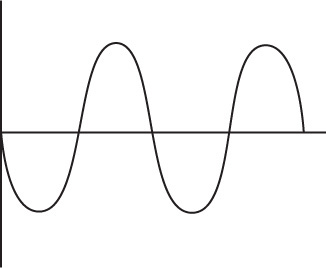
© Cengage Learning.
Figure 1.8 A more complex sound wave than the one seen in Figure 1.7. This example has more than a single tone in it, and not every frequency is being heard at the same volume (amplitude).
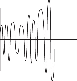
© Cengage Learning.
Now that you understand a little about sound waves, let’s tie it into recording. One way to record sound is to make an exact replica of the original waveform on some other media. For example, you might carve an image of the waveform onto a vinyl surface or imprint the waveform on magnetic tape. In these cases, you have recorded an actual copy of the original sound wave. Now you just need a machine to amplify the sound so it’s loud enough to listen to (or to rattle the windows, if that’s your style). Because this type of recording results in a continuous waveform, it’s called analog recording. Analog refers to any signal that is represented by a continuous, unbroken waveform.
Because a computer works using mathematical codes instead of actual pictures of objects, to use a computer for recording audio, we need to translate the actual analog signal into math. Luckily, sound can also be represented digitally—meaning by use of digits, or numbers. Basically, complex mathematical analysis has proven that if we sample a waveform twice in each cycle, or period, and record its variation in sound, we can reproduce the waveform. Now, each period is a full cycle, or vibration. That means if we wanted to reproduce a 60-Hz sound, which is 60 cycles, we’d need to take at least 120 samples. From this, you can see that if you want to capture the full range of human hearing—20 kHz, or 20,000 cycles—you have to take at least 40,000 samples.
What’s Meant by Sampling Frequency and Bit Depth
From the preceding, we understand that we have to represent the sound wave as numbers to store it in the computer, and that by storing two samples per cycle we can represent that cycle. You’ve probably noticed that every recording interface and program that handles digital audio refers to sample rate and bit depth. I’ll explain what these terms mean and how they affect your recording.
As explained, it takes two samples per cycle to represent each cycle accurately. It follows that the total number of samples taken of a waveform determines the maximum frequency that will be recorded. This is called the sampling frequency or sampling rate. For example, the sampling rate of the compact disc is fixed at 44.1 kHz, or 44,100 samples per second. It’s a few thousand samples more than the minimum needed to represent the highest-frequency sound wave that humans can hear.
You’ve probably noticed that many audio interfaces today boast sampling rates of 96 kHz or even 192 kHz (kHz is short for kilohertz, or 1,000 Hz). That means these devices can represent sounds up to 48 kHz and 96 kHz. The obvious question is, why bother? We can only hear up to a theoretical 20 kHz anyway, right? Of course, it’s not quite that simple. Although we may not be able to distinguish sounds accurately above a certain frequency, every sound also contains additional overtones, harmonics, spatial cues, and so on. These features enrich the sound, help us place it in space, and so on. When our sampling rate is too low to represent such features, they are simply discarded and lost forever. We may not consciously notice these “ultrasonic” frequencies when we listen to recordings, but many audiophiles and sound engineers believe that they contribute to a far more realistic listening experience.
That explains sampling rates, but what about bit depth? Remember, the sound wave has two components: the frequency and the amplitude. The mathematical representation of the amplitude at a particular instant in a particular cycle is stored in bits. A computer cannot interpolate information between the amplitudes you have stored—it only knows what the amplitude at a given instant in the cycle is if the amplitude is stored in a bit. The more bits used to store the amplitude per cycle, the more accurate the representation.
Finally, here is a loose—but good—analogy to give you a basic understanding of analog versus digital audio, sampling rate, and bit depth. If you make an analog recording, you are left with an actual copy of the audio waveform imprinted onto your media. If you make a digital recording, you are instead taking “snapshots” of the waveform and then attempting to re-create the waveform from those snapshots. Your sampling rate would be the number of snapshots you take every second, and your bit depth would represent the focus and color quality of each snapshot. As you can see, the higher the sampling rate and bit depth, the closer your snapshots will get to the actual sound wave, as follows in Figure 1.9.
Figure 1.9 The higher the sampling rate and bit depth, the closer your snapshots will get to the actual sound wave.
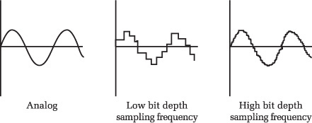
© Cengage Learning.
In analog recording, you record an accurate representation of the source, in this case a sine wave. In digital recording, the sample rate and bit depth directly influence the accuracy of the recording. With higher sample rates and bit depths, you can achieve a more accurate digital representation of the source than with lower sample rates and bit depths.
You should also keep in mind that as your bit depths and sampling rates increase, so do the processor, memory, and hard-drive requirements. The larger the bit depth and sample rate, the more CPU is required to process it, the more memory the audio requires during processing, and the more space on your hard disk the audio will require.
It is beyond the scope of this book to give comprehensive position papers on the merits of analog versus digital audio. The important things to remember are that any audio waveform that gets into your computer will be digital audio, and you need to be aware of sampling frequency and bit depth to get the most out of your hardware and out of Logic.
Audio and MIDI in Logic Pro
It’s time to relate all of this to what it means for Logic. In its simplest description, Logic is a software MIDI and digital audio recorder. In other words, if you connect your MIDI devices to your computer, connect your audio devices to your computer, and then activate the Record function in Logic, you will record your audio and MIDI into Logic. If you then activate the Play function, you will hear the MIDI and audio you’ve just recorded. So far, this should be familiar to pretty much anyone who has ever used a DVR to record and watch their favorite shows.
For Logic to be able to record MIDI and digital audio information, you need a way to capture that information into the computer, and then a way to transfer that information out of the computer when you activate playback. In the case of audio, you capture and transfer this information through your audio interface. In the case of MIDI, you handle all of this with your MIDI interface.
Unlike a DVR, which requires little more setting up than telling it what channel to record at what time, Logic is famous (perhaps infamous) for the depth and breadth of setup and configuration options it offers. Logic Pro X’s processes are streamlined so that you can configure your setup on a basic level very quickly, while still allowing the incredible amount of flexibility for which it is famous.
A Brief Primer on Hardware
It is beyond the scope of this book to give you a complete buyer’s guide on computer hardware. It is also relatively pointless, because new products are introduced almost daily. But it is important to touch a little bit on the basic kinds of hardware you’ll need to get the most out of Logic.
We’ll assume that you already have any musical instruments or MIDI controller devices you will be using. If you already have your computer hardware as well and are ready to set it up, feel free to skip to Chapter 2, “A Quick Tour of Logic Pro.”
How Fast Does Your Computer Need to Be?
The simple answer to this question is as fast as possible! The more detailed answer is that it depends on what sort of music production you expect to be doing and what your expectations are.
Apple’s stated minimum requirements are for an Intel Macintosh computer. Apple goes on to recommend the following:
![]() A minimum of 4 GB of random access memory (RAM)
A minimum of 4 GB of random access memory (RAM)
![]() A display with a resolution of 1,280×768
A display with a resolution of 1,280×768
![]() The Mac OS X 10.8.4 or later operating system
The Mac OS X 10.8.4 or later operating system
![]() 5 GB minimum drive space
5 GB minimum drive space
Logic also offers 35 GB of extra content—samples and loops—via an in-app download. The extra content is of a high enough level of quality that I would recommend making space on your drive for it.
If you intend to run a sizable number of effects and software synthesizers, your processor and RAM requirements will increase. Logic does have a Freeze function and Bounce in Place functions that can help conserve CPU power, but the more processor power and the more RAM you have, the better. (I’d recommend at least 8 GB of RAM if your system can handle it.)
If your computer is older and you are thinking of pushing the minimum, be warned: Slow computers not only have slower CPUs, but also usually have slower motherboards, hard drives, RAM, and so on. When you ask your computer basically to replace an entire building full of mixing desks, tape machines, effects units, and MIDI synthesizers, you’re asking a lot. Although Logic Pro X is a very efficient program, it contains some very powerful, industry-leading tools that not only can inspire you and benefit your productions, but can bring even more recent computers to their knees fairly quickly. Keep that in mind.
My recommendation is that you get the fastest laptop or desktop Macintosh you can afford and load it with as much RAM as you can. You won’t be sorry!
Different Types of Storage Drives
Traditionally, storage drives operate on the principle of a set of needles reading and writing data on magnetic platters that spin around incredibly fast. This type of platter hard drive (HDD) has been the industry standard for decades. The differences among the various types of HDDs are mainly in how fast these platters spin and what mechanism they use to connect to the rest of the computer. In recent years, solid-state drives (SSDs), basically large-capacity flash drives, have become more practical financially. SSDs have no moving parts and therefore offer the potential for much higher performance than HDD technology.
Storage drives use two mainstream transfer mechanisms to communicate with the host computer: Advanced Technology Attachment (ATA) and Small Computer Systems Interface (SCSI). Both formats have different performance subcategories, such as SATA, eSATA, ATA/66 or ATA/100, and SCSI-2 or SCSI-3. SCSI drives have higher top speeds, usually require an additional PCI Express expander or ExpressCard that supports the SCSI protocol (although some newer Macs support the USB Attached SCSI protocol), and generally cost more than similar-sized ATA drives. ATA is inexpensive, ubiquitous, and supported internally by every desktop and notebook system designed since 1998. eSATA is an external SATA standard that offers transfer rates that match that of internal SATA drives.
Recording audio files to an HDD can be a very disk-intensive task, and a faster hard drive can record and play back more simultaneous tracks. Most desktop and external hard drives these days spin at 7,200 RPM, which is fast enough to reliably handle songs with around 64 to 72 audio tracks—more than enough for most people. If you have a 7,200-RPM hard drive and you still need more tracks, you can either record audio to two different storage drives or get a faster drive. These days, hard drives running up to 15,000 RPM are available, although they are expensive and almost always require SCSI.
SSDs offer a few advantages over HDDs. First, because they have no moving parts, SSDs are silent in operation. If you work with your Mac Pro in the room with you, or with a laptop or iMac, eliminating any bit of extra computer noise is helpful. Second, SSDs have much faster read and write speeds. If a drive doesn’t have to physically search for data or space to place data, it can work much more quickly and efficiently. Third, newer SSDs have longer projected life spans than HDDs. SSDs do have one major drawback: cost. For example, as of this writing, SSDs approaching 1 TB of storage cost $600 and more for just the drive, while 3-TB 7,200-RPM drives in external enclosures can be found for around $100.
If you are using a laptop with an internal HDD, it could spin at 5,400 RPM or 7,200 RPM. The MacBook Air series uses internal SSDs, and SSDs are an option you can configure when purchasing a new MacBook Pro, iMac, or Mac Pro. If you already have a MacBook Pro, many of the more recent ones allow easy access to the storage drive, enabling you to easily upgrade the capacity, speed, or type of drive installed. For high-performance mobile use, you should consider using an external HDD that runs at 7,200 RPM as your audio drive, particularly if you’re running a slower internal drive. Several external HDDs are available in USB, FireWire, eSATA, or Thunderbolt enclosures that offer plug-and-play connectivity to all notebook computers with those ports. External SSDs are available, but their cost is, of course, very high at this time.
If your laptop doesn’t have enough USB or FireWire ports but supports the use of an ExpressCard, you can buy an ExpressCard that will allow you to connect more USB or FireWire devices. You can also find eSATA ExpressCards that will allow you to use eSATA drives with your laptop. For Thunderbolt-equipped computers, you can buy hubs that offer USB, FireWire, Ethernet, and extra Thunderbolt ports, allowing you to connect several storage drives and peripherals to your computer.
Do You Need a Separate Storage Drive for Audio Files?
In general, the more a storage drive has to do, the less performance it has left over for audio. In other words, if your drive needs to read system files as well as audio files, it needs to divide its attention. If you have a drive devoted to nothing but recording audio files, that drive could dedicate 100 percent of its performance to audio-related tasks.
Clearly, having a separate drive for audio seems advantageous, but is it absolutely necessary? The answer to this depends on how audio-intensive your projects are. Even a slower hard disk should be able to run both system software and approximately 16–24 tracks of audio. If your needs are modest, you really shouldn’t need a separate storage drive for your audio tracks. On the other hand, professional studios that need to record anything from solo singers all the way to full orchestras often have entire banks of storage drives. If you regularly work with songs in excess of 24 tracks or you can easily afford it, you should go ahead and buy a separate drive for audio files.
Even if you don’t choose to buy extra drives for audio, I can’t stress enough the importance of having at least one backup drive for your system. Regardless of the type of drive you use, drives do fail—typically in spectacular fashion at the worst possible moment. Back up, back up, back up.
MIDI Interfaces
Earlier, the section “A Brief Overview of MIDI” concluded by mentioning the MIDI interface. This device has the same MIDI IN and MIDI OUT ports that your MIDI hardware does and connects to your computer via USB to send that MIDI information from your external units into Logic, and vice versa. If you want Logic to be able to communicate with MIDI devices outside the computer, you need a MIDI interface.
So what size interface do you need? That depends completely on how many MIDI devices you have. Do you have only one controller keyboard? If so, then you just need a simple MIDI interface with one MIDI IN and one MIDI OUT port. It’s also common for modern MIDI controllers to have their own USB MIDI connectors. If your needs are modest enough, your audio interface may already have all the MIDI ports you need. (See the following section, “Audio Interfaces.”) Do you have a full MIDI studio and need 12 MIDI ports? In that case, you need to buy multiple MIDI interfaces of the largest size you can find (usually eight MIDI IN and eight MIDI OUT ports). Also think about whether you plan to expand your MIDI hardware over time. If you do, you might want to get a MIDI interface with more ports than you currently need.
Another thing to consider is whether your MIDI interface needs any professional synchronization features. Some of the more professional interfaces include a lot of video and hardware synchronization options that you might need if you do a lot of sound-to-picture work. Also, many of the larger interfaces include time-stamping functionality, which allows them to stamp the exact time that a MIDI event should occur as part of the MIDI message. Time stamping doesn’t have a noticeable effect for small numbers of MIDI devices, but it can make a world of difference with MIDI studios containing large amounts of external hardware.
Finally, keep in mind that many different manufacturers make MIDI interfaces, and these interfaces are all equally compatible with Logic. As long as your interface has a USB connector and drivers for your Mac OS X, it should do the job.
Audio Interfaces
Because there are so many audio interfaces on the market, choosing one might seem daunting. Here are a few tips to help you with your selection.
First, consider how many audio channels you intend to record at one time. Do you see yourself recording a rock band or an entire symphony at once? If so, you will want to investigate those audio interfaces that enable users to daisy-chain more than one interface, so you can expand your system as your recording needs grow. Some systems today not only enable users to record 24 or more channels at once, but to connect two or three such boxes for a truly impressive audio recording system. On the other hand, do you see yourself recording only yourself or one stereo instrument at a time? If so, then a single interface with fewer inputs will do.
Next, consider how you would prefer or need your audio interface to connect to your computer. Are you using a laptop or an iMac? If so, you probably want an interface that connects to the computer via USB, FireWire, or Thunderbolt. All Intel Macintosh laptops and iMacs have USB connections. The availability of FireWire or Thunderbolt will depend on the age of your machine—for example, the newer MacBooks offer Thunderbolt and USB, but you can still use FireWire via a Thunderbolt-to-FireWire adapter. Older MacBooks are incompatible with Thunderbolt, but most offer FireWire. Some older MacBook Pros also allow you to select an ExpressCard format interface. If you have a Mac Pro, you might also prefer a USB, FireWire, or Thunderbolt interface, depending on what connections are available on your machine, because those interfaces don’t require you to open up your machine and install anything. If you don’t mind installing hardware in your older Mac Pro, you can choose an audio interface that is a Peripheral Component Interface Express (PCI Express) card. PCI Express options are usually more expandable and less expensive than USB, FireWire, and ExpressCard interfaces, but are more difficult to install. The newest Mac Pros no longer support internal expansion, but there are external Thunderbolt-based PCI Express expansion chassis on the market, which will also work with Thunderbolt-equipped MacBooks and iMacs.
You need to consider the sampling frequency and bit depth at which you want to record. Compact discs are standardized at 16 bits, with a sampling frequency of 44.1 kHz. Every audio interface available today can record at least at this level of fidelity. Do you want to be able to record at 24 bits, which is the industry standard for producing music? Do you want to be able to record at higher sampling frequencies, such as the 96 kHz that DVDs can use? All these decisions influence what kind of audio interface will fit your needs. Because the higher bit depths and sample rates capture a more accurate “picture” of the sound, as explained, you might want to record and process your audio at higher bit rates than your final format if you have the computer power to do so.
Finally, you should consider whether you want your audio interface to have additional features. For example, some audio interfaces have MIDI control surfaces and/or MIDI interfaces as part of a package. Does that appeal to you, or would you prefer to fill those areas with other devices?
Now that I’ve introduced Logic, some of its basic concepts, and the hardware you’ll need, it’s time to take “A Quick Tour of Logic Pro.”