Chapter 2

Passive Components

Conductors

It is easy to assume, when wrestling with electronic design, that the active devices will cause most of the trouble. This, like so much in electronics, is subject to Gershwin’s law; it ain’t necessarily so. Passive components cannot be assumed to be perfect, and while their shortcomings are rarely discussed in polite company, they are all too real. In this chapter I have tried to avoid repeating basic stuff that can be found in many places, to allow room for information that goes deeper.

Normal metallic conductors, such as copper wire, show perfect linearity for our purposes, and as far as I am aware, for everybody’s purposes. Ohm’s law was founded on metallic conductors, after all, not resistors, which did not exist as we know them at the time. George Simon Ohm published a pamphlet in 1827 titled, “The Galvanic Circuit Investigated Mathematically” while he was a professor of mathematics in Cologne. His work was not warmly received, except by a perceptive few; the Prussian minister of education pronounced that “a professor who preached such heresies was unworthy to teach science”. This is the sort of thing that happens when politicians try to involve themselves in science, and in that respect we have progressed little since then.

Although the linearity is generally effectively ideal, metallic conductors will not be perfectly linear in some circumstances. Poorly made connections between oxidised or otherwise contaminated metal parts are capable of generating harmonic distortion at the level of several percent, but this is a property of the contact interface rather than the bulk material and usually means that the connection is about to fail altogether. A more subtle danger is that of magnetic conductors—the soft iron in relay frames causes easily detectable distortion at power amplifier current levels.

From time to time some of the dimmer audio commentators speculate that metallic conductors are actually a kind of “sea of micro-diodes”, and that nonlinearity can be found if the test signal levels are made small enough. This is both categorically untrue and physically impossible. There is no threshold effect for metallic conduction. I have myself added to the mountain of evidence on this, by measuring distortion at very low signal levels.[1] Renardsen has some more information online.[2]

One account of distortion in a metal, in this case a binary alloy, is known to me. Takahisa’s test[3] subjected a very thin (less than 0.001 mm) nickel-chrome alloy film to 250 volts at 10 kHz. This is the kind of film used in metal film resistors. The distortion measured was only 0.00004% of third harmonic. Other harmonics were found at a much lower level. All of these results indicate that Takahisa was measuring thermal distortion, caused by changes in resistance due to cyclic heating by the test signal and correspond with the results for actual metal film resistors—see later in this chapter. Takahisa would have found much higher distortion at lower frequencies such as 10 Hz. I would emphasise that these results actually relate only to the thin films found in resistors and not wiring or cables, where the metal thickness is far greater and cyclic heating utterly negligible.

Copper and Other Conductive Elements

Copper is the preferred metal for conducting electricity in almost all circumstances. It has the lowest resistance of any metal but silver, is reasonably resistant to corrosion, and can be made mechanically strong; it’s wonderful stuff. Being a heavy metal, it is unfortunately not that common in the earth’s crust, and so is expensive compared with iron and steel. It is however cheap compared with silver. The price of metals varies all the time due to changing economic and political factors, but at the time of writing silver was 100 times more expensive than copper by weight. Given the same cross-section of conductor, the use of silver would only reduce the resistance of a circuit by 5%. Despite this, silver connection wire has been used in some very expensive hi-fi amplifiers; output impedance-matching transformers wound with silver wire are not unknown in valve amplifiers. Since the technical advantages are usually negligible, such equipment is marketed on the basis of indefinable subjective improvements. The only exception is the moving-coil step-up transformer, where the use of silver in the primary winding might give a measurable reduction in Johnson noise.

Table 2.1 gives the resistivity of the commonly used conductors, plus some insulators to give it perspective. The difference between copper and quartz is of the order of 10 to the 25, an enormous range that is not found in many other physical properties.

Table 2.1 Properties of conductors and nonconductors

Material	Resistivity ρ (Ω − m)	Temperature coefficient per degree C	Electrical usage
Silver	1.59 × 10−8	0.0061	conductors
Copper	1.72 × 10−8	0.0068	conductors
Gold	2.2 × 10−8	0.0041	inert coatings
Aluminium	2.65 × 10−8	0.00429	conductors
Tungsten	5.6 × 10−8	0.0045	lamp filaments
Iron	9.71 × 10−8	0.00651	barreters*
Platinum	10.6 × 10−8	0.003927	electrodes
Tin	11.0 × 10−8	0.0042	coatings
Mild steel	15 × 10−8	0.0066	busbars
Solder (60:40 tin/lead)	15 × 10−8	0.006	soldering
Lead	22 × 10−8	0.0039	storage batteries
Manganin (Cu,Mn,Ni)**	48.2 × 10−8	0.000002	resistances
Constantan (Cu,Ni)**	49–52 × 10−8	±0.00002	resistances
Mercury	98 × 10−8	0.0009	relays
Nichrome (Ni,Fe,Cr alloy)	100 × 10−8	0.0004	heating elements
Carbon (as graphite)	3–60 × 10−5	−0.0005	brushes
Glass	1–10000 × 109	…	insulators
Fused quartz	More than 1018	…	insulators

^* A barreter is an incredibly obsolete device consisting of thin iron wire in an evacuated glass envelope. It was typically used for current regulation of the heaters of RF oscillator valves, to improve frequency stability.

^** Constantan and Manganin are resistance alloys with moderate resistivity and a low temperature coefficient. Constanan is preferred as it has a flatter resistance/temperature curve and its corrosion resistance is better.

There are several reasonably conductive metals that are lighter than copper, but their higher resistivity means they require larger cross-sections to carry the same current, so copper is always used when space is limited, as in electric motors, solenoids, etc. However, when size is not the primary constraint, the economics work out differently. The largest use of noncopper conductors is probably in the transmission line cables that are strung between pylons. Here minimal weight is more important than minimal diameter, so the cables have a central steel core for strength, surrounded by aluminium conductors.

It is clear that simply spending more money does not automatically bring you a better conductor; gold is a somewhat poorer conductor than copper, and platinum, which is even more expensive, is worse by a factor of six. Another interesting feature of this table is the relatively high resistance of mercury, nearly 60 times that of copper. This often comes as a surprise; people seem to assume that a metal of such high density must be very conductive, but it is not so. There are many reasons for not using mercury-filled hoses as loudspeaker cables, and their conductive inefficiency is just one. The cost and the insidiously poisonous nature of the metal are two more. Nonetheless … it is reported that the Hitachi Cable company has experimented with speaker cables made from polythene tubes filled with mercury. There appear to have been no plans to put such a product on the market. Restriction of Hazardous Substances (RoHS) compliance might be a problem.

We also see that the resistivity of solder is high compared with that of copper—nine times higher if you compare copper with the 60/40 tin/lead solder. This is unlikely to be a problem because the thickness of solder the current passes through in a typical joint is very small. There are many formulations of lead-free solder, with varying resistivities, but all are high compared with copper.

The Metallurgy of Copper

Copper is a good conductor because the outermost electrons of its atoms have a large mean free path between collisions. The electrical resistivity of a metal is inversely related to this electron mean free path, which in the case of copper is approximately 100 atomic spacings.

Copper is normally used as a very dilute alloy known as electrolytic tough pitch (ETP) copper, which consists of very high purity metal alloyed with oxygen in the range of 100 to 650 ppm. In view of the wide exposure that the concept of oxygen-free copper has had in the audio business, it is worth underlining that the oxygen is deliberately alloyed with the copper to act as a scavenger for dissolved hydrogen and sulphur, which become water and sulphur dioxide. Microscopic bubbles form in the mass of metal but are completely eliminated during hot rolling. The main use of oxygen-free copper is in conductors exposed to a hydrogen atmosphere at high temperatures. ETP copper is susceptible to hydrogen embrittlement in these circumstances, which arise in the hydrogen-cooled alternators in power stations.

Gold and Its Uses

As stated earlier, gold has a higher resistivity than copper, and there is no incentive to use it as the bulk metal of conductors, not least because of its high cost. However it is very useful as a thin coating on contacts because it is almost immune to corrosion, though it is chemically attacked by fluorine and chlorine. (If there is a significant amount of either gas in the air then your medical problems will be more pressing than your electrical ones.) Other electrical components are sometimes gold-plated simply because the appearance is attractive. A carat (or karat) is a 1/24 part, so 24-carat gold is the pure element, while 18-carat gold contains only 75% of the pure metal. Eighteen-carat gold is the sort usually used for jewellery because it retains the chemical inertness of pure gold but is much harder and more durable; the usual alloying elements are copper and silver.

Eighteen-carat gold is widely used in jewellery and does not tarnish, so it is initially puzzling to find that some electronic parts plated with it have a protective transparent coating which the manufacturer claims to be essential to prevent blackening. The answer is that if gold is plated directly onto copper, the copper diffuses through the gold and tarnishes on its surface. The standard way of preventing this is to plate a layer of nickel onto the copper to prevent diffusion, then plate on the gold. I have examined some transparent-coated gold-plated parts and found no nickel layer; presumably the manufacturer finds the transparent coating is cheaper than another plating process to deposit the nickel. However, it does not look as good as bare gold.

Cable and Wiring Resistance

Electrical cable is very often specified by its cross- sectional area and current-carrying capacity, and the resistance per metre is seldom quoted. This can however be a very important parameter for assessing permissible voltage drops and for predicting the crosstalk that will be introduced between two signals when they unavoidably share a common ground conductor. Given the resistivity of copper from Table 2.1, the resistance R of L metres of cable is simply:

$R=\frac{resistivity\cdot L}{area}$

2.1

Note that the area, which is usually quoted in catalogues in square millimetres, must be expressed here in square metres to match up with the units of resistivity and length. Thus 5 metres of cable with a cross-sectional area of 1.5 mm² will have a resistance of:

This gives the resistance of our stretch of cable, and it is then simple to treat this as part of a potential divider to calculate the voltage drop down its length.

PCB Track Resistance

It is also useful to be able to calculate the resistance of a PCB track for the same reasons. This is slightly less straightforward to do; given the smorgasbord of units that are in use in PCB technology, determining the cross-sectional area of the track can present some difficulty.

In the USA and the UK, and probably elsewhere, there is inevitably a mix of metric and imperial units on PCBs, as many important components come in dual-in-line packages which are derived from an inch grid; track widths and lengths are therefore very often in thousandths of an inch, universally (in the UK at least) referred to as “thou”. Conversely, the PCB dimensions and fixing-hole locations will almost certainly be metric because they interface with a world of metal fabrication and mechanical CAD that (except in the USA) went metric many years ago. Add to this the UK practice of quoting copper thickness in ounces (the weight of a square foot of copper foil) and all the ingredients for dimensional confusion are in place.

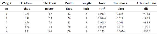
Standard PCB copper foil is known as one-ounce copper, having a thickness of 1.4 thou (= 35 microns). Two-ounce copper is naturally twice as thick; the extra cost of specifying it is small, typically around 5% of the total PCB cost, and this is a very simple way of halving track resistance. It can of course be applied very easily to an existing design without any fear of messing up a satisfactory layout. Four-ounce copper can also be obtained but is more rarely used and is therefore much more expensive. If heavier copper than two-ounce is required, the normal technique is to plate two-ounce up to three-ounce copper. The extra cost of this is surprisingly small, in the region of 10% to 15%.

Given the copper thickness, multiplying by track width gives the cross-sectional area. Since resistivity is always in metric units, it is best to convert to metric at this point, so Table 2.2 gives area in square millimetres. This is then multiplied by the resistivity, not forgetting to convert the area to metres for consistency. This gives the “resistance” column in the table, and it is then simple to treat this as part of a potential divider to calculate the usually unwanted voltage across the track.

For example, if the track in question is the ground return from a 1 kΩ load on an opamp, the load is the top half of a potential divider while the track is the bottom half, and a quick calculation gives the fraction of the input voltage found along the track. This is expressed in the last column of Table 2.2 as attenuation in dB. This shows clearly that circuit sections should not have common return tracks, or the interchannel crosstalk will be poor.

It is very clear from this table that relying on thicker copper on your PCB as means of reducing path resistance is not very effective. In some situations it may be the only recourse, but in many cases a path of much lower resistance can be made by using 32/02 cable soldered between the two relevant points on the PCB.

PCB tracks have a limited current capability because excessive resistive heating will break down the adhesive holding the copper to the board substrate and ultimately melt the copper. This is normally only a problem in power amplifiers and power supplies. It is useful to assess if you are likely to have problems before committing to a PCB design, and Table 2.3, based on MIL-standard 275, gives some guidance.

Note that Table 2.3 applies to tracks on the PCB surface only. Internal tracks in a multi-layer PCB experience much less cooling and need to be about three times as thick for the same temperature rise. This factor depends on laminate thickness and so on, and you need to consult your PCB vendor.

Traditionally, overheated tracks could be detected visually because the solder mask on top of them would discolour to brown. I am not sure if this still applies with modern solder mask materials, as in recent years I have been quite successful in avoiding overheated tracking.

PCB Track-to-Track Crosstalk

The previous section described how to evaluate the amount of crosstalk that can arise because of shared track resistances. Another crosstalk mechanism is caused by capacitance between PCB tracks. This is not very susceptible to calculation, so I did the following experiment to put some figures to the problem.

Figure 2.1 shows the setup; four parallel conductors 1.9 inches long on a standard piece of 0.1 inch pitch prototype board were used as test tracks. These are perhaps rather wider than the average PCB track, but one must start somewhere. The test signal was applied to track A, and track C was connected to a virtual-earth summing amplifier A1.

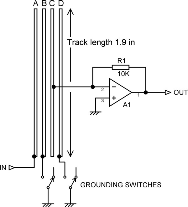
The tracks B and D were initially left floating. The results are shown as Trace 1 in Figure 2.2; the coupling at 10 kHz is −65 dB, which is worryingly high for two tracks 0.2 inch apart. Note that the crosstalk increases steadily at 6 dB per octave, as it results from a very small capacitance driving into what is effectively a short circuit.

It has often been said that running a grounded screening track between two tracks that are susceptible to crosstalk has a beneficial effect, but how much good does it really do? Grounding track B, to place a screen between A and C, gives Trace 2 and has only improved matters by 9 dB; not the dramatic effect that might be expected from screening. The reason, of course, is that electric fields are very much three-dimensional, and if you could see the electrostatic “lines of force” that appear in physics textbooks you would notice they arch up and over any planar screening such as a grounded track. It is easy to forget this when staring at a CAD display. There are of course two-layer and multi-layer PCBs, but the visual effect on a screen is still of several slices of 2-D. As Mr Spock remarked in one of the Star Trek films, “He’s intelligent, but not experienced. His pattern indicates two-dimensional thinking.”

Grounding track D, beyond receiving track C, gives a further improvement of about 3 dB (Trace 3); this would clearly not happen if PCB crosstalk was simply a line-of-sight phenomenon.

To get more effective screening than this you must go into three dimensions too; with a double-sided PCB you can put one track on each side, with ground plane opposite. With a four-layer board it should be possible to sandwich critical tracks between two layers of ground plane, where they should be safe from pretty much anything. If you can’t do this and things are really tough, you may need to resort to a screened cable between two points on the PCB; this is of course expensive in assembly time. If components such as electrolytics, with their large surface area, are talking to each other you may need to use a vertical metal wall, but this costs money. A more cunning plan is to use electrolytics not carrying signal, such as rail decouplers, as screening items.

The internal crosstalk between the two halves of a dual opamp is very low, according to the manufacturer’s specs. Nevertheless, avoid having different channels going through the same opamp if you can because this will bring the surrounding components into close proximity and will permit capacitive crosstalk.

Impedances and Crosstalk: A Case History

Capacitive crosstalk between two opamp outputs can be surprisingly troublesome. The usual isolating resistor on an opamp output is 47 Ω, and you might think that this impedance is so low that the capacitive crosstalk between two of these outputs would be completely negligible, but … you would be wrong.

A stereo power amplifier had balanced input amplifiers with 47 Ω output isolating resistors included to prevent any possibility of instability, although the opamps were driving only a few centimetres of PCB track rather than screened cables with their significant capacitance. Just downstream of these opamps was a switch to enable biamping by driving both left and right outputs with the left input. This switch and its associated tracking brought the left and right signals into close proximity, and the capacitance between them was not negligible.

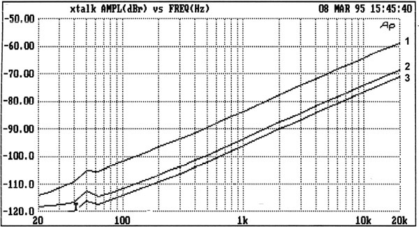
Crosstalk at low frequencies (below 1 kHz) was pleasingly low, being better than −129 dB up to 70 Hz, which was the difference between the noise floor and the maximum signal level. (The measured noise floor was unusually low at −114 dBu because each input amplifier was a quadruple noise cancelling type as described in Chapter 1, and that figure includes the noise from an AP System 1.) At higher frequencies things were rather less gratifying, being −96 dB at 10 kHz, as shown by the “47R” trace in Figure 2.3. In many applications this would be more than acceptable, but in this case the highest performance possible was being sought.

I therefore decided to reduce the output isolating resistors to 10 Ω so the interchannel capacitance would have less effect. (Checks were done at the time and all through the prototyping and preproduction process to make sure that this would be enough resistance to ensure opamp stability—it was.) This handily reduced the crosstalk to −109 dB at 10 kHz, an improvement of 13 dB at zero cost. This is the ratio between the two resistor values.

The third trace, marked “DIS”, shows the result of removing the isolating resistor from the speaking channel, so no signal reached the biamping switch. As usual, this reveals a further crosstalk mechanism, at about −117 dB, for reducing crosstalk is proverbially like peeling onions. There is layer after layer, and even strong men are reduced to tears.

Resistors

In the past there have been many types of resistor, including some interesting ones consisting of jars of liquid, but only a few kinds are likely to be met with now. (Jars of liquid are still used as resistances in high-voltage testing because of their ability to absorb huge amounts of peak power.) These are usually classified by the kind of material used in the resistive element, as this has the most important influence on the fine details of performance. The major materials and types are shown in Table 2.4.

These values are illustrative only, and it would be easy to find exceptions. As always, the official data sheet for the component you have chosen is the essential reference. The voltage coefficient is a measure of linearity (lower is better), and its sinister significance is explained later.

It should be said that you are most unlikely to come across carbon composition resistors in modern signal circuitry, but they frequently appear in vintage valve equipment so they are included here. They also live on in specialised applications such as switch-mode snubbing circuits, where their ability to absorb a high peak power in a mass of material rather than a thin film is very useful.

Carbon film resistors are currently still sometimes used in low-end consumer equipment, but elsewhere have been supplanted by the other three types. Note from Table 2.4 that they have a significant voltage coefficient.

Metal film resistors are now the usual choice when any degree of precision or stability is required. These have no nonlinearity problems at normal signal levels. The voltage coefficient is usually negligible.

Metal oxide resistors are more problematic. Cermet resistors and resistor packages are metal oxide and are made of the same material as thick film SM resistors. thick film resistors can show significant nonlinearity at opamp-type signal levels and should be kept out of high-quality signal paths.

Wirewound resistors are indispensable when serious power needs to be handled. The average wirewound resistor can withstand very large amounts of pulse power for short periods, but in this litigious age component manufacturers are often very reluctant to publish specifications on this capability, and endurance tests have to be done at the design stage; if this part of the system is built first then it will be tested as development proceeds. The voltage coefficient of wirewound resistors is usually negligible.

Table 2.4 Characteristics of resistor types

Type	Resistance tolerance	Temperature coefficient	Voltage coefficient
Carbon composition	±10%	+400 to −900 ppm/°	350 ppm
Carbon film	±5%	−100 to −700 ppm/°C	100 ppm
Metal film	±1%	+100 ppm/°C	1 ppm
Metal oxide	±5%	+300 ppm/°C	variable but too high
Wirewound	±5%	±70% to ±250%	1 ppm

Resistors for general PCB use come in both through-hole and surface-mount types. Through-hole (TH) resistors can be any of the types in Table 2.4; surface-mount (SM) resistors are always either metal film or metal oxide. There are also many specialised types; for example, high-power wirewound resistors are often constructed inside a metal case that can be bolted down to a heatsink.

Through-Hole Resistors

These are too familiar to require much description; they are available in all the materials mentioned earlier: carbon film, metal film, metal oxide, and wirewound. There are a few other sorts, such as metal foil, but they are restricted to specialised applications. Conventional through-hole resistors are now almost always 250 mW 1% metal film. Carbon film used to be the standard resistor material, with the expensive metal film resistors reserved for critical places in circuitry where low tempco and an absence of excess noise were really important, but as metal film got cheaper so it took over many applications.

TH resistors have the advantage that their power and voltage rating greatly exceed those of surface-mount versions. They also have a very low voltage coefficient, which for our purposes is of the first importance. On the downside, the spiral construction of the resistance element means they have much greater parasitic inductance; this is not a problem in audio work.

Surface-Mount Resistors

Surface-mount resistors come in two main formats, the common chip type and the rarer (and much more expensive) MELF format.

Chip surface-mount (SM) resistors come in a flat tombstone format, which varies over a wide size range; see Table 2.5.

MELF surface-mount resistors have a cylindrical body with metal endcaps, the resistive element is metal film, and the linearity is therefore as good as conventional resistors, with a voltage coefficient of less than 1 ppm. MELF is apparently an acronym for “Metal ELectrode Face-bonded”, though most people I know call them “Metal Ended Little Fellows” or something quite close to that.

Table 2.5 The standard surface-mount resistor sizes with typical ratings

Size L x W	Max power dissipation	Max voltage
2512	1 W	200 V
1812	750 mW	200 V
1206	250 mW	200 V
0805	125 mW	150 V
0603	100 mW	75 V
0402	100 mW	50 V
0201	50 mW	25 V
01005	30 mW	15 V

Surface-mount resistors may have thin film or thick film resistive elements. The latter are cheaper and so more often encountered, but the price differential has been falling in recent years. Both thin film and thick film SM resistors use laser trimming to make fine adjustments of resistance value during the manufacturing process. There are important differences in their behaviour.

Thin film (metal film) SM resistors use a nickel- chromium (Ni-Cr) film as the resistance material. A very thin Ni-Cr film of less than 1 um thickness is deposited on the aluminium oxide substrate by sputtering under vacuum. Ni-Cr is then applied onto the substrate as conducting electrodes. The use of a metal film as the resistance material allows thin film resistors to provide a very low temperature coefficient, much lower current noise and vanishingly small nonlinearity. Thin film resistors need only low laser power for trimming (one-third of that required for thick film resistors) and contain no glass-based material. This prevents possible micro-cracking during laser trimming and maintains the stability of the thin film resistor types.

Thick film resistors normally use ruthenium oxide (RuO₂) as the resistance material, mixed with glass-based material to form a paste for printing on the substrate. The thickness of the printing material is usually 12 um. The heat generated during laser trimming can cause micro-cracks on a thick film resistor containing glass-based materials which can adversely affect stability. Palladium/silver (PdAg) is used for the electrodes.

The most important thing about thick film surface-mount resistors from our point of view is that they do not obey Ohm’s law very well. This often comes as a shock to people who are used to TH resistors, which have been the highly linear metal film type for many years. They have much higher voltage coefficients than TH resistors, at between 30 and 100 ppm. The nonlinearity is symmetrical around zero voltage and so gives rise to third- harmonic distortion. Some SM resistor manufacturers do not specify voltage coefficient, which usually means it can vary disturbingly between different batches and different values of the same component, and this can have dire results on the repeatability of design performance.

Chip-type surface-mount resistors come in standard formats with names based on size, such as 1206, 0805, 0603 and 0402. For example, 0805, which used to be something like the “standard” size, is 0.08 in by 0.05 in; see Table 2.5. The smaller 0603 is now more common. Both 0805 and 0603 can be placed manually if you have a steady hand and a good magnifying glass.

The 0402 size is so small that the resistors look rather like grains of pepper; manual placing is not really feasible. They are only used in equipment where small size is critical, such as mobile phones. They have very restricted voltage and power ratings, typically 50V and 100 mW. The voltage rating of TH resistors can usually be ignored, as power dissipation is almost always the limiting factor, but with SM resistors it must be kept firmly in mind.

Recently, even smaller surface-mount resistors have been introduced; for example several vendors offer 0201, and Panasonic and Yageo offer 01005 resistors. The latter are truly tiny, being about 0.4 mm long; a thousand of them weigh less than a twentieth of a gram. They are intended for mobile phones, palmtops, and hearing aids; a full range of values is available from 10 Ω to 1 MΩ (jumper inclusive). Hand placing is really not an option.

Surface-mount resistors have a limited power-dissipation capability compared with their through-hole cousins, because of their small physical size. SM voltage ratings are also restricted, for the same reason. It is therefore sometimes necessary to use two SM resistors in series or parallel to meet these demands, as this is usually more economic than hand-fitting a through-hole component of adequate rating. If the voltage rating is the issue then the SM resistors will obviously have to be connected in series to gain any benefit.

Resistor Tolerances

As noted in Table 2.4, the most common tolerance for metal film resistors today is 1%; there is not likely to be much if any economic incentive to use 2% or even 5% parts. It is perhaps surprising that 5% carbon film resistors are still so freely available; a quick survey of distributors shows that they are not much cheaper than metal film. For some resistances in a phono amplifier 5% would be quite adequate; for example DC drain resistors or output isolation resistors. However in phono amplifiers most resistors need to be accurate, and it is unlikely to be worthwhile keeping two different resistor tolerances in stock, even if DC drain resistors are standardised at 22 kΩ and output isolation resistors at 47 Ω (which is quite feasible).

If you want a closer tolerance than 1%, then the next that is readily available in metal film is 0.1%; a few 0.5% resistor ranges are available, but they seem to be specialised parts with high power ratings and are not relevant to phono amplifiers. While there is considerable variation in the price of 0.1% resistors, roughly speaking they will be from 10 to 15 times more expensive than 1%. Very roughly, at the time of writing they are going to come in at something like 15p each, which I think is really quite reasonable considering their accuracy. Even so, it will usually be best to keep 0.1% for critical components; it helps if every critical resistance can be made the same nominal value, or at least there are only a few values, as this increases purchasing power and eases stock issues. For an example of this see The Devinyliser in Chapter 12, where only two different 0.1% values are used.

If 0.1% is not accurate enough—which I think it always will be for audio use—you can go to 0.05%, but then you are paying three or four GBP for each part. At about 10 GBP each, 0.02% can also be had, 0.01% at around 15 GBP each, and 0.005% at about 25 GBP. Clearly you are going to have to be working at the highest of the high end for this to make any vestige of economic sense. It might be marketing but it’s not engineering.

Resistor Selection for Awkward Values

Phono amplifiers are one of the notable fields of electronics where nonpreferred component values come up, due to the need for accurate RIAA equalisation. Awkward values are also likely to occur in subsonic and ultrasonic filters. The other big field for awkward values is active crossover design, where the crossover filters need to be accurate.

Resistors are widely available in the E24 series (twenty- four values per decade) and the E96 series (ninety-six values per decade). There is also the E192 series (you guessed it, 192 values per decade), but this is less freely available. The E3 and E6 series are used for capacitors. E3, E6, E12, E24 and E96 values are listed in Appendix 1. A quirk of this system is that while E3, E6, and E12 are all subsets of E24, and E96 is a subset of E192, E24 is not a subset of E96. Very few of the E24 values appear in E96. If you look for, say, the E24 value of 300 Ω in E96 you will not find it; the nearest values are 294 Ω and 301 Ω. There is an E48 series (every other value from E96), but it seems to get little or no use. I have never come across it in the wild. Appendix 1 also lists pairs of resistors in integer ratios for each series. For example, there are six E24 pairs in a 1:2 ratio, such as 120Ω–240Ω; these a very useful for building 2nd-order Butterworth highpass filters. Similarly, there are two E24 pairs in a 1:4 ratio (300Ω–1200Ω, 750Ω–3000Ω) which occurs in two-stage 3rd-order Butterworth highpass filters. See Chapter 12.

Using the E96 or, worse, the E192 series means that if, like me, you make many short production runs, to be able to get whatever value required you have to keep an enormous number of different resistor values in stock; when non-E24 values are required it is usually more convenient to use a series or parallel combination of two E24 resistors.

So, faced with what is effectively a random resistance value, what do you do? Here are three ways to address the problem. In Chapter 12 on subsonic filtering, thirty- six effectively random resistor values were dealt with in this way, and the averaged results for accuracy of the nominal value come from there.

1. 1) Use the nearest E96 value and keep your fingers crossed; this is simple, but the way that requires the least thought is rarely the best way. The accuracy will simply be that of the resistor series chosen. Despite the close spacing of the values, at about 2%, E96 resistors are often available at 1% tolerance.
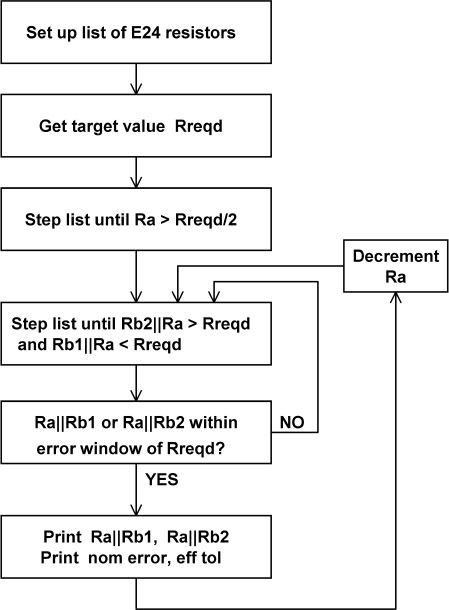
   I call this the 1xE96 format. The average absolute error for 1xE96 was 0.805%.
2. 2) Use two E24 1% resistors Ra, Rb in parallel, making them as equal as possible to get the best reduction in effective tolerance. I call this the 2xE24 format. It is often necessary to balance accuracy of nominal value against reduction of effective tolerance. I normally use the criterion that the nominal value should be accurate to better than half of the resistor tolerance; i.e. an error window of ±0.5%. Once that is achieved reduction in effective tolerance can be pursued. Writing some code that explores all the combinations of two resistors in parallel is straightforward; you set up a list of the E24 values, input the desired value Rreqd, then step through the list until you find the first resistor Ra that is greater than twice Rreqd. Put another resistor Rb from the E24 list in parallel; evaluate the combination, and keep at it until you have bracketed the required value with one result Rb1 too high and the other result Rb2 too low. If neither answer is within the error window, you know that an answer is impossible with that value of Ra. Increase Ra by one E24 step, then go round the loop again looking for bracketing values of Rb. When an answer is found within the error window, print the resistor values, the error in the nominal value, and the effective tolerance. However, do not stop; reduce Ra to the next lower E24 value and repeat. This will give you a series of bracketing values for Rb so you can choose the best solution. This process was used to generate all the 2xE24 resistor pairs in this book, and inevitably some have a more accurate nominal value than others. I have attempted to explain the algorithm in a good old-fashioned flowchart in Figure 2.4.
   The average absolute error in Chapter 12 for 2xE24 was 0.285%, which is three times better than 1xE96. The average effective tolerance, assuming 1% resistors, was 0.764%, which is not far from 0.707%, the best possible figure (this is explained in detail shortly).
3. 3) Using three E24 1% resistors in parallel not only allows us to get much closer to a desired nominal value, but also gives a better chance of getting near-equal resistors that give most of the potential 1/√3 (= 0.577) improvement in accuracy, because there are more combinations. The design process is not obvious; I used a Willmann table, which lists, in order of combined value, all combinations of three E24 resistors that give a combined value within a decade. The Willmann process is fully explained in Chapter 7 by means of practical examples in the design of RIAA equalisation networks. This book only makes use of the 3xE24 Willmann table; there are however many more that list E12, E48, and E96 combinations, etc. Gert Willmann intends to make the tables available as free software under the terms of the so-called GNU Lesser General Public License (LGPL); for more details, see www.gnu.org/licenses/. By the time this book is published the tables will be available free of charge either on my website or a site managed by Gert.
   The brute-force search used for 2xE24 does not look promising for dealing with three resistors because of the large number of combinations available.
   I call this the 3xE24 format. The average absolute error in Chapter 12 for 3xE24 was only 0.025%, more than ten times better than 2xE24. The average effective tolerance, assuming 1% resistors, was 0.659%, which is not too far from 0.577%, the best possible figure.
4. 4) This does not exhaust the possibilities. You could use four E24 resistors (4xE24) to get phenomenally accurate nominal values, but there is not much point unless the component tolerance is upgraded to 0.1% or better. Likewise you could use two E96 values (2xE96) or even three (3xE96) to get very accurate nominal values, but again the component tolerance will be the ultimate limit on the overall accuracy. Four or five paralleled capacitors are often very useful in RIAA networks–see Chapters 7 and 17.

Improving the Effective Tolerance

Using two, three, or more resistors to make up a desired value has a valuable hidden benefit. It will actually increase the average accuracy of the total resistance value, so it is better than the tolerance of the individual resistors; this may sound paradoxical, but it is simply an expression of the fact that random errors tend to partly cancel out if you have a number of them. This also works for capacitors, and indeed any parameter that is subject to random variations. Note that this assumes that the mean (i.e. average) value of the resistors is accurate. It is generally a sound assumption as it is much easier to control a single value such as the mean in a manufacturing process than to control all the variables that lead to scatter about that mean. This is confirmed by measurement.

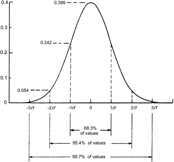
Component values are usually subject to a Gaussian distribution, also called a normal distribution. It has a familiar peaky shape, not unlike a resonance curve, showing that the majority of the values lie near the central mean and that they get rarer the further away from the mean you look. This is a very common distribution, cropping up wherever there are many independent things going on that affect the value of a given component. The distribution is defined by its mean and its standard deviation, which is the square root of the sum of the squares of the distances from the mean—the rms-sum, in other words. Sigma (σ) is the standard symbol for standard deviation. A Gaussian distribution will have 68.3% of its values within ±1 σ, 95.4% within ±2 σ, 99.7% within ±3 σ, and 99.9% within ±4 σ. This is illustrated in Figure 2.5, where the X-axis is calibrated in numbers of standard deviations on either side of the central mean value.

If we put two equal-value resistors in series, or in parallel (see Figure 2.6a and 2.6b), the total value has proportionally a narrower distribution that of the original components. The standard deviation of summed components is the rms-sum of the individual standard deviations, as shown in Equation 2.2; σ_sum is the overall standard deviation, and σ₁ and σ₂ are the standard deviations of the two resistors in series or parallel.

${\sigma }_{sum}=\sqrt{{\text{(}{\sigma }_1\text{)}}^2+{\text{(}{\sigma }_2\text{)}}^2}$

2.2

Equation 2.2 is only correct if there is no correlation between the two resistor values; this is true for two separate resistors but would not hold for two film resistors on the same substrate.

Thus if we have four 100 Ω 1% resistors in series, the standard deviation of the total resistance increases only by the square root of 4, that is two times, while the total resistance has increased by four times; thus we have made a 0.5% close-tolerance 400 Ω resistor for four times the price, whereas a 0.1% resistor would be at least ten and maybe fifteen times the price and may give more accuracy than we need. There is a happy analogue here with the use of multiple amplifiers to reduce electrical noise; we are using essentially the same technique of rms-summation to reduce “statistical noise”.

You may object that putting four 1% resistors in series means that the worst-case errors can be four times as great. This is obviously true—if they are all 1% low or 1% high, the total error will be 4%. But the probability of this occurring is actually very, very small indeed. The more resistors you combine, the more the values cluster together in the centre of the range.

The mathematics for series resistors is very simple; see Equation 2.2, which also holds for two parallel resistors as in Figure 2.6b, though this is mathematically much less obvious. Other resistor networks get complicated very quickly. I verified it by the use of Monte-Carlo methods.[4] A suitable random number generator is used to select two resistor values, and their combined value is calculated and recorded. This is repeated many times (by computer, obviously), and then the mean and standard deviation of all the accumulated numbers is recorded. This will never give the exact answer, but it will get closer and closer as you make more trials. For the series and parallel cases the standard deviation is 1/√2 of the standard deviation for a single resistor. If you are not wholly satisfied that this apparently magical improvement in average accuracy is genuine, seeing it happen on a spreadsheet makes a convincing demonstration.

In an Excel spreadsheet, random numbers with a uniform distribution are generated by the function RAND(), but random numbers with a Gaussian distribution and specified mean and standard deviation can be generated by the function NORMINV(). Let us assume we want to make an accurate 20 kΩ resistance. We can simulate the use of a single 1% tolerance resistor by generating a column of Gaussian random numbers with a mean of 20 and a standard deviation of 0.2; we need to use a lot of numbers to smooth out the statistical fluctuations, so we generate 400 of them. As a check we calculate the mean and standard deviation of our 400 random numbers using the AVERAGE() and STDEV() functions. The results will be very close to 20 and 0.2, but not identical, and will change every time we hit the F9 recalculate key because this generates a new set of random numbers. The results of five recalculations are shown in Table 2.6, demonstrating that 400 numbers are enough to get us quite close to our targets.

To simulate two 10 kΩ resistors of 1% tolerance in series we generate two columns of 400 Gaussian random numbers with a mean of 10 and a standard deviation of 0.1. We then set up a third column which is the sum of the two random numbers on the same row, and if we calculate the mean and standard deviation using AVERAGE() and STDEV() again, we find that the mean is still very close to 20 but the standard deviation is reduced on average by the expected factor of √2. The result of five trials is shown in Table 2.7. Repeating this experiment with two 40 kΩ resistors in parallel gives the same results.

If we repeat this experiment by making our 20 kΩ resistance from a series combination of four 5 kΩ resistors of 1% tolerance we generate four columns of 400 Gaussian random numbers with a mean of 5 and a standard deviation of 0.05. We sum the four numbers on the same row to get a fifth column and calculate the mean and standard deviation of that. The result of five trials is shown in Table 2.8. The mean is very close to 20, but the standard deviation is now reduced on average by a factor of √4, which is 2.

I think this demonstrates quite convincingly that the spread of values is reduced by a factor equal to the square root of the number of the components used. The principle works equally well for capacitors or indeed any quantity with a Gaussian distribution of values. The downside is the fact that the improvement depends on the square root of the number of equal-value components used, which means that big improvements require a lot of parts and the method quickly gets unwieldy. Table 2.9 demonstrates how this works; the rate of improvement slows down noticeably as the number of parts increases. The largest number of components I have ever used in this way for a production design is five; see Chapter 17.

Table 2.6 Mean and standard deviation of five batches of 400 Gaussian random resistor values

Mean kΩ	Standard deviation
20.0017	0.2125
19.9950	0.2083
19.9910	0.1971
19.9955	0.2084
20.0204	0.2040

Table 2.7 Mean and standard deviation of five batches of 400 Gaussian 10 kΩ 1% resistors, two in series

Mean kΩ	Standard deviation
19.9999	0.1434
20.0007	0.1297
19.9963	0.1350
20.0114	0.1439
20.0052	0.1332

Table 2.8 Mean and standard deviation of five batches of 400 Gaussian 5 kΩ 1% resistors, four in series

Mean kΩ	Standard deviation
20.0008	0.1005
19.9956	0.0995
19.9917	0.1015
20.0032	0.1037
20.0020	0.0930

But what happens if the series resistors used are not equal? The overall standard deviation is still the rms-sum of the standard deviations of the two resistors, as shown in Equation 2.2. Since both resistors have the same percentage tolerance, the larger of the two has the greater standard deviation and dominates the total result. The minimum total deviation is thus achieved with equal resistor values.

Table 2.9 The improvement in value tolerance with number of equal-value parts

Number of equal-value parts	Tolerance reduction factor
1	1.000
2	0.707
3	0.577
4	0.500
5	0.447
6	0.408
7	0.378
8	0.354
9	0.333
10	0.316

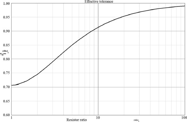
Figure 2.7 shows how this works for either series or parallel connection. As the resistors move away from a ratio of 1:1 the effective tolerance quickly degrades from 0.707%, but using two resistors in the ratio 2:1 or 3:1 still gives a worthwhile improvement. Much larger ratios, which may be required to get a given nominal value, still show some improvement, but it slowly falls off and asymptotes to 1.0, where one resistor of the pair effectively does not exist at all. The plot is based on a 1% resistor tolerance, but any other tolerance behaves proportionally.

Other Resistor Networks

So far we have looked at serial and parallel combinations of components to make up one value, as in Figure 2.6a, b. Other important networks are the resistive divider in Figure 2.6c, (frequently used as the negative- feedback network for noninverting amplifiers) and the inverting amplifier in Figure 2.6f, where the gain is set by the ratio R2/R1. All resistors are assumed to have the same tolerance about an exact mean value.

I suggest it is not obvious whether the divider ratio of Figure 2.6c, which is R2/(R1 + R2), will be more or less accurate than the resistor tolerance. In the simplest case with R1 = R2 the Monte-Carlo method shows that partial cancellation of errors still occurs and the division ratio is improved in accuracy by a factor of √2.

However—this factor actually depends on the divider ratio, as a simple physical argument shows:

• If the top resistor R1 is zero, then the divider ratio is obviously one with complete accuracy, the resistor values are irrelevant, and the output voltage tolerance is zero.
• If the bottom resistor R2 is zero, there is no output and accuracy is meaningless, but if instead R2 is very small compared with R1 then the R1 completely determines the current through R2, and R2 turns this into the output voltage. Therefore the tolerances of R1 and R2 act independently, and so the combined output voltage tolerance is worse by their rms-sum, which is √2.

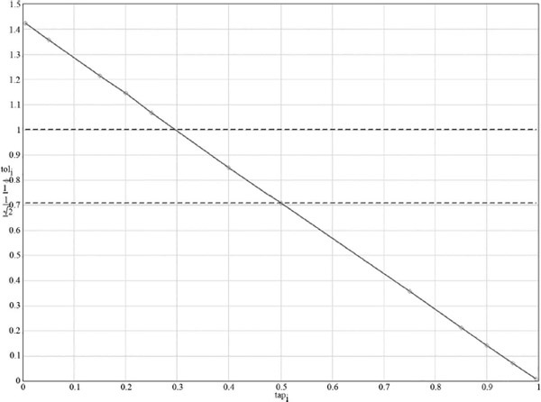
Some more Monte-Carlo work, with 8000 trials per data point, revealed that there is a linear relationship between accuracy and the “tap position” of the output between R1 and R2, as shown in Figure 2.8. Plotting against division ratio would not give a straight line. With R1 = R2 the tap is at 50% and accuracy improved by a factor of √2, as noted earlier. With a tap at about 30% (R1 = 7 kΩ, R2 = 3 kΩ) the accuracy is the same as the resistors used. This assessment is not applicable to potentiometers as the two sections of the pot are not uncorrelated; in linear pots they are very much correlated.

The two-tap divider (Figure 2.6d) and three-tap divider (Figure 2.6e) were also tested with equal resistors. The two-tap divider has an accuracy factor of 0.404 at OUT 1 and 0.809 at OUT 2. These numbers are very close to √2/(2√3) and √2/(√3) respectively. The three-tap divider has an accuracy factor of 0.289 at OUT 1, of 0.500 at OUT 2, and of 0.864 at OUT 3. The middle figure is clearly 1/2 (twice as many resistors as a one-tap divider, so √2 times more accurate), while the first and last numbers are very close to √3/6 and √3/2 respectively. It would be helpful if someone could prove analytically that the factors proposed are actually correct.

For the inverting amplifier of Figure 2.6f, the accuracy of the gain is always √2 worse than the tolerance of the two resistors, assuming the tolerances are equal. The nominal resistor values have no effect on this. We therefore have the interesting situation that a noninverting amplifier will always be equally or more accurate in its gain than an inverting amplifier. So far as I know this is a new result.

Resistor Pair Choice

In many cases the resistance value required is completely determined, and the only decision is how to make up the value with a pair that will meet the requirements for an accurate nominal value and for effective tolerance. However, sometimes there is an extra degree of freedom that allows more optimisation; this is an important point, and I am going to look at it in detail.

Consider the simple potential divider in Figure 2.6c, and we will assume we want exactly 3 dB of attenuation, which is 0.70795 times. The divider will be driven by an opamp, so we want to keep the loading reasonably light for good distortion performance; this implies the resistance to ground through the divider is not less than 1 kΩ. This suggests high resistor values should be used. The divider is feeding an opamp input, so we want a low value of divider output impedance to keep down Johnson noise and the effects of opamp input-current noise. This suggests low resistor values should be used, and a compromise is required. One more assumption—the top resistor R1 will be a single E24 part. To get an accurate 3dB of attenuation, R2 will therefore have to be a 2xE24 pair. Table 2.10 shows what happens when we pick various E24 values for R1 and then choose a parallel pair R2a, R2b with the criterion that the combined nominal value shall not be in error by more than 0.5% (1% resistors with an accurate mean value are assumed).

Loading and output impedance are calculated from the R2 column. Table 2.10 was arbitrarily started with a value of 1.5 kΩ for R1, which gives an output impedance of approximately 1 kΩ. The last value of 270 Ω for R1 brings the total resistance of the potential divider below 1 kΩ and so breaks our rules.

This shows using E24 resistors, accepting a minimal load resistance of 1 kΩ loading and a maximum output impedance of 1 kΩ, gives us no fewer than seventeen possible solutions for our potential divider. (If R1 was also made up of a 2xE24 pair, there would be a great many more) Which one we select depends on the circuit design priorities. If an accurate nominal value is the overriding concern, then R1 = 330 Ω gives a nominal error of only +0.004%, combined with an effective tolerance of 0.707 %, which is as good as it gets because the two resistors making up R2 are equal. The output impedance is nicely low at 234 Ω, which will have a Johnson noise of only −128.5 dBu (usual conditions). This looks the best solution out of the seventeen. The loading of the divider is relatively heavy at 1130 Ω, and if on second thoughts we would prefer a higher resistance, R1 = 680 Ω looks promising, with a nominal error of only +0.062 % and once more an effective tolerance of 0.707%. Other factors may come into play—if you have a huge stock of 620 Ω resistors, then R1 = 620 Ω looks more attractive.

Many other circumstances arise in circuit design, where there is a degree of freedom in choosing one component that allows the best option for another component to be selected.

Resistor Value Distributions

At this point you may be complaining that this will only work if the resistor values have a Gaussian (also known as normal) distribution with the familiar peak around the mean (average) value. Actually, it is a happy fact this effect does not assume that the component values have a Gaussian distribution; even a batch of resistors with a uniform distribution gives better accuracy when two of them are combined. This is easily demonstrated by Monte-Carlo. An excellent account of how to handle statistical variations to enhance accuracy is in W. J. Smith’s Modern Optical Engineering.[5] This deals with the addition of mechanical tolerances in optical instruments, but the principles are just the same.

You sometimes hear that this sort of thing is inherently flawed, because, for example, 1% resistors are selected from production runs of 5% resistors. If you were using the 5% resistors, then you would find there was a hole in the middle of the distribution; if you were trying to select 1% resistors from them, you would be in for a very frustrating time as they have already been selected out, and you wouldn’t find a single one. If instead you were using the 1% components obtained by selection from the complete 5% population, you would find that the distribution would be much flatter than Gaussian and the accuracy improvement obtained by combining them would be reduced, although there would still be a definite improvement.

However, don’t worry. In general this is not the way that components are manufactured nowadays, though it may have been so in the past. A rare contemporary exception is the manufacture of carbon composition resistors,[6] where making accurate values is difficult and selection from production runs, typically with a 10% tolerance, is the only practical way to get more accurate values. Carbon composition resistors have no place in audio circuitry because of their large temperature and voltage coefficients and high excess noise, but they live on in specialised applications such as switch-mode snubbing circuits, where their ability to absorb high peak power in bulk material rather than a thin film is useful, and in RF circuitry, where the inductance of spiral-format film resistors is unacceptable.

So, having laid that fear to rest, what is the actual distribution of resistor values like? It is not easy to find out, as manufacturers are not exactly forthcoming with this sort of sensitive information, and measuring thousands of resistors with an accurate DVM is not a pastime that appeals to all of us. Any nugget of information in this area is therefore very welcome.

Hugo Kroeze[7] reported the result of measuring 211 metal film resistors from the same batch with a nominal value of 10 kΩ and 1% tolerance. He concluded that:

1. 1) The mean value was 9.995 k Ω (0.05% low).
2. 2) The standard deviation was about 10 Ω, i.e. only 0.1%. This spread in value is surprisingly small (the resistors were all from the same batch, and the spread across batches widely separated in manufacture date might have been less impressive).
3. 3) All resistors were within the 1% tolerance range.
4. 4) The distribution appeared to be Gaussian, with no evidence that it was a subset from a larger distribution.

I decided to add my own morsel of data to this. I measured 100 ordinary metal film 1kΩ resistors of 1% tolerance from Yageo, a Chinese manufacturer, and very tedious it was too. I used a recently calibrated 4.5 digit meter.

1. 1) The mean value was 997.66 ohms (0.23% low).
2. 2) The standard deviation was 2.10 ohms, i.e. 0.21%.
3. 3) All resistors were within the 1% tolerance range. All but one was within 0.5%, with the outlier at 0.7%.
4. 4) The distribution appeared to be Gaussian, with no evidence that it was a subset from a larger distribution.

These are only two reports, but from this and other evidence there seems to be no reason to doubt that the mean value is very well controlled, and the spread is under good control as well. The distribution of resistance values appears to be Gaussian, with nothing selected out.

The Uniform Distribution

As I mentioned earlier, improving average accuracy by combining resistors does not depend on the resistance value having a Gaussian distribution. A uniform distribution of component values would seem to be very unlikely, but the result of combining two or more of them is highly instructive; two combined give a triangular-shaped distribution, combining more gives a shape that gets peakier and eventually is indistinguishable from the Gaussian distribution.

Resistor Imperfections

Ohm’s law strictly is a statement about metallic conductors only. It is dangerous to assume that it also invariably applies to “resistors” simply because they have a fixed value of resistance marked on them; in fact resistors—whose main raison d’etre is packing a lot of controlled resistance in a small space—do not always adhere to Ohm’s law very closely. This is a distinct difficulty when trying to make low-distortion circuitry.

It is well known that resistors have inductance and capacitance and vary somewhat in resistance with temperature. Unfortunately there are other less obvious imperfections, such as excess noise and nonlinearity; these can get forgotten because parameters describing how bad they are often omitted from component manufacturer’s data sheets.

Being components in the real world, resistors are not perfect examples of resistance and nothing else. Their length is not infinitely small, and so they have series inductance; this is particularly true for the many kinds that use a spiral resistive element. Likewise, they exhibit stray capacitance between each end and also between the various parts of the resistive element. Both effects can be significant at high frequencies, but can usually be ignored below 100 kHz unless you are using very high or low resistance values.

It is a sad fact that resistors change their value with temperature. Table 2.4 shows some typical temperature coefficients. This is not likely to be a problem in small-signal audio applications, where the ambient temperature range is usually small, and extreme precision is not required unless you are designing measurement equipment. Carbon film resistors are markedly inferior to metal film in this area.

The fact that resistors have non-zero temperature coefficients has however a worrying implication; if significant cyclic changes in temperature occur due to big low-frequency signals, there will be corresponding cyclic changes in resistance that in some circuit positions will cause nonlinear distortion. This is dealt with in more detail later, but in short it is unlikely to reach measurable proportions in metal film resistors unless the signal is bigger than 25 Vrms and the frequency below 100 Hz.

Many resistors also change their value slightly with the voltage placed across them; this is measured by the voltage coefficient and can cause frequency-insensitive nonlinear distortion. This is also dealt with in more detail later.

Resistor Excess Noise

All resistors, no matter what their resistive material or mode of construction, generate Johnson noise. This is white noise, its level being determined solely by the resistance value, the absolute temperature, and the bandwidth over which the noise is being measured. It is based on fundamental physics and is not subject to negotiation. Some cases it places the limit on how quiet a circuit can be, though the noise from active devices is often more significant. Johnson noise is covered in Chapter 1.

Excess resistor noise refers to the fact that some kinds of resistor, with a constant voltage drop imposed across them, generate excess noise in addition to its inherent Johnson noise. According to classical physics, passing a current through a resistor should have no effect on its noise behaviour; it should generate the same Johnson noise as a resistor with no steady current flow. In reality, some types of resistors do generate excess noise when they have a DC voltage across them. It is a very variable quantity, but is essentially proportional to the DC voltage across the component, a typical spec being “1 uV/V” and it has a 1/f frequency distribution. Typically it could be a problem in biasing networks at the input of amplifier stages. It is usually only of interest if you are using carbon or thick film resistors- metal film, and wirewound types should have very little excess noise. It is known 1/f noise does not have a Gaussian amplitude distribution, which makes it difficult to assess reliably from a small set of data points. A rough guide to the likely specs is given in Table 2.11.

(Wirewound resistors are normally considered to be completely free of excess noise.)

The level of excess resistor noise changes with resistor type, size, and value in ohms; here are the relevant factors:

Table 2.11 Resistor excess noise

Type	Noise uV/V
Metal film TH	0
Carbon film TH	0.2–3
Metal oxide TH	0.1–1
Thin film SM	0.05–0.4
Bulk metal foil TH	0.01
Wirewound TH	0

A physically large resistor has lower excess noise than a small resistor, because there is more resistive material in parallel, so to speak. In the same resistor range, the highest wattage versions have the lowest noise. See Figure 2.9.

A low ohmic value resistor has lower excess noise than a high ohmic value. Noise in uV per V rises approximately with the square root of resistance. See Figure 2.9 again.

A low value of excess noise is associated with uniform constriction-free current flow; this condition is not well met in composite thick film materials. However, there are great variations among different thick film resistors. The most readily apparent relationship is between noise level and the amount of conductive material present. Everything else being equal, compositions with lower resistivity have lower noise levels.

Higher resistance values give higher excess noise since it is a statistical phenomenon related to the total number of charge carriers available within the resistive element; the fewer the total number of carriers present, the greater will be the statistical fluctuation.

Traditionally at this point in the discussion of excess resistor noise, the reader is warned against using carbon composition resistors because of their very bad excess noise characteristics. Carbon composition resistors are still made—their construction makes them good at handling pulse loads—but are not likely to be encountered in audio circuitry.

One of the great benefits of dual-rail opamp circuitry is that is noticeably free of resistors with large DC voltages across them. The offset voltages and bias currents are far too low to cause trouble with resistor excess noise. However, if you are getting into low-noise hybrid discrete/opamp stages, such as the MC head amplifier in Chapter 12, you might have to consider it.

To get a feel for the magnitude of excess resistor noise, consider a 100 kΩ 1/4 W carbon film resistor with 10V across it. This, from the graph above, has an excess noise parameter of about 0.7 uV/V and so the excess noise will be of the order of 7 uV, which is −101 dBu. This definitely could be a problem in a low-noise preamplifier stage.

Resistor Nonlinearity: Voltage Coefficient

This form of resistor nonlinearity is normally quoted by manufacturers as a voltage coefficient, usually the number of parts per million (ppm) that the resistor value changes when one volt is applied. The measurement standard for resistor nonlinearity is IEC 6040.

Through-hole metal film resistors usually show perfect linearity at the levels of performance considered here, as do wirewound types. The voltage coefficient is less than 1 ppm. Carbon film resistors are quoted at less than 100 ppm; 100 ppm is however enough to completely dominate the distortion produced by active devices, if it is used in a critical part of the circuitry. Carbon composition resistors, probably of historical interest only, come in at about 350 ppm, a point that might be pondered by connoisseurs of antique equipment. The greatest area of concern over nonlinearity is thick film surface-mount resistors, which have high and rather variable voltage coefficients; more on this later.

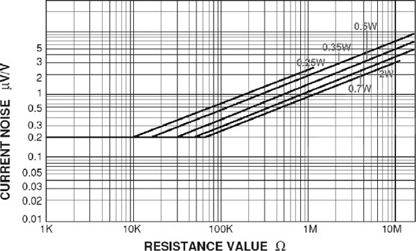
Table 2.12 (calculated with SPICE) gives the THD in the current flowing through the resistor for various voltage coefficients when a pure sine voltage is applied. If the voltage coefficient is significant this can be a serious source of nonlinearity.

Table 2.12 Resistor voltage coefficients and the resulting distortion at +15 and +20 dBu.

Voltage	THD at	THD at
Coefficient	+15 dBu	+20 dBu
1 ppm	0.00011 %	0.00019 %
3 ppm	0.00032 %	0.00056%
10 ppm	0.0016 %	0.0019 %
30 ppm	0.0032 %	0.0056 %
100 ppm	0.011 %	0.019 %
320 ppm	0.034 %	0.060 %
1000 ppm	0.11 %	0.19 %
3000 ppm	0.32 %	0.58 %

A voltage coefficient model generates all the odd-order harmonics, at a decreasing level as order increases. No even-order harmonics can occur because the model is symmetrical. This is covered in much more detail in my power amplifier book.[8]

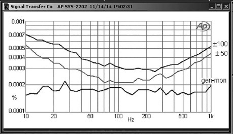
My own test setup is shown in Figure 2.10. The resistors are usually of equal value, to give 6 dB attenuation. A very low-distortion oscillator that can give a large output voltage is necessary; the results in Figure 2.11 were taken at a 10 Vrms (+22 dBu) input level. Here thick film SM and through-hole resistors are compared. The gen-mon trace at the bottom is the record of the analyser reading the oscillator output and is the measurement floor of the AP System 1 used. The TH plot is higher than this floor, but this is not due to distortion. It simply reflects the extra Johnson noise generated by two 10 kΩ resistors. Their parallel combination is 5 kΩ, and so this noise is at −115.2 dBu. The SM plot, however, is higher again, and the difference is the distortion generated by the thick film component.

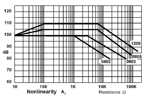
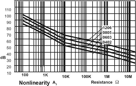
For both thin film and thick film SM resistors nonlinearity increases with resistor value and also increases as the physical size (and hence power rating) of the resistor shrinks. The thin film versions are much more linear; see Figures 2.12 and 2.13. Sometimes it is appropriate to reduce the nonlinearity by using multiple resistors in series. If one resistor is replaced by two with the same voltage coefficient in series, the THD in the current flowing is halved. Similarly, using three resistors reduces THD to a third of the original value. There are obvious economic limits to this sort of thing, but it can be useful in specific cases, especially where the voltage rating of the resistor is a limitation.

Modelling voltage coefficient distortion in SPICE simulation is straightforward. An analogue behavioural model is used to create a resistance whose value varies proportionally with the instantaneous voltage across it; a 1st-order voltage coefficient nonlinearity. Only odd harmonics are generated, and their percentage increases proportionally with the signal level. It is not much more complex to model a resistance whose value varies proportionally with the square of the instantaneous voltage; a 2nd-order voltage coefficient nonlinearity. Once more only odd harmonics appear, but in this case the third harmonic increases as the square of signal level, the fifth as the fourth power, and so on. The SPICE modelling of voltage coefficient nonlinearity is dealt with in much more detail in my book Audio Power Amplifier Design,[8] but make sure you get the 6th edition or later.

Resistor Nonlinearity: Temperature Coefficient

Since resistors have nonzero temperature coefficients it is obvious that if cyclic changes in temperature occur, there will be corresponding cyclic changes in resistance. If the resistor concerned is involved in setting the gain of the stage (for example as part of a voltage divider providing negative feedback), the cyclic changes in gain will cause nonlinear distortion. This is often called thermal distortion; there is much talk in the hi-fi world of “thermal distortion” in circumstances where it does not exist, but this example is the real thing. The lower the frequency, the greater the distortion, as the resistor has more time to change temperature. The distortion level rises very slowly as frequency falls, taking three octaves to double in amplitude, and as far as I am aware this behaviour is unique to thermal distortion and provides a good test for its existence. The distortion is reasonably pure third harmonic.

Thermal distortion in carbon film resistors is relatively easy to detect and measure; in a simple 6 dB voltage divider where only one part is carbon film, the other being metal film, it will be around 0.001% at 10 Hz and 20 Vrms. You can argue a) that’s not a lot of distortion, and b) 20 Vrms is not going to be encountered in small-signal design, except in a balanced output stage running at maximum level. The counterargument is that many resistors in a practical system, all showing that sort of distortion, are likely to give a rather unhappy overall result.

Generally, in small-signal design you can just specify metal film resistors and forget about the issue; an exception being a balanced line output at maximum level. It is a very real issue in power amplifiers of more than modest output, and this is a good way to demonstrate the effect with amounts of distortion that are easily measured. The feedback network will be a voltage divider with the upper resistor having almost all the output voltage across it; at 100W/8Ω this will be about 27 Vrms, and at this level even a high-quality metal film resistor has been found to generate 0.0008% THD+N at 10 Hz. You obviously need to use a really good and clean power amplifier, or other distortion mechanisms will mask the effect. I used one of my Blameless power amplifiers. Figure 2.14 shows the results at 100W/8Ω, where thermal distortion causes the gentle rise in THD +N below 100 Hz. The original feedback resistor had a temperature coefficient specified as 100 ppm/°C, and replacing it with a different type (from the same reputable manufacturer) spec’d at 50 ppm/°C gave significantly reduced distortion.

If you do run into thermal distortion, you might fear that a nonlinearity built into a passive component is going to be hard to cure. Not so. First the distortion is low, and reducing it by a factor of three or four times will usually push it below the noise floor. In dealing with voltage coefficient distortion we can split the signal voltage across two or more resistors in series. For thermal distortion we need to split the power, and either parallel or series connections can be used.

It is quite easy to model voltage coefficient distortion in SPICE simulation, but temperature coefficient distortion is a harder nut to crack. It is straightforward to calculate the instantaneous heat dissipation and combine that with the effective thermal inertia to calculate the cyclic resistance change. The problem is, the thermal inertia of what? It is the temperature of actual resistive element—the helical metal film—that matters, but it is intimately attached to the body of the resistor, which much affects the thermal inertia. The thermal variations inside the body will depend on the distance from the surface, and modelling the effects of this is probably going to require some sort of network of RC time-constants.

Capacitors

Capacitors are diverse components. In the audio business their capacitance ranges from 10 pF to 100,000 uF, a ratio of 10 to the tenth power. In this they handily out-do resistors, which usually vary from 0.1 Ω to 10 MΩ, a ratio of only 10 to the eighth. However, if you include the 10 GΩ bias resistors used in capacitor microphone head amplifiers, this range increases to 10 to the eleventh. There is however a big gap between the 10 MΩ resistors, which are used in DC servos and 10 GΩ microphone resistors; I am not aware of any audio applications for 1 GΩ resistors.

Capacitors also come in a wide variety of types of dielectric, the great divide being between electrolytic and nonelectrolytic types. Electrolytics used to have much wider tolerances than most components, but things have recently improved, and ±20% is now common. This is still wider than for typical nonelectrolytics, which are usually ±10% or better.

This is not the place to reiterate the basic information about capacitor properties, which can be found from many sources. I will simply note that real capacitors fall short of the ideal circuit element in several ways, notably leakage, equivalent series resistance (ESR), dielectric absorption and nonlinearity: Capacitor leakage is equivalent to a high-value resistance across the capacitor terminals and allows a trickle of current to flow when a DC voltage is applied. It is usually negligible for nonelectrolytics, but is much greater for electrolytics.

ESR is a measure of how much the component deviates from a mathematically pure capacitance. The series resistance is partly due to the physical resistance of leads and foils and partly due to losses in the dielectric. It can also be expressed as tan-δ (tan-delta). Tan-delta is the tangent of the phase angle between the voltage across and the current flowing through the capacitor.

Dielectric absorption is a well-known phenomenon; take a large electrolytic, charge it up, and then make sure it is fully discharged. Use a 10 Ω WW resistor across the terminals rather than a screwdriver unless you’re not too worried about either the screwdriver or the capacitor. Wait a few minutes, and the charge will partially reappear, as if from nowhere. This “memory effect” also occurs in nonelectrolytics to a lesser degree; it is a property of the dielectric and is minimised by using polystyrene, polypropylene, NPO ceramic, or PTFE dielectrics. Dielectric absorption is invariably simulated by a linear model composed of extra resistors and capacitances; nevertheless, dielectric absorption and distortion correlate across the different dielectrics.

Capacitor nonlinearity is undoubtedly the least known of these shortcomings. A typical RC lowpass filter can be made with a series resistor and a shunt capacitor, and if you examine the output with a distortion analyser, you may find to your consternation that the circuit is not linear. If the capacitor is a nonelectrolytic type with a dielectric such as polyester, then the distortion is relatively pure third harmonic, showing that the effect is symmetrical. For a 10 Vrms input, the THD level may be 0.001% or more. This may not sound like much, but it is substantially greater than the mid-band distortion of a good opamp. Capacitor nonlinearity is dealt with at greater length later.

Capacitors are used in audio circuitry for three main functions, where their possible nonlinearity has varying consequences:

1. 1) Coupling or DC-blocking capacitors. These are usually electrolytics, and if properly sized have a negligible signal voltage across them at the lowest frequencies of interest. Likewise, the detailed properties of the capacitor are unimportant unless they have power amplifier current levels through them; power amplifier output capacitors can generate considerable mid-band distortion.[9] Much nonsense has been talked about mysterious coupling capacitor properties, but it is all absolute and total nonsense. For small-signal use, as long as the signal voltage across the capacitor is kept low, nonlinearity is not normally detectable. The capacitance value must be noncritical, given the wide tolerances of electrolytics.
2. 2) Supply filtering or decoupling capacitors. These are electrolytics if you are filtering out supply rail ripple, etc., and non-electrolytics, usually around 100 nF, when the task is to keep the supply impedance low at high frequencies and so keep opamps stable. The capacitance value is again noncritical.
3. 3) Setting time-constants, for example the capacitors in the feedback network of an RIAA amplifier. This is a much more demanding application than the other two. First, the actual value is now crucially important as it defines the accuracy of the frequency response. Second, there is by definition significant signal voltage across the capacitor, as it is involved in filtering, and so nonlinearity can be a serious problem. Nonelectrolytics are normally used; sometimes an electrolytic is used to define the lower end of the bandwidth, but this is a bad practice likely to introduce distortion at the bottom of the frequency range. Small value ceramic capacitors are used for compensation purposes.

In Subjectivist circles it is frequently asserted that electrolytic coupling capacitors (if they are permitted at all) should be bypassed by small nonelectrolytics. There is no sense in this; if the main coupling capacitor has no signal voltage across it, the extra capacitor can have no effect.

Capacitor Selection for Awkward Values

There is much discussion in this book about the best way to obtain awkward resistance values; this is relatively easy because resistors are available in the E24 series. Capacitors are different; they are frequently only obtainable in the E3, E6, or E12 series. This makes the mathematical problem quite different—one approach is to select the nearest capacitor that is smaller than the desired value, then parallel smaller and smaller capacitors until you get as close as desired. A better way is to try to break the capacitance into two or three equal values, plus an extra capacitor, as this gives more improvement in the effective tolerance.

Another factor is the need for a close tolerance on the capacitor value. As explained in more detail in Chapter 7, often the most economical way to get a 1% tolerance is to use polystyrene capacitors, but in many ranges 10 nF is the largest available value, and for phono amplifier use several may need to be paralleled. This improves the effective tolerance in the same way as for resistors. There are many examples of this in Chapter 7. Most of the capacitor combinations in this book were produced manually, but since then Gert Willmann has produced a table for four E6 capacitors in parallel. It is 3360 lines long, but this is perfectly easy to handle and search in any decent text editor.

I used this new table to check all the values for C2 in Chapter 7, where three or four capacitors are used in parallel, and was rather surprised that only two out of ten results could be improved. These are shown in Tables 2.13 and 2.14. In the first table the use of four capacitors rather than three allows the nominal error to be reduced from +0.28% to a negligible 0.01%, with a helpful improvement in the effective tolerance.

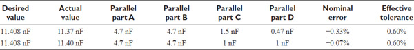
In Table 2.14 four capacitors are used in each case

These new values have been used in Chapter 7.

Capacitor Nonlinearity Examined

When attempting the design of linear circuitry, everyone knows that inductors and transformers with ferromagnetic core material can be a source of nonlinearity. It is however less obvious that capacitors and even resistors can show nonlinearity and generate some unexpected and very unwelcome distortion. Resistor nonlinearity has been dealt with earlier in this chapter; let us examine the shortcomings of capacitors.

The definitive work on capacitor distortion is a magnificent series of articles by Cyril Bateman in Electronics World.[10] The authority of this work is underpinned by Cyril’s background in capacitor manufacture. (The series is long because it includes the development of a low-distortion THD test set in the first two parts.)

Capacitors generate distortion when they are actually implementing a time-constant—in other words, when there is a signal voltage across them. The normal coupling or DC-blocking capacitors have no significant signal voltage across them, as they are intended to pass all the information through, not to filter it or define the system bandwidth. Capacitors with no signal across them do not generally produce distortion at small-signal current levels. This was confirmed for all the capacitors tested here. However, electrolytic types may do so at power amplifier levels where the current through them is considerable, such as in the output coupling capacitor of a power amplifier.[9]

Nonelectrolytic Capacitor Nonlinearity

It has often been assumed that nonelectrolytic capacitors, which generally approach an ideal component more closely than electrolytics and have dielectrics constructed in a totally different way, are free from distortion. It is not so. Some nonelectrolytics show distortion at levels that are easily measured and can exceed the distortion from the opamps in the circuit. Nonelectrolytic capacitor distortion is primarily third harmonic, because the nonpolarised dielectric technology is basically symmetrical. The problem is serious, because nonelectrolytic capacitors are commonly used to define time-constants and frequency responses (in RIAA equalisation networks, for example) rather than simply for DC blocking.

Very small capacitances present no great problem. Simply make sure you are using the COG (NP0) type, and so long as you choose a reputable supplier, there will be no distortion. I say “reputable supplier” because I did once encounter some allegedly COG capacitors from China that showed significant nonlinearity.[11]

Middle-range capacitors, from 1 nF to 1 uF, present more of a problem. Capacitors with a variety of dielectrics are available, including polyester, polystyrene, polypropylene, polycarbonate, and polyphenylene sulphide, of which the first three are the most common. (Note that what is commonly called “polyester” is actually polyethylene terephthalate, PET.)

Figure 2.15 shows a simple lowpass filter circuit which, in conjunction with a good THD analyser, can be used to get some insight into the distortion problem; it is intended to be representative of a real bit of audio circuitry. The values shown give a pole frequency, or −3 dB roll-off point, at 710 Hz. Since it might be expected that different dielectrics give different results (and they definitely do), we will start off with polyester, the smallest, most economical, and therefore the most common type for capacitors of this size.

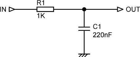
The THD results for a microbox 220 nF 100 V capacitor with a polyester dielectric are shown in Figure 2.16, for input voltages of 10, 15, and 20 Vrms. They are unsettling.

The distortion is all third harmonic and peaks at around 300 to 400 Hz, well below the pole frequency, and even with input limited to 10 Vrms, will exceed the nonlinearity introduced by opamps such as the 5532 and the LM4562. Interestingly, the peak frequency changes with applied level. Below the peak, the voltage across the capacitor is constant, but distortion falls as frequency is reduced, because the increasing impedance of the capacitor means it has less effect on a circuit node at a 1 kΩ impedance. Above the peak, distortion falls with increasing frequency because the lowpass circuit action causes the voltage across the capacitor to fall.

The level of distortion varies with different samples of the same type of capacitor; six of this type were measured, and the THD at 10 Vrms and 400 Hz varied from 0.00128% to 0.00206%. This puts paid to any plans for reducing the distortion by some sort of cancellation method. The distortion can be seen in Figure 2.16 to be a strong function of level, roughly tripling as the input level doubles. Third-harmonic distortion normally quadruples for doubled level, so there may well be an unanswered question here. It is however clear that reducing the voltage across the capacitor reduces the distortion. This suggests that if cost is not the primary consideration, it might be useful to put two capacitors in series to halve the voltage and the capacitance and then double up this series combination to restore the original capacitance, giving the series-parallel arrangement in Figure 2.17. The results are shown in Table 2.15, and once more it can be seen that halving the level has reduced distortion by a factor of three rather than four. The series-parallel arrangement obviously has limitations in terms of cost and PCB area occupied but might be useful in some cases.

Clearly polyester gives significant distortion, despite its extensive use in audio circuitry of all kinds.

An unexpected complication was that every time a sample was remeasured, the distortion was lower than before. I found a steady reduction in distortion over time if a test signal was left applied; 9 Vrms at 1 kHz halved the THD over 11 hours. This is a semi-permanent change, as some of the distortion returns over time when the signal is removed. This effect may be of very little practical use, but if nothing else it does demonstrate that polyester capacitors are more complicated than they look. For much more on this see the aforementioned article by Bateman.[12]

Table 2.15 The reduction of polyester capacitor distortion by series-parallel connection

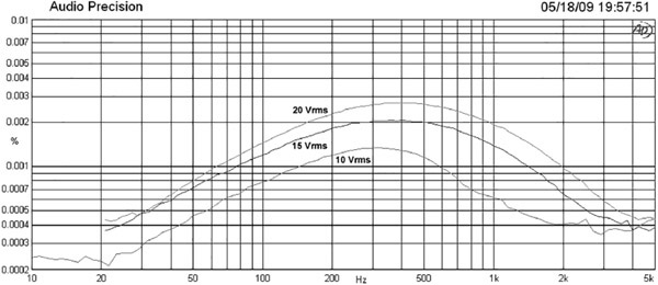
Input level Vrms	Single capacitor	Series-parallel capacitors
10	0.0016 %	0.00048 %
15	0.0023 %	0.00098 %
20	0.0034 %	0.0013%

The next dielectric we will try is polystyrene. Capacitors with a polystyrene dielectric are extremely useful for some filtering and RIAA equalisation applications because they can be obtained at a 1% tolerance at up to 10 nF at a reasonable price. They can be obtained in larger sizes at an unreasonable, or at any rate much higher, price.

The distortion test results are shown in Figure 2.18 for a 4n7 2.5% capacitor; the series resistor R1 has been increased to 4.7 kΩ to keep the −3 dB point inside the audio band, and it is now at 7200 Hz. Note that the THD scale has been extended down to a subterranean 0.0001%, and if it was plotted on the same scale as Figure 2.16 it would be bumping along the bottom of the graph. Figure 2.18 in fact shows no distortion at all, just the measurement noise floor, and the apparent rise at the HF end is simply due to the fact that the output level is decreasing because of the lowpass action, and so the noise floor is relatively increasing. This is at an input level of 10 Vrms, which is about as high as might be expected to occur in normal opamp circuitry. The test was repeated at 20 Vrms, which might be encountered in discrete circuitry, and the results were the same. No measurable distortion.

The tests were done with four samples of 10nF 1% polystyrene from LCR at 10 Vrms and 20 Vrms, with the same results for each sample. This shows that polystyrene capacitors can be used with confidence; this is in complete agreement with Cyril Bateman’s findings.[13]

Having settled the issue of capacitor distortion below 10 nF, we need now to tackle it capacitor values greater than 10 nF. Polyester having proven unsatisfactory, the next most common dielectric is polypropylene, and I might as well say at once that it was with considerable relief that I found these were effectively distortion free in values up to 220 nF. Figure 2.19 shows the results for four samples of a 220 nF 250 V 5% polypropylene capacitor from RIFA. Once more the plot shows no distortion at all, just the noise floor, the apparent rise at the HF end being increasing relative noise due to the lowpass roll-off. This is also in agreement with Cyril Bateman’s findings. Rerunning the tests at 20 Vrms gave the same result—no distortion. This is very pleasing, but there is a downside. Polypropylene capacitors of this value and voltage rating are physically much larger than the commonly used 63 or 100V polyester capacitor, and more expensive.

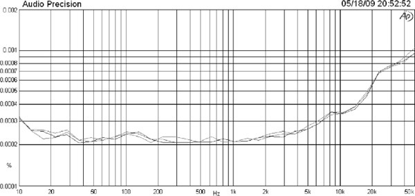
It was therefore important to find out if the good distortion performance was a result of the 250 V rating, and so I tested a series of polypropylene capacitors with lower voltage ratings from different manufacturers. Axial 47 nF 160 V 5% polypropylene capacitors from Vishay proved to be THD-free at both 10 Vrms and 20 Vrms. Likewise, microbox polypropylene capacitors from 10 nF to 47 nF with ratings of 63 V and 160 V from Vishay and Wima proved to generate no measurable distortion, so the voltage rating appears not to be an issue. This finding is particularly important because the Vishay range has a 1% tolerance, making them very suitable for precision filters and equalisation networks. The 1% tolerance is naturally reflected in the price.

The only remaining issue with polypropylene capacitors is that the higher values (above 100 nF) appear to be currently only available with 250 V or 400 V ratings, and that means a physically big component. For example, the EPCOS 330 nF 400 V 5% part has a footprint of 26 mm by 6.5 mm, with a height of 15 mm. One way of dealing with this is to use a smaller capacitor in a capacitance multiplication configuration, so a 100 nF 1% component could be made to emulate 470 nF. It has to be said that the circuitry for this is only straightforward if one end of the capacitor is connected to ground.

When I first started looking at capacitor distortion, I thought that the distortion would probably be lowest for the capacitors with the highest voltage rating. I therefore tested some RF-suppression X2 capacitors rated at 275 Vrms, which translates into a peak or DC rating of 389 V. These are designed to be connected directly across the mains and therefore have a thick and tough dielectric layer. For some reason manufacturers seem to be very coy about saying exactly what the dielectric material is, normally describing the layers simply as “film capacitors”. A problem that surfaced immediately is that the tolerance is 10 or 20%, not exactly ideal for precision filtering or equalisation. A more serious problem, however, is that they are far from distortion free. Four samples of a 470 nF X2 capacitor showed THD between 0.002% and 0.003% at 10 Vrms. Clearly a high-voltage rating alone does not mean low distortion.

Electrolytic Capacitor Nonlinearity

Cyril Bateman’s series in Electronics World[14] included two articles on electrolytic capacitor distortion. It proved to be a complex subject, and many long-held assumptions (such as “DC biasing always reduces distortion”) were shown to be quite wrong. Distortion was in general a good deal higher than for nonelectrolytic capacitors.

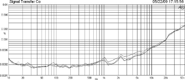
My view is that electrolytics should never, ever, under any circumstances, be used to set time-constants in audio. There should be a time-constant early in the signal path, based on a nonelectrolytic capacitor, that determines the lower limit of the bandwidth, and all the electrolytic-based time-constants should be much longer so that the electrolytic capacitors can never have significant signal voltages across them and so never generate measurable distortion. There is of course also the point that electrolytics have large tolerances and cannot be used to set accurate time-constants anyway.

However, even if you obey this rule, you can still get into deep trouble. Figure 2.20 shows a simple highpass test circuit designed to represent an electrolytic capacitor in use for coupling or DC blocking. The load of 1 KΩ is the sort of value that can easily be encountered if you are using low-impedance design principles. The calculated −3 dB roll-off point is 3.38 Hz, so the attenuation at 10 Hz, at the very bottom of the audio band, will be only 0.47 dB; at 20 Hz it will be only 0.12 dB, which is surely a negligible loss. As far as frequency response goes, we are doing fine. But … examine Figure 2.21, which shows the measured distortion of this arrangement. Even if we limit ourselves to a 10 Vrms level, the distortion at 50 Hz is 0.001%, already above that of a good opamp. At 20 Hz it has risen to 0.01%, and by 10 Hz a most unwelcome 0.05%. The THD is increasing by a ratio of 4.8 times for each octave fall in frequency, in other words increasing faster than a square law. The distortion residual is visually a mixture of second and third harmonic, and the levels proved surprisingly consistent for a large number of 47 uF 25 V capacitors of different ages and from different manufacturers.

Figure 2.21 also shows that the distortion rises rapidly with level; at 50 Hz going from an input of 10 Vrms to 15 Vrms almost doubles the THD reading. To underline the point, consider Figure 2.22, which shows the measured frequency response of the circuit with 47 uF and 1 KΩ; note the effect of the capacitor tolerance on the real versus calculated response. The roll-off that does the damage, by allowing an AC voltage to exist across the capacitor, is very modest indeed, less than 0.2 dB at 20 Hz.

Having demonstrated how insidious this problem is, how do we fix it? Changing capacitor manufacturer is no help. Using 47 uF capacitors of higher voltage does not work—tests showed there is very little difference in the amount of distortion generated. An exception was the subminiature style of electrolytic, which was markedly worse.

The answer is simple—just make the capacitor bigger in value. This reduces the voltage across it in the audio band, and since we have shown that the distortion is a strong function of the voltage across the capacitor, the amount produced drops more than proportionally. The result is seen in Figure 2.23, for increasing capacitor values with a 10 Vrms input.

Replacing C1 with a 100uF 25V capacitor drops the distortion at 20 Hz from 0.0080% to 0.0017%, an improvement of 4.7 times; the voltage across the capacitor at 20 Hz has been reduced from 1.66 Vrms to 790 mV rms. A 220 uF 25 V capacitor reduces the voltage across itself to 360 mV and gives another very welcome reduction to 0.0005% at 20 Hz, but it is necessary to go to 1000 uF 25 V to obtain the bottom trace, which is indistinguishable from the noise floor of the AP-2702 test system. The voltage across the capacitor at 20 Hz is now only 80 mV. From this data, it appears that the AC voltage across an electrolytic capacitor should be limited to below 80 mV rms if you want to avoid distortion. I would emphasise that these are ordinary 85 °C rated electrolytic capacitors and in no sense special or premium types.

This technique can be seen to be highly effective, but it naturally calls for larger and somewhat more expensive capacitors, and larger footprints on a PCB. This can be to some extent countered by using capacitors of lower voltage, which helps to bring back down the CV product and hence the can size. I tested 1000 uF 16 V and 1000 uF 6V3 capacitors, and both types gave exactly the same results as the 1000 uF 25 V part in Figure 2.23, with useful reductions in CV product and can size. This does of course assume that the capacitor is, as is usual, being used to block small voltages from opamp offsets to prevent switch clicks and pot noises rather than for stopping a substantial DC voltage.

The use of large coupling capacitors in this way does require a little care, because we are introducing a long time-constant into the circuit. Most opamp circuitry is pretty much free of big DC voltages, but if there are any, the settling time after switch-on may become undesirably long.

More information on capacitor distortion in subsonic filter applications can be found in Chapter 12.

Inductors

For several reasons, inductors are unpopular with circuit designers. They are relatively expensive, often because they need to be custom-made. Unless they are air-cored (which limits their inductance to low values) the core material is a likely source of nonlinearity. Some types produce substantial external magnetic fields, which can cause crosstalk if they are placed close together, and similarly they can be subject to the induction of interference from other external fields. Because of their series resistance they deviate from being an ideal circuit element much more than resistors or capacitors.

It is rarely, if ever, essential to use inductors in signal-processing circuitry. Historically they were used in tone controls, before the Baxandall configuration swept all before it, and their last applications were probably in mid-EQ controls for mixing consoles and in LCR filters for graphic equalisers. These too were gone by the end of the Seventies, being replaced by active filters and gyrators, to the considerable relief of all concerned (except inductor manufacturers).

The only place where inductors are essential is when the need for galvanic isolation or enhanced EMC immunity makes input and output transformers desirable, and even then they need careful handling; see Chapter 14 on line-in and line-out circuitry.

References

 1. Douglas, S. “Ultra-Low-Noise Amplifiers & Granularity Distortion” JAES, Nov 1987, pp. 907–915.

 2. Renardsen, M. www.angelfire.com/ab3/mjramp/wire. html Accessed Feb 2017.

 3. Takahisa. Nonlinearity of Resistors and Its Geometric Factor. Electronics and Communications in Japan, Volume 56-C, #6, 1973.

 4. Wikipedia https://en.wikipedia.org/wiki/Monte_Carlo_method Accessed Feb 2017.

 5. Smith, W. J. Modern Optical Engineering. McGraw-Hill, 1990, p. 484. ISBN0-07-059174-1.

 6. Johnson, H. www.edn.com/electronics-blogs/signal-integrity/4363408/7-solution Accessed Feb 2017.

 7. Kroeze, H. www.rfglobalnet.com/forums/Default.aspx?g=posts&m=61096 Accessed Mar 2002.

 8. Self, D. Audio Power Amplifier Design. 6th edition. Newnes, 2013, pp. 39–45 (voltage coeff). ISBN 978-0-240-52613-3.

 9. Self, D. Audio Power Amplifier Design. 6th edition. Newnes, 2013, p. 107 (amp output cap).

10. Bateman, C. Capacitor Sound? Parts 1–6. Electronics World, July 2002–Mar 2003.

11. Self, D. Capacitor Sound? Parts 1–6. Electronics World, July 2002–Mar 2003, p. 299 (COG cap).

12. Self, D. “Self-Improvement for Capacitors” Linear Audio, Volume 1, Apr 2011, p. 156. ISBN 9–789490–929022.

13. Bateman, C. Capacitor Sound? Part 3. Electronics World, Oct 2002, p. 16, 18.

14. Bateman, C. Capacitor Sound? Part 4. Electronics World, Nov 2002, p. 47.