Chapter 13
Ultrasonic and Scratch Filtering
Ultrasonic Filters
Scratches and groove debris create clicks that have a large high-frequency content, some of it ultrasonic and liable to cause slew rate and intermodulation problems further down the audio chain. The transients from scratches can easily exceed the normal signal level. It is often considered desirable to filter this out as soon as possible (though of course some people are only satisfied with radio-transmitter frequency responses).
If an MM input stage is provided with an HF correction pole, in the form of an RC 1st-order roll-off after the opamp, this in itself provides some protection against ultrasonics because its attenuation continues to increase with frequency and it is inherently linear. The opamp ahead of it naturally does not benefit from this; while it might be desirable to put some ultrasonic filtering in front of the first active stage, it is going to be very hard to do this without degrading the noise performance.
An ultrasonic filter could be a passive LC design, but inductors are not much loved in audio. A more likely choice is a 2nd- or 3rd-order active filter, probably opamp-based, but if Sallen and Key filters are used then a discrete emitter-follower is an option, and this should be free from the bandwidth and slew rate limitations of opamps. If an ultrasonic filter is incorporated it is usually 2nd-order, very likely due to misplaced fears of perceptible phase effects at the top of the audio band. If a Sallen and Key filter with an opamp is used, be aware that the response does not keeping going down forever but comes back up due to the nonzero output impedance of the opamp at high frequencies; the multiple-feedback (MFB) filter configuration is free from this problem.
Butterworth lowpass filters are popular for this work because their maximal flatness in the passband and rapid roll-off causes minimal intrusion into the audio band, though naturally this depends on the cutoff frequency chosen. The other important filter types are Bessel and linear-phase. As in the subsonic filter case, Bessel ultrasonic filters give a much slower roll-off as the price for keeping the group delay more constant. There seems to be a vague general feeling that phase issues are more audible at the top end of the audio band than the bottom. If you feel this is the case (and all the evidence is that it is not), you may want to use the Bessel filter characteristic. Linear-phase filters provide a compromise between the Butterworth and Bessel characteristics.
Chebyshev filters are not likely to be useful here as they introduce ripples into the passband frequency response. Elliptical filters are more complicated, and while they make excellent subsonic filters, they are not likely to be necessary for ultrasonic filtering because, unlike subsonic filters, there is usually no need for very high attenuation just outside the audio band.
Butterworth Filters from 2nd- to 6th-Order
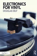
Figure 13.1 shows the circuits for Butterworth lowpass filters from 2nd-order to 6th-order; their frequency responses are shown in Figure 13.2. In each case the cutoff (−3 dB) frequency is 50 kHz, which I think gives a good compromise between passband flatness, fast roll-off, and filter complexity. For audio band flatness, the worst case is the 2nd-order Butterworth, which when designed for −3 dB at 50 kHz is only 0.11 dB down at 20 kHz. This is not much, but if you are specifying an overall frequency response of ±0.1 dB, then all of that tolerance and more is used up without considering any other part of the system. On moving to the 3rd-order Butterworth, the response droop at 20 kHz is reduced to 0.02 dB, only a fifth of the specified tolerance. The 4th-order Butterworth droop is only 0.004 dB down at 20 kHz, and for the 5th- and 6th-order Butterworths it is negligible. Considering this, it is doubtful if anything more complicated than 4th-order filter will be required, but 5th- and 6th-order filters are here if you need them. Other cutoff frequencies can be obtained by scaling the resistor values.
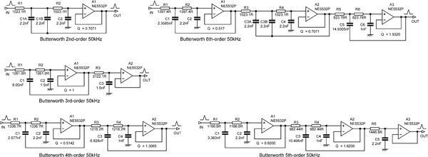
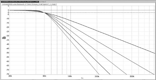
Figure 13.1 gives the component values for Butterworth filters; Tables 13.1 to 13.5 give the component values for Butterworth, linear-phase 0.5°, and Bessel ultrasonic filters, all with a cutoff frequency of 50 kHz.
A simple test that the 4th-order Bessel filter is working correctly is to check for −25 dB at three times the cutoff frequency.
The filters are made in the conventional way as a chain of second- and (sometimes) 1st-order stages. This process in covered in detail at the start of Chapter 12. The capacitor values have been chosen to keep the series resistors roughly equal to 1 kΩ, to minimise Johnson noise, the effect of current noise, and common-mode distortion without putting excessive loading on a preceding stage.
The opamps are shown as 5532/2. It is not advisable to use TL072 or similar opamps with poor gain-bandwidth product, as this will have two adverse effects:
- 1) There will be unwanted peaking of the response just before roll-off. In the case of the 6th-order filter, this will be as high as +0.5 dB around 35 kHz. If 5534 opamp models are used, this peaking is entirely absent and the proper Butterworth response is obtained.
- 2) The response will cease falling and start to come up again, above approx 300 kHz. In the 2nd-order filter it has risen back up to −30 dB at 1 mHz. If 5534 opamp models are used, the response never comes back up again.
There are no equivalent problems with subsonic filters.
Table 13.2 Resistor values for 3rd-order 50 kHz ultrasonic filter in 2xE24 format
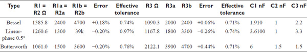
The capacitor ratio in the first stage is 4:1, so C1 can be made up exactly from four C2 capacitors in parallel; only one value is used and purchasing simplified.
Table 13.3 Resistor values for 4th-order 50 kHz ultrasonic filter in 2xE24 format
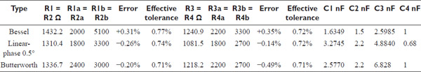
Neither of the two capacitor ratios are integers for any of the three filter types, so C1 and C3 will have to be made up with parallel capacitors. How this is best done is determined very much by what capacitor values are available. An E6 capacitor series will require much more paralleling than an E12 series. The same considerations apply to the 5th-order and 6th-order filters.
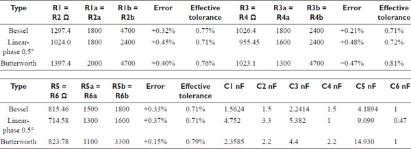
Table 13.4 Resistor values for 5th-order 50 kHz ultrasonic filter in 2xE24 format

There are no equivalent problems with subsonic filters.
Figure 13.3 compares the responses of 2nd-order Butterworth, linear-phase 0.5°, and Bessel ultrasonic filters, showing how the linear-phase characteristic chosen (0.5°) offers a good compromise between the Butterworth and Bessel characteristics. The opamp models used were 5534A; use of TL072 models gives responses that only fall to about −30 dB before coming back up again.

The component values for the three filter characteristics are shown in Table 13.6. Different cutoff frequencies can be obtained by scaling the component values, keeping the two resistors the same value and the ratio between the capacitors the same.
Combining Subsonic and Ultrasonic Filters in One Stage
An obstacle to the inclusion of an ultrasonic filter is the extra cost and power consumption of another filter stage. This difficulty can be resolved by combining it with a subsonic filter in the same stage. Combined filters also have the advantage that the signal now passes through one opamp rather than two and can be extremely useful if you only have one opamp section left. The combination of a subsonic filter and an ultrasonic filter is sometimes called a bandwidth definition filter.

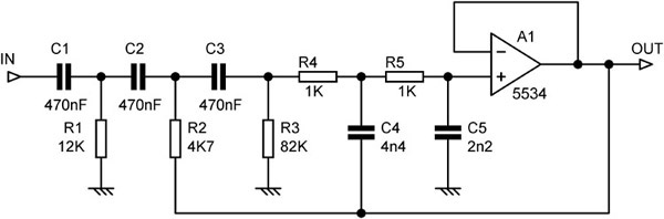
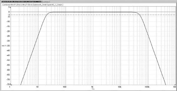
This cunning plan is workable only because the highpass and lowpass turnover frequencies are widely different. Figure 13.4 shows the 3rd-order Butterworth subsonic filter combined with a 2nd-order 50 kHz Butterworth lowpass filter; the response of the combination is exactly the same as expected for each separately. The lowpass filter is cautiously designed to prevent significant loss in the audio band and has a −3 dB point at 50 kHz, giving very close to 0.0 dB at 20 kHz. The response is −12.6 dB down at 100 kHz and −24.9 dB at 200 kHz. C4 is made up of two 2n2 capacitors in parallel.
Note that the passband gain of the combined filter is −0.15 dB rather than exactly unity. The loss occurs because the series combination of C1, C2, and C3, together with C5, forms a capacitive potential divider with this attenuation, and this is one reason why the turnover frequencies need to be widely separated for filter combining to work. If they were closer together then C1, C2, C3 would be smaller, C5 would be bigger, and the capacitive divider loss would be greater. That is why this filter is one of the few in this book that uses 470 nF capacitors rather than 220 nF.
While this is an ingenious circuit, if I do say so myself, it occurred to me that it could be improved if designed as two combined 3rd-order filters, which could be implemented by just one amplifier so long as it can be assumed that the loading on the output is sufficiently light for R6–C6 to not be significantly affected. There is some flexibility here because an ultrasonic filter does not need to be so accurate as, say, an RIAA network, because almost everything it does is above the range of audibility. The 2nd-order part of the lowpass filter is set by C4 and C5 to a Q of 1.00, as in conventional two-stage 3rd-order filters. This as usual causes a gain peak of +0.87 dB at 35 kHz; it seems unlikely this is going to cause any headroom problems. Note that a 5534 model was used as the amplifier; a TL072 model gave the usual oh-no-it’s-coming-back-up-again behaviour above 100 kHz.
The circuit is shown in Figure 13.5. In this case I used 220 nF capacitors, and as predicted the passband attenuation was a bit greater at −0.28 dB. I think this is still small enough to be ignored and definitely saves significant money on capacitors. The frequency response with its two 18 dB/octave slopes is shown in Figure 13.6.
I was going to leave it there, but the temptation to explore a topic just a little further is irresistible. To me, anyway. The result of a bit more night thought was a 4th-order highpass combined with a 4th-order lowpass in just two stages, with each stage implementing both a 2nd-order highpass and a 2nd-order lowpass, with different Q’s in the two stages, as required for Butterworth or other filter types. All the combined filters in this section are Butterworths.


The result is shown in Figure 13.7. The passband loss is smaller than that of the previous filter, at only −0.26 dB. Most of this (−0.18 dB) occurs in the first stage due to the loading of C4 on C1 and C2; the loading effect in the second stage is less because C8 is smaller. It would be possible to scale the components R3, R4, C3, C4 to reduce the passband loss, but there seems to be no pressing need to do so. There is no gain peaking in the first stage at either LF or HF because in both cases it has low Q’s, so there will be no headroom problems.
We therefore have two 4th-order filters implemented with just two amplifiers, which I fondly believe to be a new idea. The frequency response with its two 24 dB/octave slopes is shown in Figure 13.8.
It might be worth repeating at this point that combined filters only work because the highpass and lowpass cutoff frequencies are well separated—in the case of 20 Hz and 50 kHz, by 11.3 octaves.
Scratch Filters
In what might be called the First Age of Vinyl (say, 1948 to 1983, if we restrict ourselves to microgroove records), a fully equipped preamplifier would certainly have a switchable lowpass filter, usually called, with brutal frankness, the “scratch” filter. It would have a roll-off slope of at least 12 dB/octave, faster than the 6 dB/octave maximum slope of the tone-control stage and beginning at a rather higher frequency. It was aimed at suppressing, or at any rate dulling and hopefully rendering acceptable, not just record surface noise and the inevitable ticks and clicks but also HF distortion. This function is quite separate from that of an ultrasonic filter, and the turnover frequency is very much in the audio band, usually in the range 3–10 kHz.

The more highly specified preamps would have two, three, or more alternative filter frequencies, and the really posh models had variable filter slope as well. The fact that the need was felt for some really quite sophisticated filtering to smooth the listening experience does rather emphasise the inherent vulnerability of a mechanical groove for delivering music. Now we seem to be in the Second Age of Vinyl, a reassessment of this once-abandoned bit of technology would seem to be timely.
Historically, scratch filters were often passive LC configurations, as it was much cheaper to design in a wound component than to add an extra valve to make an active filter. A modern scratch filter will almost certainly be an active filter based on one of the designs for ultrasonic filters given earlier, the only difference being that the cutoff frequency will be much lower, in the range 3 to 10 kHz, depending on just how badly the vinyl is scratched.
Fixed-frequency scratch filters from 2nd- to 6th-order can be quickly designed by modifying the ultrasonic filter designs given at the start of this chapter. The simplest way is to scale the capacitor values, keeping them in the same ratio. As an example, Figure 13.1 shows a 3rd-order Butterworth lowpass with a cutoff frequency of 50 kHz, with C1 = 6 nF, C2 = 1.5 nF, and C3 = 1.5 nF. To turn this into a 5 kHz cutoff scratch filter, the capacitors are increased by a factor of 10 times, so C1 = 60 nF, C2 = 15nF, and C3 = 15 nF. The 60 nF can be made up from four 15 nF capacitors in parallel, so only one value is used and purchasing simplified.
Variable-Frequency Scratch Filters
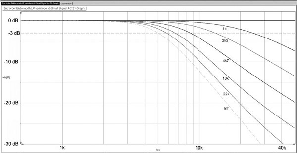
Making a variable-frequency scratch filter is relatively simple providing you are satisfied with a 2nd-order response. A lowpass 2nd-order Sallen and Key filter has two equal resistors, and these can be easily changed together with a ganged pot, though naturally this requires a 4-gang pot for stereo. Figure 13.9 shows such a filter with the wide frequency range of 1 kHz to 10 kHz. This can be reduced by increasing the value of the end-stop resistors R1, R2, and reducing C1 and C2 to keep the maximum frequency the same.
Third-order scratch filters can be made in the same way by adding a variable third pole after opamp A1; this however requires a somewhat less practical 6-gang pot.
Variable-slope scratch filters are dealt with in the next three sections. Usually the cutoff frequency and the slope are altered together.
Variable-Slope Scratch Filters: LC Solutions
Making a variable-slope filter is not that straightforward, because the natural slopes you get with resistors and capacitors are 6 dB per octave. Using active filters gives access to final slopes with 12, 18, 24, or more dB per octave, but intermediate slopes are usually only found in the transitions between flat and the ultimate roll-off slope.
A popular way of achieving variable slope back in the valve era involved an LC filter bypassed by a variable resistance. A classic example of this approach, published in Wireless World in 1956,[1] is shown in Figure 13.10. If RV1 is absent, there is a deep notch centred on 10 kHz, but adding it abolishes the notch and gives the response shown in the bottom trace of Figure 13.11.
Adjusting RV1 to steadily reduce the resistance across L1, C2 gives a set of responses that have more or less the same turnover frequency (−3 dB at about 3 kHz) but reducing slope. If we measure the average slopes across the octave 5–10 kHz, we get Table 13.7, which shows a handy variation in slope from 4.5 to almost 18 dB/octave. As revealed in Figure 13.11, the filter has 6 dB loss in the passband, which is a long way from ideal. Noise or headroom will be seriously compromised.
The full published circuit included switching of all three capacitors to give nominal turnover frequencies of 5, 7, and 10 kHz, which of course means a rather clumsy 6-pole switch for stereo use. It had a 1 H inductor, which required 1100 turns to be wound on a Ferroxcube core, so its construction required some degree of commitment. RV1 was a log-law component. This form of filter resurfaced in a transistor preamplifier design by Reg Williamson in 1967.[2]
Variable-Slope Scratch Filters: Active Solutions
The prospect of winding 1100 turns on a former to make an inductor is not at all appealing, and would turn anybody’s mind to RC active filters. This is quite apart from the well-known inductor drawbacks of weight, cost, nonlinearity, and susceptibility to hum fields. The well-known Leak Varislope preamplifiers of the 1950s used purely RC filtering, boasting specifically in their advertising material that there were no chokes to pick up hum. The earliest (mono) version had three switched filter frequencies plus “Off” and only offered two switched slope settings, “steep” and “gradual”. The later Varislope II lived up to its name better by having switched filter frequencies but fully variable slopes using a two-gang pot. Still later, the stereo versions (Gold & Grey) reverted to switched slopes, perhaps because a four-gang pot was not at the time a viable proposition. The circuitry can be found on the Web.[3]

In 1970 John Linsley-Hood published an RC variable-slope filter design,[4] but its operation was quite unacceptable, having irregularities in the passband down to 100 Hz and +3 dB of internal peaking that eroded headroom. In 1990 Reg Williamson most ingeniously converted the LC filter to a more practical form by replacing the floating inductor with two gyrators;[5] the downside was that it required five opamp sections per channel.
Bypass resistance |
Slope in dB/octave |
|---|---|
220 kΩ |
17.6 dB/oct |
100 kΩ |
11.7 dB/oct |
47 kΩ |
7.8 dB/oct |
22 kΩ |
5.7 dB/oct |
10 kΩ |
4.8 dB/oct |
0 Ω |
4.5 dB/oct |

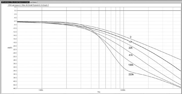
When I needed a varislope filter in 1978 I decided to have a go at designing my own version. The first attempt was adding a bypass resistance to a standard 2nd-order Butterworth Sallen and Key filter, as shown in Figure 13.12, with the response results in Figure 13.13, where the dashed bottom trace shows the pure 2nd- order Butterworth characteristic obtained when the bypass resistance is entirely absent. The slopes are indeed varying smoothly and are summarised in Table 13.8. Naturally the maximum slope is somewhat less than 12 dB/octave, since we started out with a 2nd-order filter. The turnover frequency varies with the slope, though this is not necessarily a disadvantage. We are trying to make tolerable the reproduction from a very imperfect medium, not design a laboratory instrument. Here increasing the bypass resistance gives “more filtering” in two ways because the turnover frequency is reduced as the slope is increased.
In practice, adding a 1 kΩ end-stop resistor in series with the slope pot would probably be a good idea, as this will prevent C2 being connected directly to the output of the previous stage, which may object by going unstable. It is assumed there is a way of switching out the filter stage completely.
Bypass resistance |
Slope in dB/octave |
|---|---|
None |
11.8 dB/oct |
22 kΩ |
10.5 dB/oct |
10 kΩ |
8.9 dB/oct |
4k7 |
6.9 dB/oct |
2k2 |
4.2 dB/oct |
1 kΩ |
1.7 dB/oct |
While the second-order lowpass filter with bypass resistance delivers variable slopes quite well, it is doubtful if a maximum slope of 12 dB/octave is really enough; the historical LC filter gave a maximum of almost 18 dB/octave.
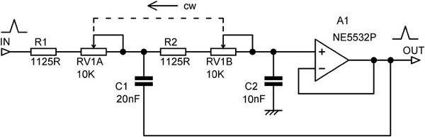
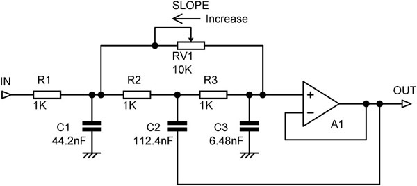
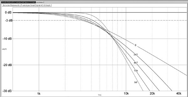
I therefore took another swing at the problem by starting with a 3rd-order Butterworth Sallen and Key filter, as in Figure 13.14. I have not converted the exact capacitor values to combinations of preferred values. Connecting a bypass resistance between the input and C3 gives no useful result, but wiring it between C1 and C3 gives the response in Figure 13.15. The operation is not the same as for the 2nd-order filter; there is something like a constant turnover frequency, but this does not align with the dashed line at −3 dB; rather it occurs around −7 dB. A variable-slope characteristic is obtained with slopes of between 5 and 15 dB/octave, as summarised in Table 13.9.
There is now no need to add an end-stop resistor in series with the slope pot, as C3 is never connected directly to the input. I am not claiming that these bypass filters are the last word on the subject, but they are certainly more economical of parts than the Williamson gyrator filter. To the best of my knowledge this is the first time this technique has been published.
Bypass resistance |
Slope in dB/octave |
|---|---|
None |
15.2 dB/oct |
10 kΩ |
12.0 dB/oct |
4k7 |
9.4 dB/oct |
2k2 |
7.1 dB/oct |
0 Ω |
5.0 dB/oct |
Variable-Slope Scratch Filters: The Hamill Filter
If slightly different design criteria are used, a different form of variable scratch filter results. In a 1981 article in Wireless World,[6] David Hamill concluded that lowpass filters with rapid roll-offs around the cutoff frequency introduced colouration, but this could be avoided if the area around cutoff had a slow roll-off to prevent ringing on transients. The Gaussian filter characteristic is optimised for its time response, giving no overshoot and minimum rise and fall times on edges, but it gives a slow roll-off when near the cutoff frequency. Hamill stated that making the roll-off Gaussian for the first 10 dB or so is enough to prevent ringing, but as the filter cutoff frequency increases the roll-off can be made faster as the ear becomes less sensitive to colouration. His design therefore had a variable slope around the cutoff frequency, transitioning to a fixed 18 dB/octave ultimate slope at higher frequencies, unlike the filters described earlier, which have variable ultimate slopes.
One slight problem with Gaussian filters is that they are impossible to construct. The slow roll-off that gives the good time response is obtained by cascading a series of 1st-order stages of differing and carefully chosen frequencies; the Gaussian roll-off slope steadily increases with frequency and is infinite at infinite frequency. You therefore need an infinite number of 1st-order stages, which makes construction rather difficult. It is however entirely practical to build an approximation to a Gaussian filter by keeping the slow initial roll-off but then smoothly splicing this to a constant, and therefore more practical, filter slope such as the 18 dB/octave of a 3rd-order Butterworth or Bessel filter. All real “Gaussian” filters are therefore actually transitional filters.
The original published design included a fixed-frequency 3rd-order subsonic filter, but its presence or absence does not affect the operation of the scratch filter, and it is omitted here for clarity. The filter very cleverly has only one control to set cutoff frequency and slope around cutoff. As the control is turned the cutoff frequency increases, and at the same time the slope around the cutoff increases, the filter characteristic moving from a Bessel approximation to a Gaussian filter, through Butterworth, to a Chebyshev response with 0.5 dB passband ripple. This single “ripple” is a very shallow peak around 15 kHz and is highly unlikely to be perceptible. The control is a single pot making stereo operation with a dual-gang pot simple. I think we should call this a Hamill filter.
My interpretation of this filter is shown in Figure 13.16. The basic configuration is that of a two-stage 3rd-order Sallen and Key filter, with 2nd-order stage around A2, but the innovation is that capacitors C2 and C4 are driven by a scaled version of the output voltage. The scaling factor is set by RV1, with R6 bending the control law so it approximates to logarithmic, i.e. linear in octaves. The circuit impedances have been reduced by a factor of 4.25 to improve the noise performance with modern opamps (the original design used discrete transistors), the precise factor being chosen to make the largest capacitor C3 exactly 20 nF, so it can be made from two 10 nF polystyrene capacitors C3A, C3B in parallel. This luckily gave a value of almost exactly 1.2 kΩ for R1, R2, and R3. The other capacitors, C1, C2, and C4, inevitably have awkward values; they are made up assuming only E6 series components are available. As luck would have it, C1 and C4 come out very nicely, their combined nominal values being within 0.1% of the target, though three parallel capacitors, C4A, C4B, and C4C, are required to achieve this for C4. C2 is a bit less favourable, coming out 1% high, but this seems to have very little effect on the responses, which as far as the eye can judge are identical to those published in Wireless World.
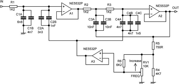

The frequency responses for four control settings as the pot wiper is moved upwards are shown in Figure 13.17, and it can be seen that the Hamill filter does its work most effectively and ingeniously. It should prove useful for archival transcription work.
References
1. Leakey, D. “Inexpensive Variable-Slope Filter” Wireless World, Nov 1956, p. 563.
2. Williamson, R. “All-Silicon Transistor Stereo Control Unit” Hi-Fi News, May 1967.
3. www.44bx.com/leak/leak_ccts.html Accessed Nov 2016.
4. Linsley-Hood, J. “Modular Pre-amplifier Design Postscript” Wireless World, Dec 1970, p. 609.
5. Williamson, R. “Variable-Slope Lowpass LF Filter” Wireless World, Aug 1990, p. 714.
6. Hamill, D. “Transient Response of Audio Filters” Wireless World, Aug 1981, p. 59.