C H A P T E R 13
Essentials for Effective Coding
Now that you know how to build and work with SQL Server objects, and insert, update, and delete data as well as retrieve it, you can move on to more of the T-SQL essentials required to complete your programming knowledge.
Potentially, the most important area covered by this chapter is error handling. After all, no matter how good your code is, if it cannot cope when an error occurs, then it will be hard to keep the code stable and reliable. There will always be times that the unexpected happens, from strange input data to something happening on the server. However, this is not the only area of interest. You will be looking at methods to perform aggregations of data and grouping data together. Finally, there will be times that you want to hold data either in a variable or a table and have it exist for only a short period. This is quite a great deal to cover, but this chapter and the next will be the stepping stones that move you from novice to professional developer.
This chapter will therefore look at the following:
- Having a method of storing information temporarily using variables
- Storing rows of information in a nonpermanent table
- Aggregating values
- Organizing output data into groups of relevant information
- Returning unique and distinct values
- Looking at and using system functions
- Handling errors, e.g., creating your own errors, trapping errors, and making code secure
Variables
Sometimes you’ll need to hold a value or work with a value that does not come directly from a column. Or perhaps you’ll need to retrieve a value from a single row of data and a single column that you want to use in a different part of a query. It is possible to do this via a variable.
You can declare a variable at any time within a set of T-SQL instructions, whether it is ad hoc or a stored procedure or trigger. However, a variable has a finite lifetime.
To inform SQL Server that you want to use a variable, use the following syntax:
DECLARE @variable_name datatype[, @variable_name2 datatype]
All variables have to be preceded with an @ sign, and as you can see from the syntax, more than one variable can be declared, although multiple variables must be separated by a comma or a new line with a new DECLARE statement. Code can be held on more than one line within the editor, just like all other T-SQL syntax, such as having DECLARE on line 1 and then the variables on line 2. All variables can hold a NULL value, and there is not an option to say that the variable cannot hold a NULL value. By default, then, when a variable is declared, it will have an initial value of NULL. It is also possible to assign a value at the time of declaration. You’ll see this in the first set of the following code. To assign a value to a variable, you can use a SET statement or a SELECT statement. It is standard to use SET to set a variable value when you are not working with any tables, and it is useful when you want to set the values of multiple variables at the same time. It is also useful when you want to check the system variables @@ERROR or @@ROWCOUNT following some other DML statements. You will see these system variables later within this chapter. Let’s take a look at some examples to see more of how to work with variables and their lifetime.
TRY IT OUT: DECLARING AND WORKING WITH VARIABLES
- In this example, you define two variables; in the first, you are placing the current date and time using the system function
GETDATE(), and in the second, you are setting the value of the variable@CurrPriceInCentsto the value from a column within a table with a mathematical function tagged on. Once these two have been set usingSETandSELECT, you then list them out, which can be done only via aSELECTstatement.DECLARE @MyDate datetime=GETDATE(), @CurrPriceInCents moneyn
SELECT @CurrPriceInCents = CurrentPrice * 100
FROM ShareDetails.Shares
WHERE ShareId = 2
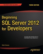
SELECT @MyDate,@CurrPriceInCents - Execute the code, and you will see something like the results shown in Figure 13-1. The first column shows your current date and time.
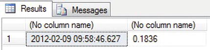
Figure 13-1. Working with a local variable
- If you change the query into two batches, the variables in the second batch will not exist, and when you try to execute all of the code at once, you will get an error. Enter the code as it appears here; the only real change is the
GOstatement, shown in bold:DECLARE @MyDate datetime= GETDATE(), @CurrPriceInCents money
SELECT @CurrPriceInCents = CurrentPrice * 100
FROM ShareDetails.Shares
WHERE ShareId = 2
GO
SELECT @MyDate,@CurrPriceInCents - The error returned when this code is executed is shown here. You are being informed that SQL Server doesn’t know about the first variable in the last statement. This is because SQL Server is parsing the whole set of T-SQL before executing, rather than one batch at a time.
Msg 137, Level 15, State 2, Line 1

Must declare the scalar variable "@MyDate".
- Remove the
GOstatement so you can see one more example of how variables work. You also need to remove theWHEREstatement in the example so that you return all rows from theShareDetails.Sharestable. The value that will be assigned to the variable@CurrPriceInCentswill be the last value returned from the query of data. The code you want to execute is as follows. The two lines have been retained in the query, but they have now been prefixed with two dashes: --. This indicates to SQL Server that the lines of code have been commented out and should be ignored.DECLARE @MyDate datetime= GETDATE(), @CurrPriceInCents money
SELECT @CurrPriceInCents = CurrentPrice * 100
FROM ShareDetails.Shares
--WHERE ShareId = 2
--GO
SELECT @MyDate,@CurrPriceInCents - If you look at the results that this produces, as shown in Figure 13-2, you can see that the value in the second column is from the last row in the
ShareDetails.Sharestable, which could also be found by performingSELECT TOP 1 * FROM ShareDetails.Shares ORDER BY ShareId DESC.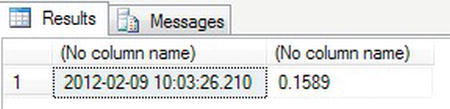
Figure 13-2. Variables and batches
![]() Note Recall from previous chapters that the query as detailed in step 4 will retrieve a value in any order; it will not necessarily be the last row inserted into the table.
Note Recall from previous chapters that the query as detailed in step 4 will retrieve a value in any order; it will not necessarily be the last row inserted into the table.
Temporary Tables
There are two types of temporary tables: local and global. These temporary tables are created in tempdb and not within the database you are connected to. They also have a finite lifetime. Unlike a variable, the time such a table can “survive” is different.
- A local temporary table survives until the connection it was created within is dropped. This can happen when the stored procedure that created the temporary table completes, or when the Query Editor window is closed. A local temporary table is defined by prefixing the table name by a single hash mark: #. The scope of a local temporary table is the connection that created it only.
- A global temporary table is defined by prefixing the table name by a double hash mark: ##. The scope of a global temporary table differs significantly. When a connection creates the table, it is then available to be used by any user and any connection, just like a permanent table. A global temporary table will then be “deleted” only when all connections to it have been closed.
In Chapter 10, when looking at the SELECT statement, you were introduced to SELECT...INTO, which allows a permanent table to be built from data from either another table or tables, or from a list of variables. You could make this table more transient by defining the INTO table to reside within tempdb. However, it will still exist within tempdb until either it is dropped or SQL Server is stopped and restarted. This is slightly better, but not perfect for when you just want to build an interim table between two sets of T-SQL statements.
Requiring a temporary table could happen for a number of reasons. Building a single T-SQL statement returning information from a number of tables can get complex, and perhaps could even not be ideally optimized for returning the data quickly. Splitting the query into two may make the code easier to maintain and perform better. To give an example, as your customers “age,” they will have more and more transactions against their account IDs. It may be that when working out any interest to accrue, the query will take a long time to run, as there are more and more transactions. It might be better to create a temporary table of just the transactions you are interested in, and then use this temporary table in code that then calculates the interest, rather than trying to complete all the work in one pass of the data.
When it comes time to work with a temporary table, such a table can be built either by using the CREATE TABLE statement or by using the SELECT...INTO command. From a performance perspective, you will find defining a temporary table and then populating it faster than a SELECT…INTO. If you define a table, SQL Server will know each column’s data type from the definition; however, with a SELECT…INTO, SQL Server has to calculate what data each column holds from the data and then decide on the data type. Let’s take a look at temporary tables in action.
TRY IT OUT: TEMPORARY TABLES
The first example will create a local temporary table based on the CREATE TABLE statement. You will populate the table with some data and retrieve the data. You will then open up a different Query Editor pane and try to retrieve data from the table to show that it is local. Also of interest here is how you can use a SELECT statement in conjunction with an INSERT statement to add the values. Providing that the number of columns returned in the SELECT matches either the number of columns within the table or the number of columns in the INSERT column list, using a SELECT statement is a great way of populating tables, especially temporary tables.
- First, create the temporary table. For the moment, just enter the code; don’t execute it.
CREATE TABLE #SharesTmp

(ShareDesc varchar(50),

Price numeric(18,5),

PriceDate datetime) - Next, you want to populate the temporary table with information from the
ShareDetails.Sharesand theShareDetails.SharePricestables. Because you are populating every column within the table, you don’t need to list the columns in theINSERT INTOtable part of the query. Then, you use the results from aSELECTstatement to populate many rows in one set of T-SQL. You can execute the code now if you want, but when you get to the third part in a moment, run theSELECT *from the same Query Editor window.INSERT INTO #SharesTmp
SELECT s.Description,sp.Price,sp.PriceDate
FROM ShareDetails.Shares s
JOIN ShareDetails.SharePrices sp ON sp.ShareId = s.ShareId - The final part is to prove that there are data in the table.
SELECT * FROM #SharesTmp - When the code is executed, you should see the output that appears in Figure 13-3.
Figure 13-3. A local temporary table
- Open up a fresh Query Editor, keeping the current connection and Query Editor open, and then try to execute the following code:
SELECT * FROM #SharesTmp - Now instead of returning a set of results like those shown in Figure 13-3, you will get an error message similar to that here. This is because the temporary table is a local temporary table and is available only from the connection that created it.
Msg 208, Level 16, State 0, Line 1

Invalid object name '#SharesTmp'.
- If you change the whole query to now work with a global temporary variable, you will see a different end result. To ensure you are starting afresh, clear all the Query Editors, or execute the following
DROP TABLEcommand in the first Query Editor:DROP TABLE #SharesTmp Note It is good practice to
 DROPa temporary table when you have finished using it rather than letting SQL Server drop the table when the connection closes. If you leave Query Editor open, then the temporary table will continue to exist intempdb. If you generate one or more large temporary tables, you can find that you have notempdbdatabase space left and your database will stop processing when it requires space intempdbto perform some work. - Enter the following code, taking note of the double hash marks, in one of the Query Editors:
CREATE TABLE ##SharesTmp
(ShareDesc varchar(50),
Price numeric(18,5),
PriceDate datetime)
INSERT INTO ##SharesTmp
SELECT s.Description,sp.Price,sp.PriceDate
FROM ShareDetails.Shares s
JOIN ShareDetails.SharePrices sp ON sp.ShareId = s.ShareId SELECT * FROM ##SharesTmp - When you execute the code, you should see the same results as you did with the first query (refer back to Figure 13-3).
- Move to a new Query Editor, ensuring that you leave the previous Query Editor pane still open. Then enter the following
SELECTstatement:SELECT * FROM ##SharesTmp - When this is executed, you see the same results again, as shown originally in Figure 13-3.
It is not until the first Query Editor pane that defined the global table is closed or until a DROP TABLE ##SharesTmp is executed that the table will disappear.
Aggregations
An aggregation is where SQL Server performs a function on a set of data to return one aggregated value per grouping of data. This will vary from counting the number of rows returned from a SELECT statement through to figuring out maximum and minimum values. Combining some of these functions with the DISTINCT function, discussed later in the “Distinct Values” section, can provide some useful functionality. An example might be when you want to show the highest value for each distinct share to demonstrate when the share was worth the greatest amount.
Let’s dive straight in by looking at different aggregation types and working through examples of each.
COUNT/COUNT_BIG
COUNT/COUNT_BIG is probably the most commonly used aggregation, and it finds out the number of rows returned from a query. You use this for checking the total number of rows in a table, or more likely the number of rows returned from a particular set of filtering criteria. Quite often this is used to cross-check the number of rows from a query in SQL Server with the number of rows an application is showing to a user.
The syntax is COUNT(*) or COUNT_BIG(*). There are no columns defined, as it is rows that are being counted.
![]() Note The difference in these two functions is that
Note The difference in these two functions is that COUNT returns an integer data type, and COUNT_BIG returns a bigint data type.
TRY IT OUT: COUNTING ROWS
- This example will count the number of rows in the
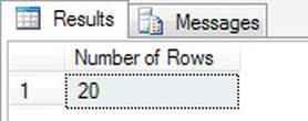
Sharestable. In the example, you will see an asterisk between the brackets. This is the normal method, although you could have a number or a column; however, I find these confusing. There is no performance difference. You will likely find that you useCOUNTeither to ensure a table has the number of rows you expect, or to populate a variable. If you find you are returning the count as a result set outside of a stored procedure, you should name the column with an alias, as demonstrated in the example:SELECT COUNT(*) AS 'Number of Rows'
FROM ShareDetails.Shares - Execute the code, and you will see the results shown in Figure 13-4.
- Of course, you could add a filter such as the following, which counts the number of customers who do not have an uncleared balance pending to clear.
SELECT COUNT_BIG(*) AS 'Number of Rows'

FROM CustomerDetails.Customers

WHERE UnclearedBalance IS NULL - Execute the code, and you will now see a count of 710, shown in Figure 13-5, as expected.
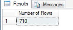
Figure 13-5.
COUNT_BIGwith a filter
SUM
If you have numeric values in a column, it is possible to aggregate them into a sum. One scenario for this is to add the transaction amounts in a bank account to see how much the balance has changed by. This could be daily, weekly, monthly, or over any time period required. For example, a negative amount would show that more has been taken out of the account than put in.
The syntax can be shown as SUM(column1|@variable|Mathematical function). The summation does not have to be of a column, but could include a math function. One example would be to sum up the cost of purchasing shares, so you would multiply the number of shares bought by the cost paid.
TRY IT OUT: SUMMING VALUES
- You can do a simple
SUMto add up the amount of money that has passed through the account as a deposit. The transaction type for this from theTransactionDetails.Transactionstable is where the columnTransactionTypehas a value of 1.SELECT SUM(Amount) AS 'Amount Deposited'
FROM TransactionDetails.Transactions
WHERE CustomerId = 1
AND TransactionType = 1 - Executing this code adds up two rows you inserted for customer 1. The results are 175.67, as shown in Figure 13-6.
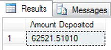
Figure 13-6.
SUMming values
MAX/MIN
On a set of data, it is possible to get the minimum and maximum values of a column of data. This is useful if you want to see values such as the smallest share price or the greatest portfolio value, or in other scenarios outside of the example, as the maximum number of sales of each product in a period of time, or the minimum sold, so that you can see if some days are quieter than others.
TRY IT OUT: MAX AND MIN
- In this example, you will see how to find the maximum and minimum values for a share with one statement. Enter the following code:
SELECT MAX(Price) MaxPrice,MIN(Price) MinPrice

FROM ShareDetails.SharePrices

WHERE ShareId = 1 - Executing the code produces the results shown in Figure 13-7.
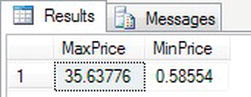
Figure 13-7. Find the maximum and minimum
AVG
As you might expect, the AVG aggregation returns the average value of a column of data for the filtered rows. All of the values are added and then divided by the number of rows that formed the underlying result set.
TRY IT OUT: AVERAGING IT OUT
- The last aggregation example will produce an average value for the share prices found for share ID 1. Enter the following code:
SELECT AVG(Price) AvgPrice

FROM ShareDetails.SharePrices

WHERE ShareId = 1 - Once you have executed the code, you should see the results shown in Figure 13-8.
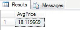
Figure 13-8. Finding the average
Now that you have taken a look at aggregations, you can move on to looking at grouping data. Aggregations, as you have seen, are useful but limited. In the next section, I will show you how you can expand these aggregations so that they are used with groups of data.
Grouping Data
Using aggregations works well when you want just a single row of results for a specific filtered item. If you want to find the average price of several shares, you may be thinking you need to provide a SELECT AVG() for each share. This section will demonstrate that this is not the case. By using GROUP BY, you instruct SQL Server to group the data to return and provide a summary value for each grouping of data. To clarify, as you will see in the upcoming examples, you could remove the WHERE ShareId=1 statement, which would then allow you to group the results by each different ShareId. In Chapter 14, where you will look at more advanced T-SQL, you will see how it is possible to create more than one grouped set. For the moment, though, let’s keep it straightforward.
The basic syntax for grouping follows. (It is possible to expand GROUP BY further to include rolling up or providing cubes of information, which, as part of grouping sets, you will see in Chapter 14.)
GROUP BY [ALL] (column1[,column2,...])
The option ALL is a bit like an OUTER JOIN. If you have a WHERE statement as part of your SELECT statement, any grouping filtered out will still return a row in the results, but instead of aggregating the column, a value of NULL will be returned. I tend to use this as a checking mechanism. I can see the rows with values and the rows without values, and visually this will tell me that my filtering is correct.
When working with GROUP BY, the main point that you have to be aware of is that any column defined in the SELECT statement that does not form part of the aggregation must be contained within the GROUP BY clause and be in the same order as the SELECT statement. Failure to do this will mean that the query will give erroneous results, and in many cases, will use a lot of resources in giving these results.
TRY IT OUT: GROUP BY
- This first example will demonstrate how to find maximum and minimum values for every share that has a row in the
ShareDetails.SharePricestable where the shareDescriptionis greater than Julies Pantry. The code is as follows:SELECT sp.ShareId, s.Description,MIN(Price) MinPrice, Max(Price) MaxPrice
FROM ShareDetails.SharePrices sp
LEFT JOIN ShareDetails.Shares s ON s.ShareId = sp.ShareId
WHERE s.Description > 'Julies Pantry'
GROUP BY sp.ShareId, s.Description - When the code is executed, you will see the 11 shares listed with their corresponding minimum and maximum values, as shown in Figure 13-9.
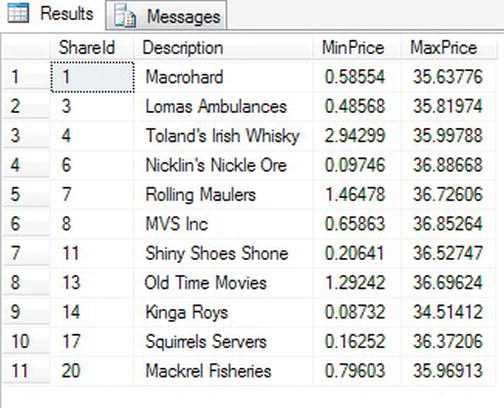
Figure 13-9. Max and min of a group
- If you want to include all rows where there is no
Price, as it has been removed by theWHEREclause, then you would use theALLoption withGROUP BY:SELECT sp.ShareId, s.Description,MIN(Price) MinPrice, Max(Price) MaxPrice
FROM ShareDetails.SharePrices sp
LEFT JOIN ShareDetails.Shares s ON s.ShareId = sp.ShareId
WHERE s.Description > 'Julies Pantry'
GROUP BY ALL sp.ShareId, s.Description - When you execute the code, the
Pricerow that is outside of the filtering returns aNULLvalue. The other rows return details as shown in Figure 13-10.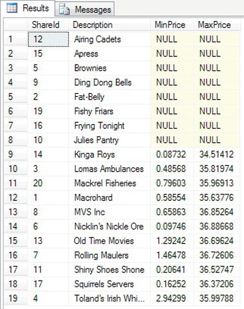
HAVING
When using the GROUP BY clause, it is possible to supplement your query with a HAVING clause. The HAVING clause is like a filter, but it works on aggregations of the data rather than the rows of data prior to the aggregation. Hence, it has to be included with a GROUP BY clause. It will also include the aggregation you want to check. The code would therefore look as follows:
GROUP BY column1[,column2...]

HAVING [aggregation_condition]
The aggregation_condition would be where you place the aggregation and the test you want to perform. For example, my bank charges me if I have more than 20 nonregular items pass through my account in a month. In this case, the query would group by customer ID, counting the number of nonregular transactions for each calendar month. If the count were less than or equal to 20 items, then you would like this list to not include the customer in question. To clarify this, the query code would look something like the following if you were running this in August 2011:
SELECT CustomerId,COUNT(*)

FROM CustomerBankTransactions

WHERE TransactionDate BETWEEN '1 Aug 2011' AND '31 Aug 2011 '

GROUP BY CustomerId

HAVING COUNT(*) > 20
TRY IT OUT: HAVING
- In the following example, you will use the
MINaggregate function to remove rows where the minimum share price is less than $10. This query is taken from theGROUP BY ALLexample shown earlier. Although you have kept theALLoption within theGROUP BYstatement, it is ignored, as it is followed by theHAVINGclause.SELECT sp.ShareId, s.Description,MIN(Price) MinPrice, Max(Price) MaxPrice
FROM ShareDetails.SharePrices sp
LEFT JOIN ShareDetails.Shares s ON s.ShareId = sp.ShareId
WHERE s.Description > 'Julies Pantry'
GROUP BY ALL sp.ShareId, s.Description
HAVING MIN(Price) < 10 - The results on the executed code will return 11 values, as you see in Figure 13-11, ignoring the shares that have a
MinPricevalue ofNULLthat would be returned by theALL.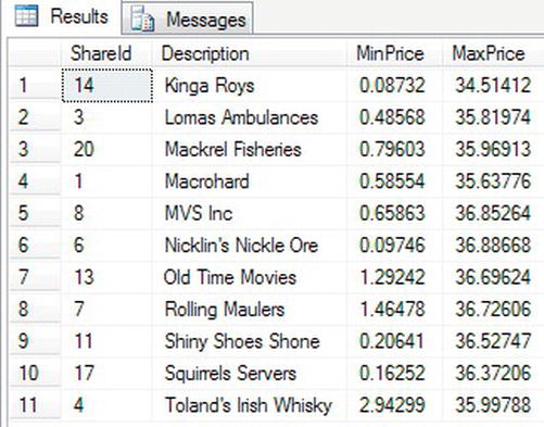
Figure 13-11. When you want to have only certain aggregated rows
Even if you changed the HAVING to being greater than $10, the shares with a Description of less than or equal to Julies Pantry would still be ignored due to the HAVING overriding the GROUP BY ALL. Not only that, but also NULL, as you know, is a “special” value and is neither less than nor greater than any value.
Distinct Values
With some of the tables in the examples, multiple entries will exist for the same value. To clarify, in the ShareDetails.SharePrices table, there can be multiple entries for each share as each new price is stored. There may be some shares with no price, of course. But what if you want to see a listing of shares that do have prices, but you want to see each share listed only once? This is a simple example, and you will see more complex examples later on when I cover how to use aggregations within SQL Server. That aside, the example that follows serves its purpose well.
The syntax is to place the keyword DISTINCT after the SELECT statement and before the list of columns. The following list of columns is then tested for all the rows returned, and for each set of unique distinct values, one row will be listed.
TRY IT OUT: DISTINCT VALUES
- You have to join the
ShareDetails.SharesandShareDetails.SharePricestables again so that you know you are returning only rows that have a share price. You had that code in yourJOINsection earlier in the chapter in step 2 of the “Temporary Tables” exercise. It is replicated here, and you can execute it if you want:SELECT s.Description,sp.Price,sp.PriceDate
FROM ShareDetails.Shares s
JOIN ShareDetails.SharePrices sp ON sp.ShareId = s.ShareId - As you know, this returns multiple rows for each share. Placing
DISTINCTat the start of the column list doesn’t make any difference, because there are different prices and different price dates.SELECT DISTINCT s.Description,sp.Price,sp.PriceDate
FROM ShareDetails.Shares s
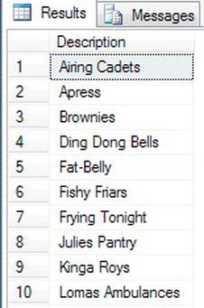
JOIN ShareDetails.SharePrices sp ON sp.ShareId = s.ShareId - To get a list of shares that have a value, it is necessary to remove the last two columns and list only the
ShareDesccolumn.SELECT DISTINCT s.Description
FROM ShareDetails.Shares s
JOIN ShareDetails.SharePrices sp ON sp.ShareId = s.ShareId - When you execute this code, you will see the desired results, as partly shown in Figure 13-12.
Functions
To bring more flexibility to your T-SQL code, you can use a number of functions with the data from variables and columns. This section does not include a comprehensive list, but it does contain the most commonly used functions and the functions you will come across early in your development career. They have been split into three categories: date and time, string, and system functions. There is a short explanation for each, with some code demonstrating each function in an example with results.
Date and Time
The functions in the first set involve either working with a variable that holds a date and time value or using a system function to retrieve the current date and time.
DATEADD()
If you want to add or subtract an amount of time to a column or a variable, then display a new value in a rowset or set a variable with that new value; DATEADD() will do this. The syntax for DATEADD() is as follows:
DATEADD(datepart, number, date)
The datepart option applies to all of the date functions and details what you want to add from milliseconds to years. These are defined as reserved words and therefore are not surrounded by quotation marks. There are a number of possible values, as listed in Table 13-1.
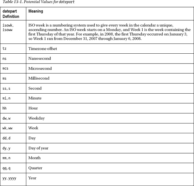
For the second parameter of the datepart function, to add, use a positive value, and to subtract, use a negative value. The final parameter can be a value, a variable, or a date-type column holding the date and time you want to change.
TRY IT OUT: DATEADD()
- In this example, you will set a local variable to a date and time. Once the variable is set, you will add four hours to the value and display the results. Enter the code here, and then execute it, which should return results as shown in Figure 13-13.
DECLARE @OldTime datetime

SET @OldTime = '24 March 2012 3:00 PM'

SELECT DATEADD(hh,4,@OldTime)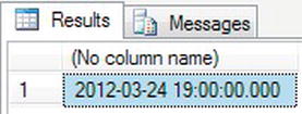
Figure 13-13. Adding hours to a date
- Taking the reverse, you will take the same variable and subtract six hours. The results should appear as shown in Figure 13-14.
DECLARE @OldTime datetime

SET @OldTime = '24 March 2012 3:00 PM'

SELECT DATEADD(hh,-6,@OldTime)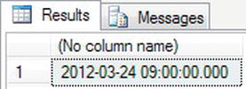
Figure 13-14. Subtracting hours from a date
DATEDIFF()
To find the difference between two dates, use the function DATEDIFF(). The syntax for this function is as follows:
DATEDIFF(datepart, startdate, enddate)
The first option contains the same options as for DATEADD(), and startdate and enddate are the two days you want to compare. A negative number shows that the enddate is before the startdate.
TRY IT OUT: DATEDIFF()
You will set two local variables to a date and time. Then by using the DATEDIFF() function, you find the difference in milliseconds. Enter the following code.
DECLARE @FirstTime datetime, @SecondTime datetime

SET @FirstTime = '24 March 2011 3:00 PM'

SET @SecondTime = '24 March 2011 3:33PM'

SELECT DATEDIFF(ms,@FirstTime,@SecondTime)
Figure 13-15 shows the results after executing this code.
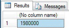
Figure 13-15. The difference between two dates in milliseconds
DATENAME()
Returning the name of the part of the date is great for using with things such as customer statements. Changing the number 6 to the word June makes for more pleasant reading.
The syntax is as follows:
DATENAME(datepart, datetoinspect)
You will also see this in action in DATEPART().
TRY IT OUT: DATENAME()
In this example, you will set one date and time and then return the day of the week. You know this to be a Thursday by checking a calendar. Enter the following code:
DECLARE @StatementDate datetime

SET @StatementDate = '24 March 2011 3:00 PM'

SELECT DATENAME(dw,@StatementDate)
Figure 13-16 shows the results after executing this code.
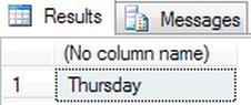
Figure 13-16. The day name of a date
DATEPART()
If you want to achieve returning part of a date from a date variable, column, or value, you can use DATEPART() within a SELECT statement.
As you may be expecting by now, the syntax has datepart as the first option, and then the datetoinspect as the second option, which returns the numerical day of the week from the date inspected.
DATEPART(datepart, datetoinspect)
TRY IT OUT: DATEPART()
- In this example, you need to set only one local variable to a date and time. After that, you find the day of the month. In this instance, the variable will have the value set at the time of the definition. Enter the following code:
DECLARE @WhatsTheDay datetime = '24 March 2013 3:00 PM'

SELECT DATEPART(dd, @WhatsTheDay)
Figure 13-17 shows the results after executing this code.
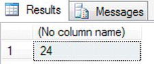
Figure 13-17. Finding part of a date
- To produce a more pleasing date and time for a statement, you can combine
DATEPART()andDATENAME()to have a meaningful output. The functionCAST(), which you will look at in detail shortly, is needed here, as it is a data type conversion function.DECLARE @WhatsTheDay datetime = '24 March 2013 3:00 PM'
SELECT DATENAME(dw, @WhatsTheDay) + ', ' +
CAST(DATEPART(dd,@WhatsTheDay) AS varchar(2)) + ' ' +
DATENAME(mm,@WhatsTheDay) + ' ' +
CAST(DATEPART(yyyy,@WhatsTheDay) AS char(4)) - When this is executed, it will produce the more meaningful date shown in Figure 13-18.
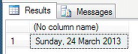
Figure 13-18. Finding and concatenating to provide a useful date
FORMAT()
The next example in this section on dates demonstrates a function that allows you to format locale-aware dates and numbers. Be aware that this function will not be available on SQL Server installations that do not have the .NET CLR installed. It does not have to be enabled. The FORMAT() function in SQL Server is similar to the function found in Excel and .NET.
TRY IT OUT: FORMAT()
- This example will return a date that is in US format and format it to display in the locale of the UK. Enter the following code:
DECLARE @MyDate DATETIME

SELECT @MyDate = 'Jun 1 2011'

SELECT FORMAT(@MyDate, 'dd MMM yyyy', 'en-GB') AS UKDate - Executing the code, you will see the date alter its format to display in the UK format, as shown in Figure 13-19.
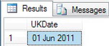
Figure 13-19. Format with a locale
DATEFROMPARTS()/SMALLDATETIMEFROMPARTS()
There may be times that you have either a date or part of a date in three variables or columns holding the year, month, and day or a combination in which one or more of these are derived and the others are supplied. It is possible to convert these three values into a valid date using DATEFROMPARTS(). You can then expand this with other functions if required.
If you want to build a time as well as a date, then you can use the SMALLDATETIMEFROMPARTS() function to achieve this.
TRY IT OUT: DATEFROMPARTS() AND SMALLDATETIMEFROMPARTS()
- This example will create five variables and define a value for each. The variable names in the example denote what each will be used for. The first
SELECTstatement will change the integers into a valid date and then format the value to show the day, the full month name, and the year. The second example appends to this the 24-hour time. Enter the first example using this code: - When you execute this code, you will see two results as shown in Figure 13-20.
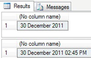
Figure 13-20. Showing dates from parts with formatting
- If you enter an invalid value—for example, setting the day to a value of 40—this will throw an error that would be the same as that here.
Msg 289, Level 16, State 1, Line 4

Cannot construct data type date, some of the arguments have values which are not valid.
TIMEFROMPARTS()
Similar to DATEFROMPARTS(), there is a TIMEFROMPARTS() function that will return a time up to fractions of a second from separate variables or values. The function takes five parameters, with the first four being hour, minute, seconds, and fractions of a second. The fifth parameter determines the precision of the fraction portion of the time. If you had a precision of 2, then the fraction number would be defined in 1/100ths.
TRY IT OUT: TIMEFROMPARTS()
- This example will create five variables and define a value for each. The variable names in the example denote what each will be used for. The precision in this example is set to 1/100ths, and therefore a value of 5 is 5/100ths.
- When you execute this code, you will see the result as shown in Figure 13-21.
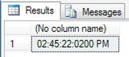
Figure 13-21. Showing times with fractions and precision from parts with formatting
DATETIME2FROMPARTS()
It is possible to combine the previous two functions to take a date and time set of values and return a datetime2 data type.
TRY IT OUT: DATETIME2FROMPARTS()
- This example will create seven variables and set a value for each. The variable names should denote what each will be used for. In this example, you will see what happens when the precision is less than the fractions of a second. A precision of zero denotes that there are no fractions to be displayed. Enter the following code.
DECLARE @Year int=2012, @Month int=6, @Day int=22

DECLARE @Hour int=23, @Minute int=45, @Seconds int=22

DECLARE @Fractions int=231


SELECT FORMAT(DATETIME2FROMPARTS(@Year,@Month,@Day,@Hour,

@Minute,@Seconds,@Fractions,0),

'hh:mm:ss:ffff tt','en-GB') - When you execute this code, an error is generated. The precision parameter defined in the function must be able to cope with the preision value presented in the fractions parameter. Truncation which you might expect in this example does not occur. The error you would see follows:
Msg 289, Level 16, State 5, Line 5

Cannot construct data type datetime2, some of the arguments have

values which are not valid. - Correct the code by altering the
@Precisionvariable to 3, and when the code is executed with the correction, you should see the output as shown in Figure 13-22.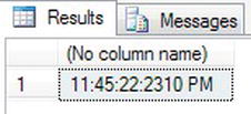
Figure 13-22. Showing
datetime2data type from date and time parts with formatting
DATETIMEOFFSETFROMPARTS()
There will be times when you have a date and a time and you have to apply an offset to it. One example would be when you are working with different time zones or you want to add to a date and time how long a response queue estimate is before a response to a query. Adding an hour and minute offset to a date and time will provide you with this functionality. The DATETIMEOFFSETFROMPARTS() function still has the ability to work in fractions and precision, keeping it in alignment with the other “from parts” functions.
TRY IT OUT: DATETIMEOFFSETFROMPARTS()
- This example will create nine variables and define a value for each. The variable names in the example denote what each will be used for. In this example, you are adding 3 hours and 12 minutes to the time. This will cause the day portion to move to the next day. Enter the following code:
DECLARE @Year int=2012, @Month int=6, @Day int=22

DECLARE @Hour int=23, @Minute int=45, @Seconds int=22

DECLARE @HourOffset int=3, @MinuteOffset int=12

DECLARE @Fractions int=0


SELECT DATETIMEOFFSETFROMPARTS(@Year,@Month,@Day,

@Hour,@Minute,@Seconds,@Fractions,@HourOffset, @MinuteOffset,0) - When you execute this code, you will see the result as shown in Figure 13-23.
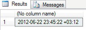
Figure 13-23. Showing a date and time moved for an offset
- You can also move the offset backward by having negative hour and minute offsets. In the following example, it is moving the date and time back in time. You could use this functionality to check date and time of delivery, represented by the values in the variables, against a date and time retrieved from variables or columns to check if you have met your target.
DECLARE @Year int=2012, @Month int=6, @Day int=22

DECLARE @Hour int=23, @Minute int=45, @Seconds int=22

DECLARE @HourOffset int=-6, @MinuteOffset int=-50

DECLARE @Fractions int=0


SELECT DATETIMEOFFSETFROMPARTS(@Year,@Month,@Day,

@Hour,@Minute,@Seconds,@Fractions,

@HourOffset, @MinuteOffset,0) - If you execute the foregoing code, you should see a result as shown in Figure 13-24.
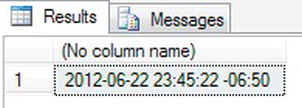
Figure 13-24. Showing time offset that is in the past
EOMONTH()
Knowing the last day of the month can be more important than knowing the first day of the month, as months vary in the number of days they have. By knowing the last day of the month, you can work backward or even add one day to get the first day of the next month. This is achieved in SQL Server using EOMONTH(), which can also have a date offset option with it.
TRY IT OUT: EOMONTH()
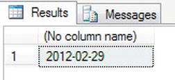
- This example will use
EOMONTH()to find the last day of February 2012. It will use January as the month and then add one month to this date, demonstrating how you can find the last date of the next month. Enter the following code.SELECT EOMONTH('Jan 12 2012',1) - When you execute this code, you will see the result as shown in Figure 13-25, showing the end of the month of February 2012 to be the 29th, as it is a leap year.
GETDATE()/SYSDATETIME()
GETDATE() is a great function for returning the exact date and time from the system. You have seen this in action when setting up a table with a default value, as well as at a couple of other points in the book. There are no parameters. If you need accuracy to nanoseconds and further, then use SYSDATETIME().
String
This next section will look at some functions that can act on character-based types, such as varchar and char.
ASCII()
ASCII() converts a single character to the equivalent ASCII code.
TRY IT OUT: ASCII()
- This example will return the ASCII code of the first character within a string. If the string has more than one character, then only the first will be taken.
DECLARE @StringTest char(10)

SET @StringTest = ASCII('Robin     ')

SELECT @StringTest - Executing the code, you will see the ASCII value of the letter “R” returned, as shown in Figure 13-26.
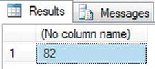
Figure 13-26. An ASCII value
CHAR()
The reverse of ASCII() is the CHAR() function, which takes a numeric value within the ASCII character range and turns it into an alphanumeric character.
TRY IT OUT: CHAR()
- In this example, you will define a local variable. Notice that the variable is a character-based data type. You then place the
ASCII()value of “R” into this variable. From there, you convert back to aCHAR(). There is an implicit conversion from a character to a numeric. If the conversion results in a value greater than 255—the last value for an ASCII character—thenNULLis returned. Enter the following code:DECLARE @StringTest char(10)
SET @StringTest = ASCII('Robin ')
SELECT CHAR(@StringTest) - Executing the code, you will see an “R,” as shown in Figure 13-27.
Figure 13-27. Changing a number to a character
- The same result would be derived using a data type that is expected that is numeric-based.
DECLARE @StringTest int

SET @StringTest = ASCII('Robin     ')

SELECT CHAR(@StringTest)
LEFT()
When it is necessary to return the first n left characters from a string-based variable, you can achieve this through the use of LEFT(), replacing n with the number of characters you want to return.
TRY IT OUT: LEFT()
- In this example, you will take the first three characters from a local variable. Here you are taking the first three characters from Robin to return Rob:
- As expected, you should get the results shown in Figure 13-28 when you execute the code.
Figure 13-28. The first
LEFTcharacters
LOWER()
To change alphabetic characters within a string, ensuring that all characters are in lowercase, you can use the LOWER() function.
TRY IT OUT: LOWER()
- The
LOWER()example will combine this function along with another string function,LEFT(). Like all the functions, they can be combined together to perform several functions all at once.DECLARE @StringTest char(10)
SET @StringTest = 'Robin '
SELECT LOWER(LEFT(@StringTest,3)) - As you can see, this results in displaying rob in lowercase, as shown in Figure 13-29.
Figure 13-29. Changing letters to lowercase
LTRIM()
There will be times that leading spaces will occur in a string that you’ll want to remove. LTRIM() will trim these spaces on the left.
TRY IT OUT: LTRIM()
- To prove that leading spaces are removed by the
LTRIM()function, you have to change the value within the local variable. On top of that, you have to put a string prefixing the variable to show that the variable has had the spaces removed.DECLARE @StringTest char(10)
SET @StringTest = ' Robin'
SELECT 'Start-'+LTRIM(@StringTest),'Start-'+@StringTest - You produce two columns of output, as shown in Figure 13-30: the first with the variable trimmed and the second showing that the variable did have the leading spaces.
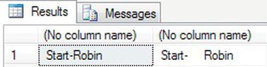
Figure 13-30. Removing spaces from the left
RIGHT()
The opposite of LEFT() is, of course, RIGHT(), and this function returns the characters from the right-hand side.
TRY IT OUT: RIGHT()
- Keep the variable used in
LTRIM(), as it will allow you to returnbin, which are the three characters on the right-hand side of the variable.DECLARE @StringTest char(10)
SET @StringTest = ' Robin'
SELECT RIGHT(@StringTest,3) - The results should appear as shown in Figure 13-31.
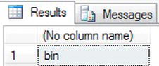
Figure 13-31. Returning a number of characters starting from the right
RTRIM()
When you have a CHAR() data type, no matter how many characters you enter, the variable will be filled on the right, known as right-padded, with spaces. To remove these, use RTRIM. This changes the data from a fixed-length CHAR() to a variable-length value.
TRY IT OUT: RTRIM()
- This example has no spaces after Robin, and you will remove the space padding within the first column returned from the following code. The second column has the spaces trimmed.
DECLARE @StringTest char(10)

SET @StringTest = 'Robin'

SELECT @StringTest+'-End',RTRIM(@StringTest)+'-End' - The results are as expected, as shown in Figure 13-32.
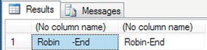
Figure 13-32. Removing spaces from the right
STR()/CONCAT()
Some data types have implicit conversions. You will see later how to do explicit conversions, but a simple conversion that will take any numeric value and convert it to a variable-length string is STR(), which you will look at next. However, SQL Server sometimes has to decide which way the conversion has to go. You will see this problem in the first example in the “Try It Out” exercise. If you want to concatenate two values into a string, then, as you will see in the second example, you will invoke the STR() function. However, you will see that this also causes a little bit more work to be done within the code to achieve the desired results. To concatenate two values, you can use the CONCAT() function, similar to the function found in Excel.
TRY IT OUT: STR()
- The first example demonstrates that you cannot add a number, 82, to a string.
SELECT 'A'+82 - When the preceding code is executed, you will see the following error:
- Changing the example to include the
STR()function will convert this numeric to a string of varying length, such asvarchar().SELECT 'A'+STR(82) - Instead of an error, you now see the desired result, which appears in Figure 13-33. However, it isn’t really desirable as there are spaces between the letter and the number. Leading zeros are translated to spaces.
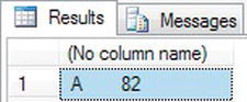
Figure 13-33. Changing a number to a string
- By including an
LTRIM()invocation, you can remove those spaces.SELECT 'A'+LTRIM(STR(82)) - This code now produces the correct results, as you see in Figure 13-34.
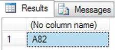
Figure 13-34. Changing a number to a string and removing leading spaces
- A cleaner set of code that removes the need for
LTRIMandSTRfunctions would be to use theCONCATfunction. The code here demonstrates how simple the code can be.SELECT CONCAT('A',82) - This will produce the results in Figure 13-35.
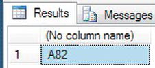
Figure 13-35. Using
CONCATto concatenate mixed data types
SUBSTRING()
As you have seen, you can take a number of characters from the left and from the right of a string. To retrieve a number of characters that do not start with the first or last character, you need to use the function SUBSTRING(). This has three parameters: the variable or column, which character to start the retrieval from, and the number of characters to return.
TRY IT OUT: SUBSTRING()
- Define the variable you want to return a substring from. Once complete, you can then take the variable, inform SQL Server you want to start the substring at character position 3, and return the next 2 characters.
DECLARE @StringTest char(10)

SET @StringTest = 'Robin     '

SELECT SUBSTRING(@StringTest,3,2) - And you have the desired result, as shown in Figure 13-36.
Figure 13-36. Returning part of a string from within a string
UPPER()
The final string example is the reverse of the LOWER() function and changes all characters to uppercase.
TRY IT OUT: UPPER()
- After the declared variable has been set, you then use the
UPPER()function to change the value to uppercase.DECLARE @StringTest char(10)
SET @StringTest = 'Robin '
SELECT UPPER(@StringTest) - Execute the foregoing code and, as you can see from Figure 13-37, Robin becomes ROBIN.
System Functions
System functions are functions that provide extra functionality outside of the boundaries that can be defined as string-, numeric-, or date-related. Three of these functions will be used extensively throughout your code, and therefore you should pay special attention to CASE, CAST, and ISNULL.
CASE WHEN...THEN...ELSE...END
The first function is for when you want to test a condition. WHEN that condition is true, THEN you can do further processing; ELSE if it is false, then you can do something else. What happens in the WHEN section and the THEN section can range from another CASE statement to providing a value that sets a column or a variable.
The CASE WHEN statement can be used to return a value or, if on the right-hand side of an equality statement, to set a value. Both of these scenarios are covered in the following examples.
TRY IT OUT: CASE
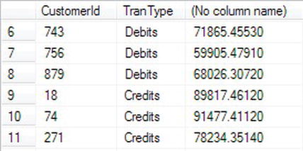
- The example will use a
CASEstatement to add up customers’TransactionDetails.Transactionsfor the month of August. If theTransactionTypeis 0, then this is a Debit; if it is a 1, then it is a Credit. By using theSUMaggregation, you can add up the amounts. Combine this with aGROUP BYwhere theTransactionDetails.Transactionsare split between Credit and Debit, and you get two rows in the results set: one for debits and one for credits.SELECT CustomerId,
CASE WHEN CreditType = 0 THEN 'Debits' ELSE 'Credits' END
AS TranType,SUM(Amount)
FROM TransactionDetails.Transactions t
JOIN TransactionDetails.TransactionTypes tt ON
tt.TransactionTypeId = t.TransactionType
WHERE t.DateEntered BETWEEN '1 Jan 2012' AND '4 Jan 2012'
GROUP BY CustomerId,CreditType - When the code is run, you should see the results that are partly shown in Figure 13-38.
IIF()
If you have used Excel or Access among some other tools, you have quite possibly met IIF() when coding. IIF(), also known as an inline IF, is very similar to the CASE statement demonstrated in the previous example. Where CASE can have many choices, IIF() has only two choices. The syntax is as follows:
IIF(boolean_test_condition, true_value, false_value)
TRY IT OUT: IIF()
- To demonstrate the similarity but also the reduction in the amount you have to code, I will take the example from the
CASEstatement and alter that to become anIIF()statement.SELECT CustomerId,
IIF(CreditType = 0,'Debits','Credits') 'Debit/Credit',SUM(Amount)
FROM TransactionDetails.Transactions t
JOIN TransactionDetails.TransactionTypes tt ON
tt.TransactionTypeId = t.TransactionType
WHERE t.DateEntered BETWEEN '1 Jan 2012' AND '4 Jan 2012'
GROUP BY CustomerId,CreditType - Figure 13-39 will have similar output as Figure 13-39; the alias for the
Debit/Creditcolumn has been altered to show that a different set of code has run.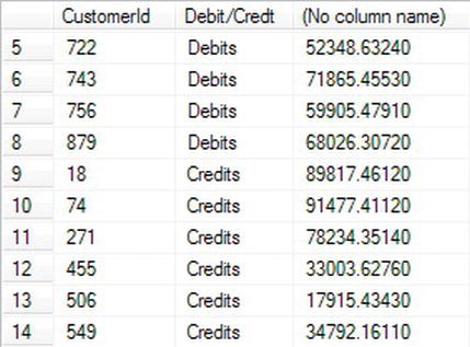
CHOOSE()
The ability to return a value based on a separate value can be useful. A good explanation example would be a number that has a range of one through seven could be used as the basis of determining the day name of the week. There is a function that already does this, as demonstrated earlier in the chapter with DATENAME(). In the ApressFinancial database, it might have been possible to use CHOOSE() for the transaction types to denote a debit or a credit type. However, for only two choices, IIF() is a better option. CHOOSE() is good for where there are three or more possible options for the testing value and translating it to a new value.
There is a large caveat, and that is that you should not necessarily replace tables that have a few rows with a CHOOSE() statement. Having the data in a table gives a number of advantages, including a single point for the data and the ability to join the data; if you have to add any new data, you can simply add it to the table rather than having to alter one or more stored procedures and functions.
I am yet to be convinced of using CHOOSE() instead of a cross-reference table unless you have the CHOOSE() choices within a user-defined function. So, for example, you would place the following example as a user-defined function to return the choice value rather than the TransactionDetails.TransactionTypes table.
TRY IT OUT: CHOOSE()
- This example demonstrates how you could move the
TransactionDetails.TransactionTypestable functionality into aCHOOSE()statement. Although this works and demonstrates theCHOOSE()statement, it should also demonstrate that it is not always appropriate to take data from a table and replace the logic and functionality that having data in a table provides. - When you execute the code, you will see the results shown in Figure 13-40.
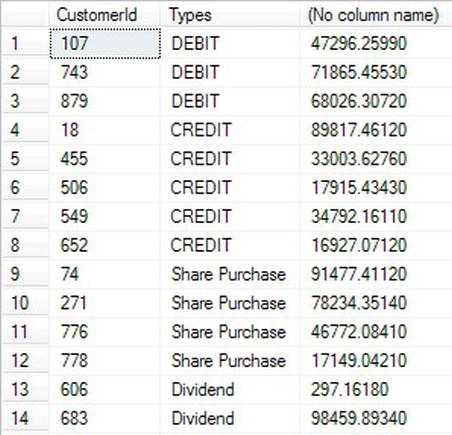
Figure 13-40.
CHOOSEreturning transaction types instead of a table
CAST()/CONVERT()
These are two functions used to convert from one data type to another. The main difference between them is that CAST() is ANSI SQL–92 compliant, but CONVERT() has more functionality.
The syntax for CAST() is as follows:
CAST(variable_or_column AS datatype)
This is opposed to the syntax for CONVERT(), which is as follows:
CONVERT(datatype,variable_or_column)
Not all data types can be converted between each other, such as converting a datetime to a text data type, and some conversions need neither a CAST() nor a CONVERT(). There is a grid in “Books Online” that provides the necessary information.
If you want to CAST() from numeric to decimal or vice versa, you need to use CAST(); otherwise, you will lose precision.
TRY IT OUT: CAST()/CONVERT()
- The first example will use
CASTto move a number to achar(10).DECLARE @Cast int
SET @Cast = 1234
SELECT CAST(@Cast as char(10)) + '-End' - Executing this code results in a left-filled character variable, as shown in Figure 13-41.
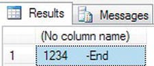
Figure 13-41. Changing the data type of a value
- The second example completes the same conversion, but this time you use the
CONVERT()function.DECLARE @Convert int
SET @Convert = 5678
SELECT CONVERT(char(10),@Convert) + '-End' - As you can see from Figure 13-42, the only change is the value output.
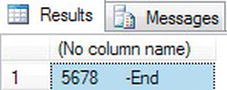
Figure 13-42. Changing the data type of a value, using the non-ANSI standard
ISDATE()
Although ISDATE() is a function that works with dates and times, this system function takes a value in a column or a variable and confirms whether it contains a valid date or time. The value returned is 0, or false, for an invalid date, or 1 for true if the date is okay. The formatting of the date for testing within the ISDATE() function has to be in the same regional format as you have set with SET DATEFORMAT or SET LANGUAGE. If you are testing in a European format but have your database set to US format, then you will get a false value returned.
TRY IT OUT: ISDATE()
- The first example demonstrates where a date is invalid. There are only 30 days in September.
DECLARE @IsDate char(15)

SET @IsDate = '31 Sep 2011'

SELECT ISDATE(@IsDate) - Execute the code, and you should get the results shown in Figure 13-43.
Figure 13-43. Testing if a value is a valid date and showing it is invalid
- The second example is a valid date.
DECLARE @IsDate char(15)

SET @IsDate = '30 Sep 2011'

SELECT ISDATE(@IsDate) - This time when you run the code, you see a value of 1, as shown in Figure 13-44, denoting a valid entry.
Figure 13-44. Showing that a value is a valid date
- You can then combine this with a
CASEstatement to test whether a variable is a valid date; if it is, you can then format the date as you wish or display something if the date is invalid. In the following exercise, achar()data type is tested as to whether it is a date. If it is, it is then converted from achar()to adatedata type and then formatted.DECLARE @IsDate char(15)
SET @IsDate = '30 Sep 2011'
SELECT CASE WHEN ISDATE(@IsDate) = 1
THEN FORMAT(CONVERT(DATE,@IsDate),'MMM dd yyyy', 'en-GB')
ELSE 'Invalid Date'
END AS 'DateOutput' - The code checks if the value is a date. When it is, the value will be converted and formatted. You should see the date in the month, day, year format, as shown in Figure 13-45.
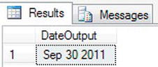
Figure 13-45. Checking if the value is a valid date and formatting it
ISNULL()
Many times so far, you have seen NULL values within a column of returned data. As a value, NULL is very useful, as you have seen. However, you may want to test whether a column contains a NULL. If there were a value, you would retain it, but if there were a NULL, you would convert it to a value. This function could be used to cover a NULL value in an aggregation, for example. The syntax is as follows, where the first parameter is the column or variable to test if there is a NULL value, and the second option defines what to change the value to if there is a NULL value:
ISNULL(value_to_test,new_value)
This change occurs only in the results and doesn’t change the underlying data that the value came from.
TRY IT OUT: ISNULL()
- In this example, you define a
char()variable of ten characters in length and then set the value explicitly toNULL. The example will also work without the second line of code, which is simply there for clarity. The third line tests the variable, and as it isNULL, it changes it to a date. Note, though, that a date is more than ten characters, so the value is truncated.DECLARE @IsNull char(10)
SET @IsNull = NULL
SELECT ISNULL(@IsNull,GETDATE()) - As expected, when you execute the code, you get the first ten characters of the relevant date, as shown in Figure 13-46.
Figure 13-46. Changing a
NULLvalue to a different value in the results
ISNUMERIC()
This system function tests the value within a column or variable and ascertains whether it is numeric. The value returned is 0, or false, for an invalid number, or 1 for true if the value can be converted to a numeric.
![]() Note Currency symbols such as £ and $ will also return
Note Currency symbols such as £ and $ will also return 1 for a valid numeric value.
TRY IT OUT: ISNUMERIC()
- The first example to demonstrate
ISNUMERIC()defines a character variable and contains alphabetic values. This test fails, as shown in Figure 13-47.DECLARE @IsNum char(10)
SET @IsNum = 'Robin '
SELECT ISNUMERIC(@IsNum)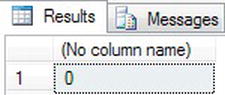
Figure 13-47. Checking whether a value is a number and finding out it is not
- This second example places numbers and spaces into a
charfield. TheISNUMERIC()test ignores the spaces, provided that there are no further alphanumeric characters.DECLARE @IsNum char(10)
SET @IsNum = '1234 '
SELECT ISNUMERIC(@IsNum) - Figure 13-48 shows the results of running this code.
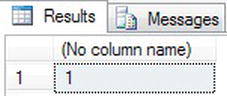
Figure 13-48. Finding out a value is numeric
TRY_CONVERT()
As you have seen in the last few examples, you can test if data fit certain data types and that you can cast from one data type to another. However, it is possible to be in a situation where you cannot cast the data to the relevant data type. In the previous example, an error would be received if you tried to convert to a data type where the data were not valid. Using TRY…CONVERT(), you can attempt to cast the data, and if the conversion is not possible, a NULL value is returned.
One example of where TRY…CONVERT() would be better than a straight conversion is where data that are valid in one system are transferred and not valid in another. An example of this is where one system for a date can hold a specific date, a date range, or a date length such as three months. Another example is where mnemonics are stored for a number, like M for million. The receiving system could then use the TRY_CONVERT() to place the data in one of three columns depending on the scenario. By using TRY…CONVERT() and the CASE statement, you could fulfill the three tests on the date and populate the relevant correct column in your system. The example you will see demonstrated will show this.
TRY IT OUT: TRY_CONVERT()
- The first example will try to convert “3 months” to a date. This will fail and therefore return a
NULLvalue.DECLARE @InputDate char(15)
SET @InputDate = '3 Months'
SELECT TRY_CONVERT(DATE,@InputDate) AS OutputDate - Executing this code results in a
NULLvalue as this is not a valid date, as shown in Figure 13-49.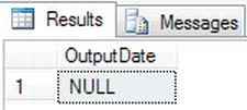
Figure 13-49. Trying to convert an invalid date to a date
- It is possible to extend the code so that it attempts to convert the data to a valid data type, and if it is unable to convert, to use a default data value. The code here shows one method of combining
IIF()withTRY_CONVERT. I have placed the three different settings that can be used to test the code.DECLARE @InputDate char(15), @DateValue date, @DateRange date
DECLARE @Default varchar(15)
-- SET @InputDate = '3 Sep 2011'
-- SET @InputDate = '
0
3'
SET @InputDate = 'Rubbish'
SELECT @DateValue = TRY_CONVERT(DATE,@InputDate),
@DateRange = IIF(TRY_CONVERT(int,@InputDate) IS NULL,NULL,
DATEADD(d,CONVERT(int,@InputDate),'30 Dec 2012')),
@Default = IIF(TRY_CONVERT(DATE,@InputDate) IS NULL,
IIF(TRY_CONVERT(int,@InputDate) IS NULL,@InputDate,
NULL),NULL)
SELECT @DateValue, @DateRange, @Default - Executing the three different tests will give the results shown in Figure 13-50.
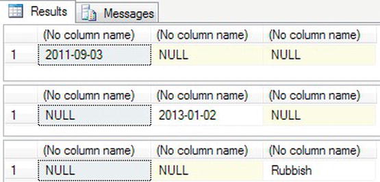
Figure 13-50. Three test results for each
TRY_CONVERTtest
PARSE/TRY_PARSE()
CAST and CONVERT are ideal for general conversion, but for specific conversions from string to a number or a datetime, then PARSE is the preferred option. From other data types, you should use CONVERT/TRY_CONVERT. PARSE is similar to CONVERT, and, as you might expect, TRY_PARSE is similar to TRY_CONVERT, in that you can test the variable, and if the cast fails, then a NULL value is returned. It is possible to include culture information as part of the parsing so that the conversion takes the defined locale into consideration.
TRY IT OUT: PARSE() AND TRY_PARSE()
- The first example will try to parse “KJ” to an integer. This will fail and return an error, as it assumes that the incoming value is of a valid data type.
DECLARE @InputNumber char(2)

SET @InputNumber = 'KJ'

SELECT PARSE(@InputNumber as int) AS OutputNumeric - Execute the code and you should see the following:
- The next example will try to parse “KJ” to an integer, which would be the better solution if there is a chance the data type is involved. This will fail but this time will return a
NULLvalue.DECLARE @InputNumber char(2)
SET @InputNumber = 'KJ'
SELECT TRY_PARSE(@InputNumber as int) AS OutputNumeric - Execute the code, and you should see a better result, as shown in Figure 13-51.
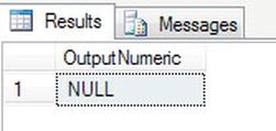
Figure 13-51. Trying to parse a string variable to a number
Even though the many system functions, several of which allow you to test data to try to avoid an unexpected error occurring, have been demonstrated, you can never plan for every eventuality. In the following section, you will see how to work with errors when they do occur.
RAISERROR
Before you learn about handling errors, you need to be aware of what an error is, how it is generated, the information it generates, and how to generate your own errors when something is wrong. The T-SQL command RAISERROR allows you as a developer to have the ability to produce your own SQL Server error messages when running queries or stored procedures. You are not tied to using just error messages that come with SQL Server; you can set up your own messages and your own level of severity for those messages. It is also possible to determine whether the message is recorded in the Windows error log.
However, whether you want to use your own error message or a system error message, you can still generate an error message from SQL Server as if SQL Server itself raised it. Enterprise environments typically experience the same errors on repeated occasions, since they employ SQL Server in very specific ways depending on their business model. With this in mind, attention to employing RAISERROR can have big benefits by providing more meaningful feedback as well as suggested solutions for users. You will see later in the chapter a second method for generating an error.
By using RAISERROR, SQL Server acts as if SQL Server raised the error, as you have seen within this book.
RAISERROR can be used in one of two ways; looking at the syntax will make this clear.
You can either use a specific msg_id or provide an actual output string, msg_str, either as a literal or a local variable defined as string-based, containing the error message that will be recorded. The msg_id references system and user-defined messages that already exist within the SQL Server error messages table.
When specifying a text message in the first parameter of the RAISERROR function instead of a message ID, you may find that this is easier to write than creating a new message:
RAISERROR('You made an error', 10, 1)
The next two parameters in the RAISERROR syntax are numerical and relate to how severe the error is and information about how the error was invoked. Severity levels range from 1 at the innocuous end to 25 at the fatal end. Severity levels of 2 to 14 are generally informational. Severity level 15 is for warnings, and levels 16 or higher represent errors. Severity levels from 20 to 25 are considered fatal, and require the WITH LOG option, which means that the error is logged in the Windows Application Event Log and the SQL error log and the connection terminated; quite simply, the stored procedure stops executing. The connection referred to here is the connection within Query Editor, or the connection made by an application using a data access method like ADO.NET. Only for a most extreme error would you set the severity to this level; in most cases, you would use a number between 1 and 19.
The last parameter of the function specifies state. Use a 1 here for most implementations, although the legitimate range is from 1 to 127. You may use this to indicate which error was thrown by providing a different state for each RAISERROR invocation in your stored procedure. SQL Server does not act on any legitimate state value, but the parameter is required.
A msg_str can define parameters within the text. By placing the value, either statically or via a variable, after the last parameter that you define, msg_str replaces the message parameter with that value. This is demonstrated in an upcoming example. If you do want to add a parameter to a message string, you have to define a conversion specification. The format is as follows:
% [[flag] [width] [. precision] [{h | l}]] type
The options are as follows:
flag: A code that determines justification and spacing of the value entered:-
-(minus): Left-justify the value
-
+(plus): The value shows a + or a–sign.-
0: Prefix the output with zeros
-
#: Preface any nonzero with a 0, 0x, or0X, depending on the formatting- (blank): Prefix with blanks
width: The minimum width of the outputprecision: The maximum number of characters used from the argumenth: Character types:- To place a parameter within a message string where the parameter needs to be inserted, put a
%sign followed by one of the following options:dorifor a signed integer,pfor a pointer,sfor a string,ufor an unsigned integer,xorXfor an unsigned hexadecimal, andofor an unsigned octal. Note that float, double, and single are not supported as parameter types for messages. You will see this in the upcoming examples.
Finally, there are three options that could be placed at the end of the RAISERROR message. These are the WITH options:
LOGplaces the error message within the Windows error log.NOWAITsends the error directly to the client.SETERRORresets the error number to 50000 within the message string only.
When using any of these last WITH options, do take the greatest of care, as their misuse can create more problems than they solve. For example, you may unnecessarily use LOG a great deal, filling up the Windows Application Event Log and the SQL error log, which leads to further problems.
There is a system stored procedure, sp_addmessage, that can create a new global error message that can be used by RAISERROR by defining the @msgnum. The syntax for adding a message is as follows:
sp_addmessage [@msgnum =]msg_id,

[@severity = ] severity , [ @msgtext = ] 'msg'

     [ , [ @lang = ] 'language' ]

     [ , [ @with_log = ] 'with_log' ]

     [ , [ @replace = ] 'replace' ]
The parameters into this system stored procedure are as follows:
@msgnum: The number of the message is typically greater than 50000.@severity: A number in the range of 1 to 25@lang: Use this if you need to define the language of the error message. Normally, this is left empty.@with_log: Set to'TRUE'if you want to write a message to the Windows error log.@replace: Set to'replace'if you are replacing an existing message and updating any of the preceding values with new settings.
![]() Note Any message added will be specific for that database rather than the server.
Note Any message added will be specific for that database rather than the server.
It is time to move to an example that will set up an error message that will be used to say a customer is overdrawn.
TRY IT OUT: RAISERROR
Error Handling
When working with T-SQL, it is important to have some sort of error handling to cater to those times when something goes wrong. Errors can be of different varieties; for example, you might expect at least one row of data to be returned from a query, and then you receive no rows. However, what I am discussing here is when SQL Server informs you there is something more drastically wrong. You have seen some errors throughout the book, and even in this chapter. There are two methods of error catching you can employ in such cases. The first uses a system variable, @@ERROR.
@@ERROR
This is the most basic of error handling. It has served SQL Server developers well over the years, but it can be cumbersome. When an error occurs, such as you have seen as you have gone through the book creating and manipulating objects, a global variable, @@ERROR, is set with the SQL Server error message number. Similarly, if you try to do something with a set of data that is invalid, such as dividing a number by zero or exceeding the number of digits allowed in a numeric data type, then SQL Server will set this variable for you to inspect.
The downside is that the @@ERROR variable setting lasts only for the next statement following the line of code that has been executed; therefore, when you think there might be problems, you need to either pass the data to a local variable or inspect it straightaway. The first example demonstrates this.
TRY IT OUT: USING @@ERROR
- This example tries to divide 100 by zero, which is an error. You then list out the error number, and then again list out the error number. Enter the following code and execute it:
SELECT 100/0

SELECT @@ERROR

SELECT @@ERROR - It is necessary in this instance to check both the Results and Messages tabs. The first tab is the Messages tab, which shows you the error encountered. As expected, you see the “Divide by zero error encountered” message.
Msg 8134, Level 16, State 1, Line 1

Divide by zero error encountered.

(1 row(s) affected)

(1 row(s) affected)
- Moving to the Results tab, you should see three result sets, as shown in Figure 13-52. The first, showing no information, would be where SQL Server would have put the division results, had it succeeded. The second result set is the number from the first
SELECT @@ERROR. Notice the number corresponds to themsgnumber found in the Messages tab. The third result set shows a value of0. This is because the firstSELECT @@ERRORworked successfully and therefore set the system variable to0. This demonstrates the lifetime of the value within@@ERROR.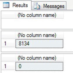
Figure 13-52. Showing
@@ERRORin multiple statements - When you use the
RAISERRORfunction, it also sets the@@ERRORvariable, as you can see in the following code. However, the value will be set to0using the preceding example. This is because the severity level was below 11.RAISERROR (50001,1,1,243)
SELECT @@ERROR - When the code is executed, you can see that
@@ERRORis set to0, as shown in Figure 13-53.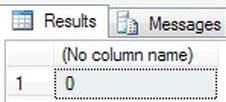
Figure 13-53. When severity is too low to set
@@ERROR - By changing the severity to 11 or above, the
@@ERRORsetting will now be set to the message number within theRAISERROR.RAISERROR (50001,11,1,243)
SELECT @@ERROR - The preceding code produces the same message as shown within the
RAISERRORexample, but as you can see in Figure 13-54, the error number setting now reflects that value placed in themsgnumparameter.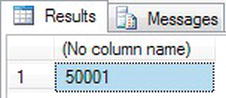
Figure 13-54. With a higher severity, the message number is set.
Although a @@ERROR is a useful tool, it would be better to use the next error-handling routine to be demonstrated, TRY...CATCH with THROW.
TRY...CATCH and THROW
It can be said that no matter what, any piece of code has the ability to fail and generate some sort of error. For the vast majority of this code, you will want to trap any error that occurs, check what the error is, and deal with it as best you can. As you saw previously, this could be done one statement at a time using @@ERROR to test for any error code. Improved functionality exists whereby a set of statements can try to execute, and if any statement has a runtime error, it will be caught. This is known as a TRY...CATCH block. If you find an error within your code where you were expecting something such as a specific value or a range of values, for example, then it is possible to generate an errorwith a THROW statement. In essence, TRY…CATCH and THROW are greatly improved and more flexible versions of RAISERROR and @@ERROR. There is one slight catch, and that is a THROW statement must be preceded with a line of code that is terminated with a semicolon.
Surrounding a single batch of code with the ability to execute that code and to then catch any errors and try to deal with them has been around for quite a number of years in languages such as C++. Gladly, you see this within SQL Server. You can use TRY…CATCH with a transaction; however, you have to take care where to place the BEGIN TRANSACTION along with the ROLLBACK and COMMIT TRANSACTION statements. You will see an example of this within the examples.
The syntax for TRY...CATCH is pretty straightforward. There are two “blocks” of code. The first block, BEGIN TRY, is where there is one or more T-SQL statements that you want to try to run. If any of statements has an error, then no further processing within that block will be done, and processing will switch to the second block, BEGIN CATCH.
BEGIN TRY

     { sql_statement | statement_block }

END TRY

BEGIN CATCH

     { sql_statement | statement_block }

END CATCH
It is possible to generate your own error via a RAISERROR, as you saw earlier, or you can execute a THROW statement either within or outside a TRY or CATCH block. A RAISERROR within a TRY…CATCH will work as it would outside a TRY...CATCH, and that is that it will set the error details, and then if the severity is 10 or lower, processing will continue. If the severity is in the range of 11 to 19, then the RAISERROR would pass execution to the CATCH block. Any severity of 20 or above would stop execution immediately and close the connection, and processing would not pass to the CATCH block. Rather than using RAISERROR, you can THROW an error that will always move the execution of the code to the CATCH block of code. This allows you as a developer to do cleanup actions when an error has occurred, such as to roll back a transaction or do any other actions that you want to perform that will help you with any investigation.
TRY…CATCH blocks can be nested. This gives you several advantages. The first is that you can pass any error up through the nested levels with a rethrow. This is achieved by issuing the THROW statement with no parameters in each CATCH block in the nesting. You will sometimes hear this called “bubbling up the error.” There are advantages to bubbling as it allows a controlled way of getting out of a difficult situation; however, it can also lead to confusion if you rethrow every exception. So when you rethrow an error, ensure that this is the action you want to do.
Nesting allows you to surround a stored procedure call with a TRY…CATCH. This will then allow for any error in the called stored procedure that is thrown to be caught in the calling stored procedure.
Within the TRY…CATCH block, it is possible to retrieve error information. The system functions that can be used to find useful debugging information are detailed here:
ERROR_LINE(): The line number that caused the error or performed theRAISERRORor theTHROWstatement; this is physical rather than relative (i.e., you don’t have to remove blank lines within the T-SQL to get the correct line number, unlike some software that does require this).ERROR_MESSAGE(): The text messageERROR_NUMBER(): The number associated with the messageERROR_PROCEDURE(): If you are retrieving this within a stored procedure or trigger, the name of it will be contained here. If you are running ad hoc T-SQL code, then the value will beNULL.ERROR_SEVERITY(): The numeric severity value for the errorERROR_STATE(): The numeric state value for the error
Not all errors are caught within a TRY...CATCH block, unfortunately. These are compile errors or errors that occur when deferred name resolution takes place and the name created doesn’t exist. To clarify these two points, when T-SQL code is either ad hoc or within a stored procedure, SQL Server compiles the code, looking for syntax errors. However, not all code can be fully compiled and is not compiled until the statement is about to be executed. If there is an error, then this will terminate the batch immediately. The second error that will not be caught is that if you have code that references a temporary table, for example, then the table won’t exist at runtime and column names won’t be able to be checked. This is known as deferred name resolution, and if you try to use a column that doesn’t exist, then this will also generate an error, terminating the batch.
There is a great deal more to TRY...CATCH blocks in areas that are quite advanced, but now that you know the basics, let’s look at some examples demonstrating what I have just discussed.
TRY IT OUT: TRY...CATCH…THROW
- Your first example is a simple error where you have defined an integer local variable. Within your error-handling block, after outputting a statement to demonstrate that you are within that block, you try to set a string to the variable. This is a standard error and immediately moves the execution to the
CATCHblock; the lastSELECTis not executed.DECLARE @Probs int
BEGIN TRY
SELECT 'This will work'
SELECT @Probs='Not Right'
SELECT 10+5,
'This will also work, however the error means it will not run'
END TRY
BEGIN CATCH
SELECT 'An error has occurred at line ' +
LTRIM(STR(ERROR_LINE())) +
' with error ' + LTRIM(STR(ERROR_NUMBER())) + ' ' + ERROR_MESSAGE()
END CATCH - When you run the code, you will see the first statement and then the
SELECTstatement that executes when the error is caught. You use the system functions to display relevant information, which appears in Figure 13-55.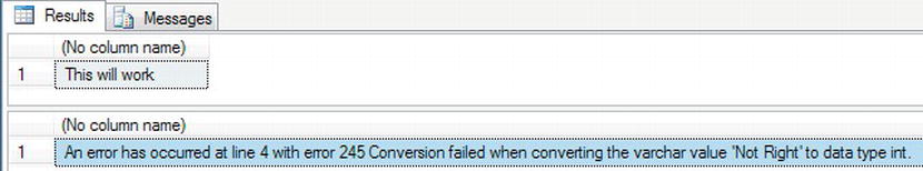
Figure 13-55. An error is caught.
- The second example demonstrates nesting
TRY...CATCHblocks and how execution can continue within the outer block when an error arises within the second block. Keep the same error and see the error message, the second catch block. But once this is executed, processing continues, and then this will now work.DECLARE @Probs int
BEGIN TRY
SELECT 'This will work'
BEGIN TRY
SELECT @Probs='Not Right'
SELECT 10+5,
'This will also work, however the error means it will not run'
END TRY
BEGIN CATCH
SELECT 'The second catch block'
END CATCH
SELECT 'And then this will now work'
END TRY
BEGIN CATCH
SELECT 'An error has occurred at line ' +
LTRIM(STR(ERROR_LINE())) +
' with error ' + LTRIM(STR(ERROR_NUMBER())) + ' ' + ERROR_MESSAGE()
END CATCH - As expected, you see three lines of output, as shown in Figure 13-56. The code in the outer
CATCHblock doesn’t run, as the error is catered to within the inner block.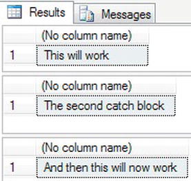
Figure 13-56. An error is caught in a nested batch.
- The foregoing example could be modified so that in the inner
CATCHblock the error is thrown to the outer catch block. The outer catch block would then hold all the rollback processing, error logging, and so on.DECLARE @Probs int
BEGIN TRY
SELECT 'This will work'
BEGIN TRY
SELECT @Probs='Not Right'
SELECT 10+5,
'This will also work, however the error means it will not run'
END TRY
BEGIN CATCH
THROW
END CATCH
SELECT 'The THROW means this is skipped'
END TRY
BEGIN CATCH
SELECT 'An error has occurred at line ' +
LTRIM(STR(ERROR_LINE())) +
' with error ' + LTRIM(STR(ERROR_NUMBER())) + ' ' + ERROR_MESSAGE()
IF @@TRANCOUNT > 0
ROLLBACK TRAN
END CATCH - After you execute the foregoing code and the error occurs, control will be passed to the inner catch block, which will then
THROWthe error to the next nesting level. In this example, control is passed to the outer block of code where the error is listed. A test is then performed to roll back any open transactions as part of the cleanup exercise. You can see the output in Figure 13-57.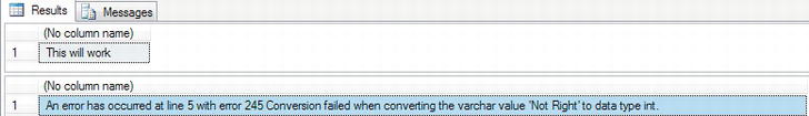
- This time, you see how your T-SQL code can be successfully precompiled and execution started. Then when you try to display results from a temporary table that doesn’t exist, the
CATCHblock does not fire, as execution terminates immediately.DECLARE @Probs int
BEGIN TRY
SELECT 'This will work'
BEGIN TRY
SELECT * FROM #Temp
END TRY
BEGIN CATCH
SELECT 'The second catch block'
END CATCH
SELECT 'And then this will now work'
END TRY
BEGIN CATCH
SELECT 'An error has occurred at line ' +
LTRIM(STR(ERROR_LINE())) +
' with error ' + LTRIM(STR(ERROR_NUMBER())) + ' ' + ERROR_MESSAGE()
END CATCH - When the code is run in the Messages tab, you see the following output, detailing one row has been returned, which comes from the first
SELECTstatement. You then see the SQL Server error. Looking at Figure 13-58, you also see just the firstSELECTstatement output.
(1 row(s) affected)

Msg 208, Level 16, State 0, Line 5

Invalid object name '#Temp'.
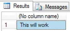
Figure 13-58. What happens when SQL Server terminates execution
- The next example demonstrates how to throw an error in an inner exception handler to an outer handler. You would normally see this in nested stored procedures, but for simplicity it will be demonstrated in the following simplified example.
BEGIN TRY
   SELECT 'Outer level'

   BEGIN TRY

      SELECT 'Inner level';

      THROW 51200, 'Inner level throw', 1

   END TRY

   BEGIN CATCH

      SELECT 'Inner Catch with re-throw';

      THROW

   END CATCH

END TRY

BEGIN CATCH

   SELECT 'Outer Catch';

   THROW

END CATCH
Note Remember that the previous statement to a THROWmust be terminated by a semicolon. - The inner throw will be passed to the inner catch, which will rethrow the error to the outer catch, which in turn throws the error to the outermost calling code, which in this instance is the end of the code, which finally lists the error. You can see this tracked in the output from the foregoing executed code in the results in Figure 13-59.
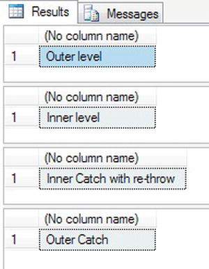
Figure 13-59. What happens when SQL Server terminates execution
- The error itself is placed in the Messages tab, which is shown here.
Error handling and having the ability to control errors will lead to code that is more robust, and when an error occurs it can be tracked in a more constructive fashion as well as handled in a controlled manner. Remembering to use a semicolon in the statement prior to a THROW may seem odd; however, this is Microsoft trying to take you down the route of statement termination via a delimiter.
Summary
The text for this chapter is not the most fluid, but the information will be very useful as you start using SQL Server. Each section you have read contains a great deal of useful and pertinent information, and rereading the chapter and maybe even trying out different ideas based on the basics demonstrated will give you a stronger understanding of what is happening. The main areas of focus were error handling and joining tables to return results. Also looking at some of the system predefined functions and how useful they can be is important, as you will use some of these functions a great number of times when coding. Take time to fully understand what is happening and how you can use these two features.