C H A P T E R 10
Selecting and Updating Data
In this chapter, you will see details on how to retrieve data correctly and professionally in a production environment, and this chapter will lay the foundation for more advanced T-SQL in the forthcoming chapters. Up until now, you have witnessed a “lazy” method in that you have returned data from every column and every row in whatever tables you have been querying. This chapter will detail why that is not ideal, and it will demonstrate the correct methods. You will also see how to change column headings so that they provide more meaningful names for non-IT people. Then you will see how to reduce the data brought back by filtering for only the rows you want. The final sections in this chapter on retrieving data will introduce you to some basic string functions, how to order the data, and how to find data when you are not quite sure of all the information.
It is also possible to create a table by selecting data from another table. You'll learn how to do that too. Creating one table from another is ideal if you need to keep a temporary copy of certain data.
As I have mentioned many times throughout the book, securing your data is just as crucial, if not more so, than the design and creation of your database. You will see how to tighten up security so that a user can select data from only one specific table.
You will then move on to updating and deleting your data. You will see how transactions are involved in both of these processes, and you'll learn how to delete an entire table of data quickly, without using the traditional DELETE statement.
To summarize, in this chapter, you will see the following:
- How to retrieve data
- Ways to specify and limit the data returned
- Retrieve the data in a specific order
- Create a new table
- Update the data
- Update only specific data
- A bit more on transactions with updates
- Updating data with more than one table involved in the search
Retrieving Data
Although you have seen how to retrieve data a few times prior to this section, those previous examples have been at a basic level and with limited details. In this first part of the chapter, I will detail good practice as well as different and more professional methods of retrieving and displaying data from your database. Many ways of achieving this are available, from using SQL Server Management Studio to using T-SQL statements, and as you would expect, they will all be covered here.
The aim of retrieving data is to get the data back from SQL Server using the fastest retrieval manner possible. You can retrieve data from one or more tables through joining tables together within the query syntax; all of these methods will be demonstrated.
The simplest method of retrieving data is using SQL Server Management Studio, and you will look at this method first. With this method, you don't need to know any query syntax: it is all done for you. However, this leaves you with a limited scope for further work.
You can alter the query built up within SQL Server Management Studio to cater to work that is more complex, but you would then need to know the SELECT T-SQL syntax; again, this will be explained and demonstrated. This can become very powerful very quickly, especially when it comes to selecting specific rows to return.
The results of the data can also be displayed and even stored in different media, like a file. It is possible to store results from a query and send these to a set of users, if so desired.
Initially, the data returned will be in the arbitrary order stored within SQL Server. This is not always suitable, so another aim of this chapter is to demonstrate how to return data in the order that you desire for the results. Ordering the data is quite an important part of retrieving meaningful results, and this alone can aid the understanding of query results from raw data.
Starting with the simplest of methods, let's look at SQL Server Management Studio and how easy it is to retrieve rows. I partially covered this earlier when inserting rows and when looking at transactions when deleting rows in Chapter 9.
Using SQL Server Management Studio to Retrieve Data
The first area that we'll go over is the simplest form of data retrieval, but it is also the most limited. Retrieving data using SQL Server Management Studio is a very straightforward process, with no knowledge of SQL required in the initial stages. Regardless of whether you want to return all rows or specific rows, using SQL Server Management Studio makes this whole task very easy. This first example will demonstrate how flexible SQL Server Management Studio is in retrieving all the data from the CustomerDetails.Customers table. I will be using the data generated from Red Gate's SQL Data Generator that was used in Chapter 9. You can download the INSERTs from www.apress.com or from www.fat-belly.com.
TRY IT OUT: RETRIEVING DATA WITHIN SQL SERVER MANAGEMENT STUDIO
- Ensure that SQL Server Management Studio is running. Navigate to the
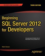
ApressFinancialdatabase, and click the Tables node to expand and list the tables within your database. Find theCustomerDetails.Customerstable, right-click it to bring up the pop-up menu, and select Select Top 1000 Rows. You may recall that the value of 1,000 is arbitrary and is set in the options. This instantly opens up a new Query Editor window pane like the one shown in Figure 10-1, which shows all the rows that are in theCustomerDetails.Customerstable. But how did SQL Server get this data? Let's find out (the secret may already be there, depending on the options for SQL Server).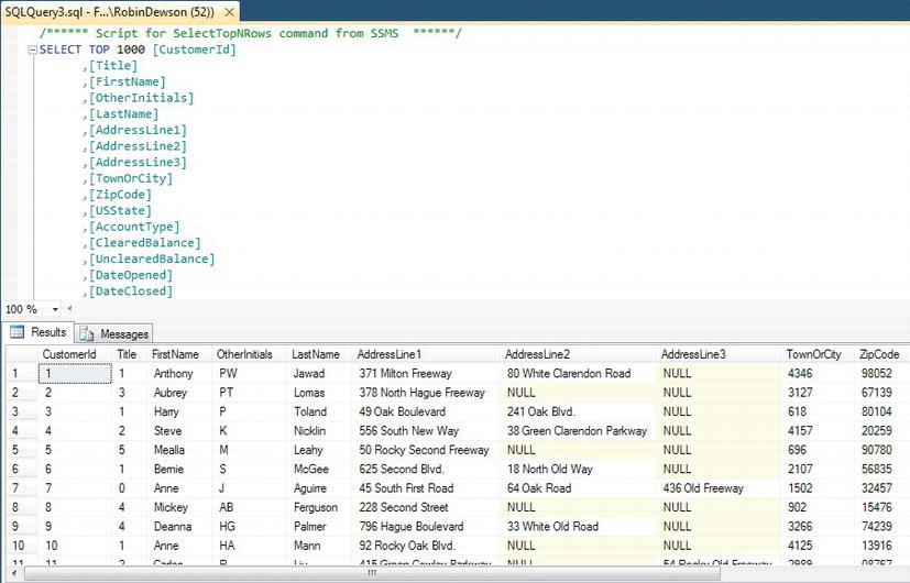
Figure 10-1.
CustomerDetails.Customerstable retrieving data - Above the results, you will see the
SELECTT-SQL statement used to return the data. TheSELECTstatement is returning the top 1,000 rows and then defining the columns to display. - You can alter the number next to the top clause if you want to return a smaller or a greater number of rows, and then re-execute the query. For this first time, alter this to 3, and you should see something similar to Figure 10-2. This will return a maximum of three rows.
Figure 10-2. Three rows returned
If you entered a value of 100 and you had only 20 rows in your table, you would get only 20 rows returned. You would use this perhaps when you didn't know the number of rows within a table, but you were interested only in a maximum number of 100 if there are more. This would be when you wanted to look at just a small selection of content in columns within a table.
Now that you know how to return data from SQL Server Management Studio, let's look in more detail at using T-SQL as well as the T-SQL statement you will probably use most often: SELECT.
Using the SELECT Statement to Retrieve Data
If you wish to retrieve data for viewing from SQL Server using T-SQL statements, then the SELECT statement is the statement you need to use. This is quite a powerful statement, as it can retrieve data in any order, from any number of columns, and from any table that you have the authority to retrieve data from. It can also perform calculations on that data during data retrieval and even include data from other tables! If the user does not have the authority to retrieve data from a table, then you will receive an error message informing the user that permission is denied. SELECT has a lot more power than even the functions mentioned so far, but for the moment, let's concentrate on the fundamentals.
The SELECT Statement
Let's take some time to inspect the simple syntax for a SELECT statement. Square brackets indicate that the phrases are optional, and curly brackets show that at least one of the items must be selected, but there are choices.
SELECT [ ALL | DISTINCT ]

[ TOP expression [ PERCENT ] [ WITH TIES ] ]

    {

                *

      | { table_name | view_name | alias_name }.*

      | { column_name | [ ] expression | $IDENTITY | $ROWGUID }

      [ [ AS ] column_alias ]

      | column_alias = expression

    } [ ,...n ]

[ FROM table_name | view_name alias_name ]

[ WHERE filter_condition ]

[ ORDER BY ordering_criteria ]
The following list breaks down the SELECT syntax, explaining each option. More explanation will be given throughout the chapter as well.
SELECT: Required; this informs SQL Server that aSELECTinstruction is being performed. In other words, you want to return just a set of columns and rows to view.ALL | DISTINCT: Optional; if you want to return either all of the rows or only distinct, or unique, rows. Normally, you do not specify either of these options.TOPexpression/PERCENT/WITH TIES: Optional; you can return the top number of rows, which will be in an arbitrary order unless you order the rows with anORDER BYclause. You can also add the wordPERCENTto the end: this will mean that the top n percent of rows will be returned.WITH TIEScan be used only with anORDER BY. If you specify you want to returnTOP10 rows, and the 11th row has the same value as the 10th row on those columns that have been defined in theORDER BY, then the 11th row will also be returned. It's the same for subsequent rows, until you get to the point that the values differ.*: Optional; by using the asterisk, you are instructing SQL Server to return all the columns from all the tables included in the query. This is not an option that should be used on large amounts of data or over a network. Especially if the network is busy or there are a large number of columns, you really should not use this against production data. By using this, you are bringing back more information than is required. In essence, by using*, you are not in control of the column data you are returning. Wherever possible, you should name the columns instead.table_name.*|view_name.*|alias_name.*: Optional; similar to*, but you are defining which table, if theSELECTis working on more than one table that all the columns from that table will display from. When working with more than one table, this is known as aJOIN, and this option will be demonstrated in Chapter 13 when you take a look at joins, as well as at the end of this chapter.column_name: Optional but recommended; this option is where you name the columns that you wish to return from a table. When naming the columns, it is always a good idea to prefix the column names with their corresponding table names or table alias (more on table alias shortly). This becomes mandatory when you are using more than one table in yourSELECTstatement and instances where there may be columns within different tables that share the same name (preferred to using the alternative*as discussed previously).expression: Optional; you don't have to return columns of rows within aSELECT. You can return a value, a variable, or an expression. If you are usingSELECTfor an expression, then you won't require theFROMkeyword.$IDENTITY: Optional; will return the value from theIDENTITYcolumn.$ROWGUID: Optional; will return the value from theROWGUIDcolumn.AS: Optional; you can change the column header name when displaying the results by using theASoption.Column_alias: Optional; you can give a column name an alias. This is ideal when a column name will form output that is sent to a user. You will see this in Chapter 11 when looking at views.FROM table_name | view_name: Required when selecting data from a data source, optional if you are usingSELECTwith an expression; you will seeSELECTwith expressions in Chapter 13.WHERE filter_condition: Optional; if you want to retrieve rows that meet specific criteria, you need to have aWHEREcondition specifying the criteria to use to return the data. TheWHEREcondition tends to contain the name of a column on the left-hand side of a comparison operator, such as=,<,>, and either another column within the same table, or another table, a variable, or a static value. There are other options that theWHEREcondition can contain, where more advanced searching is required, but on the whole, these comparison operators will be the main constituents of the condition.ORDER BY ordering_criteria: Optional; the data will be returned arbitrarily from the table if noORDER BYexpression is specified. Ascending (ASC) or descending (DESC) is defined for each column, not defined just once for all the columns within theORDER BY. Sorting is completed once the data has been retrieved from SQL Server but before any statement such asTOP. You can also use this expression to return a specific number of rows and subsequent rows after that to enable you to paginate your data and reduce the amount of data returned from a query. You will see this in action later in the chapter.
Keep in mind that when building a SELECT statement, you do not have to name all the columns. In fact, you should retrieve only the columns that you do wish to see; this will reduce the amount of information sent over the network. There is no need to return information that will not be used.
Naming the Columns
When building a SELECT statement, it is not necessary to name every column if you don't want to see every column. You should return only the columns you need. It is very easy to slip into using * to return every column, even when running one-time-only queries. Try to avoid this at all costs; typing out every column name takes time, but when you start dealing with more complex queries and a larger number of rows, the few extra seconds are worth it.
Now that you know not to name every column unless required, and to avoid using *, what other areas do you need to be aware of? First of all, it is not necessary to name columns in the same order that they appear in the table—it is quite acceptable to name columns in any order that you wish. There is no performance hit or gain from altering the order of the columns, but you may find that a different order of the columns might be better for any future processing of the data.
When building a SELECT statement and including the columns, if the final output is to be sent to a set of users, the column names within the database may not be acceptable. For example, if you are sending the output to the users via a file, then they will see the raw result set. Or if you are using a tool such as Crystal Reports to display data from a SELECT statement within a SQL Server stored procedure, then naming the columns would help there as well. The column names are less user-friendly, and some column names will also be confusing for users; therefore, it would be ideal to be able to alter the names of the column headings. Replacing the SQL Server column headings with the new alias column headings desired, in either quotation marks or square bracket delimiters, is easily accomplished with the AS keyword. There is more on this in the next section.
Now that you know about naming the columns, let's take a look at how the SQL statement can return data.
The First Searches
This example will revolve around the CustomerDetails.Customers table, making it possible to demonstrate how all of the different areas mentioned previously can affect the results displayed.
TRY IT OUT: THE FIRST SET OF SEARCHES
- Ensure that Query Editor is running and that you are within the
ApressFinancialdatabase. In the Query Editor pane, enter the following SQL code.Select * From CustomerDetails.Customers - Execute the code using F5, or the execute button on the toolbar. You should then see something like the results shown in Figure 10-3.
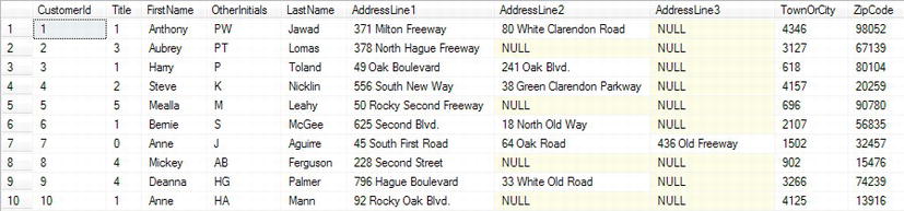
Figure 10-3. Customers table listing all columns (some not shown)
- This is a simple
SELECTstatement returning all the columns and all the rows from theCustomerDetails.Customerstable, as you have just seen. Let's now take it to the next stage, where specific column names will be defined in the query, which is a much cleaner solution and less traffic over a network. - In this instance from the
CustomerDetails.Customerstable, you would like to return a customer's first name, last name, and the current account balances. This would mean namingFirstName,LastName, andClearedBalanceas the column names in the query. The code will read as follows:SELECT firstname,lastname,clearedbalance
FROM CustomerDetails.Customers - Now execute this code, which will return the results shown in Figure 10-4. As you can see, not every column is returned.
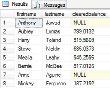
Figure 10-4. Specific columns returned
- As you have seen from the examples so far, the column names, although well named from a design viewpoint, are not exactly suitable if you had to give this data to a set of users.
- Using the same query as before, a couple of minor modifications are required to give the columns aliases. The first alias name is in quotes, as it contains a space. Notice the last column also does not have
ASspecified because this keyword is optional.SELECT FirstName As 'First Name',LastName AS 'Surname',
ClearedBalance Balance
FROM CustomerDetails.Customers - Execute this, and the displayed output changes—it has much friendlier column names, as you see in Figure 10-5.
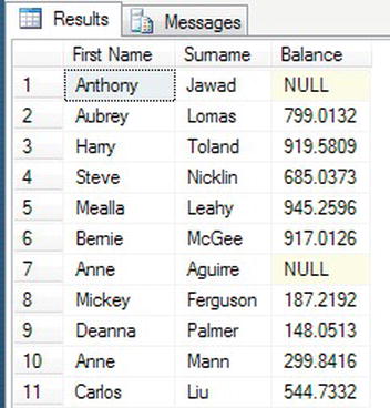
Figure 10-5. Friendly column names
The first SELECT statement demonstrates the fact that in most SQL Server instances, whether you use upper- or lowercase doesn't matter to your queries; however, some language installations are case-sensitive. When installing SQL Server, if you chose a SQL collation sequence that was case-sensitive, as denoted by CS within the suffix of the collation name—SQL_Latin1_General_Cp437_CS_AS, for instance—then the first SELECT query would generate an error. The collation sequence for SQL Server was chosen in Chapter 1 when you installed the application. Changing a collation sequence within SQL Server is a very difficult task that requires rebuilding parts of SQL Server, so this book won't move into that area.
![]() Tip It is strongly recommended, and considered best practice, that you use the correct casing when using queries. Not only does this avoid confusion, but also it means that if you do switch to a case-sensitive installation, then it will not be necessary to alter the query.
Tip It is strongly recommended, and considered best practice, that you use the correct casing when using queries. Not only does this avoid confusion, but also it means that if you do switch to a case-sensitive installation, then it will not be necessary to alter the query.
Let's return to the first query in step 1. This query will select all columns and all rows from the CustomerDetails.Customers table, ordered according to how the database sees it—as you can see in Figure 10-3, it has quite plainly done this.
In the second and third query examples, the columns returned have been reduced to just three columns: the customer's first and last names and the cleared balance amounts. All the rows are still being returned. In the last example, notice that after two of the three columns, there is an AS keyword. This signifies that the following literal is to be used as the column heading; note that if you wish to use two words separated by spaces, you must surround these words by identifiers, whether they be quotation marks, as in your example, or square brackets.
Now that the basics of the SELECT statement have been covered, you will next look at how to display output in different manners within Query Editor.
Varying the Output from a SELECT Query
There are different ways of displaying the output: from a grid, as you have seen; from a straight text file; still within a Query Editor pane; or as pure text. You may have found the results in the previous exercise laid out in a different format than shown previously, depending on how you initially set up Query Editor. In the results of the examples so far, you have seen the data as a grid. This next section will demonstrate tabular text output, otherwise known as Results in Text, as well as outputting the data to a file. Let's get right on with the first option, Results in Text.
TRY IT OUT: PUTTING THE RESULTS IN TEXT AND A FILE
- You should still be in Query Editor. From the Query menu option, select Results To
 Results in Text, or press Ctrl+T. Figure 10-6 shows the other options available from the Results To menu.
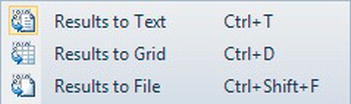
Figure 10-6. Sending the results to different places
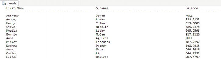
- If you run the same query as step 5 of the preceding example (the code is detailed again here), you will be able to see the difference. Once the code is entered, execute it.
SELECT FirstName As 'First Name',LastName AS 'Surname',

ClearedBalance Balance

FROM CustomerDetails.Customers - Examine the output, which should resemble Figure 10-7. As you can see, the output has changed a great deal. No longer is the output in a nice grid in which the columns have been shrunk to a more manageable size, but each column's data take up, and are displayed to, the maximum number of characters that each column could contain. This obviously stretches out the display, but from here you can see easily how large each column is supposed to be.
- There will be times, though, when users require output to be sent to them. For example, they may wish to know specific details from a set of rows, and so you build a query and save the results to a file to send to them. Or perhaps they want output to perform some analysis of data within a Microsoft Excel spreadsheet.
- To achieve sending output to a file, from the Query menu select Results To Results to File, or by pressing Ctrl+Shift+F. Specify sending results to a file and rerun the code. Once the code has been executed, a Save Results dialog box like the one in Figure 10-8 will appear: this could show any folder location initially—in this case, it shows the folder for results I have set up on my computer.
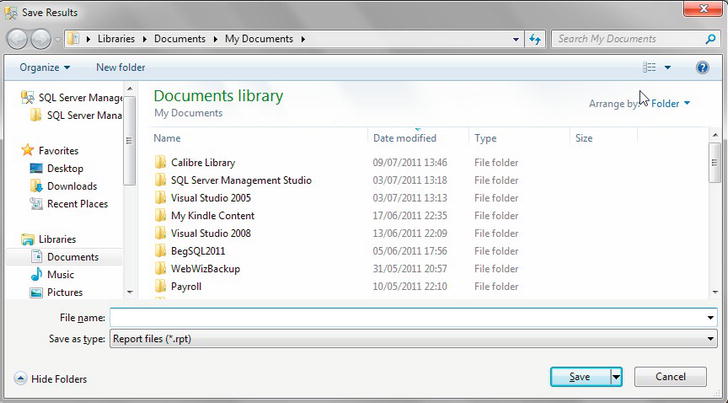
Figure 10-8. Locating where to save the results
- So now that you know how to save to different locations, move back to displaying the output to a grid by pressing Ctrl+D.
![]() Note Before you move on, have you noticed that when you type a query, SQL Server tries to provide you with options about what you may want to use next in your query? This is known as IntelliSense. SQL Server intelligently tries to sense what you may want to have next. You will find that IntelliSense is a very useful tool when building queries, especially, I find, with
Note Before you move on, have you noticed that when you type a query, SQL Server tries to provide you with options about what you may want to use next in your query? This is known as IntelliSense. SQL Server intelligently tries to sense what you may want to have next. You will find that IntelliSense is a very useful tool when building queries, especially, I find, with SELECT queries. If you find it annoying, you can turn it off from Options ![]()
Text Editor ![]()
Transact-SQL/ ![]()
Intellisense.
You now know how to return data, but what happens if you don't want every row and you want to select which rows to display? We'll look at that next.
Limiting a Search: The Use of WHERE
You have a number of different ways to limit the search of rows within a query. Some of the most basic revolve around the three basic relational operators: <, >, and = (less than, greater than, and equal to). There is also the keyword NOT, which could be included with these three operators; however, NOT does not work as in other programming languages that you may have come across: this will be demonstrated within the example in this section so you know how to use the NOT operator successfully.
All of these operators can be found in the WHERE condition of the SELECT statement used to reduce the number of rows returned within a query.
![]() Note You may come across some legacy code in which you will find that the
Note You may come across some legacy code in which you will find that the WHERE condition is used to join two tables together to make the results look as if they came from one table. For some databases, this is the “standard” way to join two tables; however, with SQL Server, the WHERE condition should be used purely as a filter method.
The first exercise will look at how to filter information from your queries, reducing the output to records that you are interested in.
TRY IT OUT: THE WHERE STATEMENT
- The requirement for this section is to find the current share price for Toland's Irish Whisky. This share has a single quotation mark in the name, which would cause issues in the
WHEREcondition if you surrounded the description in single quotation marks. To circumvent this problem, you can setQUOTED_IDENTIFIERto off and then use double quotation marks. You then restrict theSELECTstatement so that only the specific record comes back by using theWHEREcondition, as can be seen in the following code:SET QUOTED_IDENTIFIER OFF
SELECT Description,CurrentPrice
FROM ShareDetails.Shares
WHERE Description = "Toland's Irish Whisky" - Execute this code, and you will see that the single record for ACME is returned, as shown in Figure 10-9.
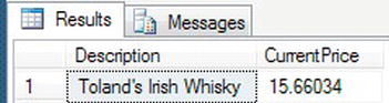
Figure 10-9. The results of limiting the search
- You have seen
WHEREin action using the equals sign; it is also possible to use the other relational operations in theWHEREstatement. The next query demonstrates how SQL Server takes theWHEREcondition and starts returning rows after the given point. This query provides an interesting set of results. Enter the code as detailed here:SET QUOTED_IDENTIFIER OFF
SELECT Description,CurrentPrice
FROM ShareDetails.Shares
WHERE Description >= 'Mackrel Fisheries'
AND Description <= "Toland's Irish" - Once done, execute the code and check the results, which should resemble Figure 10-10. Notice that Toland's Irish Whisky was within the results in step 2 but the value in the “less than or equal to” condition is not listed. There is no row with that exact value within the
ShareDetails.Sharestable. There is a row with most of the text, but not an exact match, and therefore the row is not included. You will come back to this scenario shortly.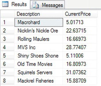
Figure 10-10. Shares output using the
WHEREcondition to filter - The same results can be achieved by using the
BETWEENconditional operator rather than the mathematical operators. The following code will achieve the same results as you have just executed. TheBETWEENoperator indicates to SQL Server to take the two values and find any values including and between the two values provided.SET QUOTED_IDENTIFIER OFF
SELECT Description,CurrentPrice
FROM ShareDetails.Shares
WHERE Description BETWEEN 'Mackrel Fisheries'
AND "Toland's Irish" - Let's now bring in another option in the
WHEREstatement that allows you to avoid returning specific rows. This can be achieved in one of two ways: the first is by using the less than and greater than signs; the second is by using theNOToperator. Enter the following code, which will return all rows except Lomas Ambulances. Run both sets of code at once. This will return two sets of output, known as multiple result sets. I realize there are a lot of rows returned; you will see one method of reducing this in the next section.SET QUOTED_IDENTIFIER OFF
SELECT Description,CurrentPrice
FROM ShareDetails.Shares
WHERE Description <> "Lomas Ambulances"
SELECT Description,CurrentPrice
FROM ShareDetails.Shares
WHERE NOT Description = "Lomas Ambulances" - Executing this code will produce the output shown in Figure 10-11. Notice how in neither set of output ACME has been listed (due to page limitations within the book, only some of the output is within the figure).
- I mentioned in Chapter 9 that you would return to the
WHEREcondition forDELETEstatements. Filtering for deletions is the same as filtering forSELECTstatements. Before executing aDELETE, I tend to build aSELECTstatement, check that the data to delete is correct and then switch theSELECTto aDELETE. TheDELETEcode here has twoWHEREconditions to limit the number of deletions to one year of data and where the price is greater than 6 trillion.DELETE
FROM ShareDetails.SharePrices
WHERE PriceDate BETWEEN '1 Jan 2012' and '3 Jan 2012'
AND Price > 23.00
As you have seen, it is possible to limit the number of rows to be returned via the WHERE condition; you can return rows up to a certain point, after a certain point, or even between two points with the use of an AND or BETWEEN expression. It is also possible to exclude rows that are not equal to a specific value or range of values by using the NOT expression or the <> operator.
When the SQL Server data engine executes the T-SQL SELECT statement, it is the WHERE condition that is dealt with before any ordering of the data, or any limitation placed on it concerning the number of rows to return. The data are inspected, where possible using an index, to determine whether a row stored in the relevant table matches the selection criteria within the WHERE condition, and if it does, to return it. If an index cannot be used, then a full table scan will be performed to find the relevant information.
Table scans can present a large performance problem within your system, and you will find that if a query has to perform a table scan, then data retrieval could be very slow, depending on the size of the table being scanned. If the table is small with only a small number of rows, then a table scan is likely to retrieve data more quickly than the use of an index. However, table scanning and the speed of data retrieval will be the biggest challenge you will face as a SQL Server developer. With data retrieval, it is important to bear in mind that whenever possible, if you are using a WHERE condition to limit the rows returned, you should try to specify the columns from an index definition in this WHERE condition. By doing this, you will be giving the query the best chance for optimum performance.
As discussed in Chapter 6, getting the index right is crucial to fast data manipulation and retrieval. If you find you are forever placing the same columns in a WHERE condition, but those columns do not form part of an index, perhaps this is something that should be revisited to see whether any gain can come from having the columns be part of an index.
For any table, ensuring that the WHERE condition is correct is important. As has been indicated from a speed perspective, using an index will ensure a fast response of data. This gains greater importance with each table added, and even more importance as the size of each table grows.
Finally, by ensuring the WHERE condition filters out the correct rows, you will ensure that the required data are returned, the right results are displayed, and smaller amounts of data are sent across the network, as the processing is done on the server and not the client. Also, having the appropriate indexing strategy helps with this as well.
It is also possible to return a specific number of rows, or a specific percentage of the number of rows, as you saw when displaying rows in SQL Server Management Studio. These statements are discussed next, with a short code example demonstrating each in action. First of all, you will look at a statement that does not actually form part of the SELECT statement itself.
TOP n
This option, found within the SELECT statement itself, will return a specific number of rows from the SELECT statement, and is very much like the SET ROWCOUNT function that you will see shortly. In fact, the TOP n option is the preferred option to use when returning a set number of rows, as opposed to the SET ROWCOUNT function. The reason behind this is that TOP n applies only to the query statement that includes it; however, by using SET ROWCOUNT n, you are altering all executions until you reset SQL Server to act on all rows through SET ROWCOUNT 0.
Although it is possible to use TOP n without any ORDER BY statement, it is usual to combine TOP with ORDER BY. When no order is specified, the rows returned are arbitrary, and if you want consistent results, then ordering will provide this. If you are not concerned about which rows are returned, then you can avoid using ORDER BY. TOP n will still return and display the top n rows in an arbitrary order.
Any WHERE statements and ORDER BY statements within the SELECT statement are dealt with first, and then, from the resultant rows, the TOP n function comes into effect. This then allows the correct number of rows to be displayed as opposed to finding the number of rows from the TOP n function, then filtering the rows using the WHERE statement as the filter could make the number of rows from the ones selected to be zero.
The use of WHERE and ORDER BY will be demonstrated with the following example.
TRY IT OUT: TOP N
- In Query Editor, enter the following code into a new Query Editor pane:
SELECT TOP 3 *

FROM ShareDetails.Shares

WHERE CurrentPrice > 20

ORDER BY Description - Once entered, execute the code. It returns a result set, as shown in Figure 10-12, with three rows of data. SQL Server looked for rows where the
CurrentPricewas greater than 20, then ordered the results, and finally displayed the top 3 of the result set.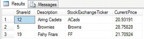
Figure 10-12. Top three rows after filter and sort
You could run the code in step 1 without the ORDER BY, which will show you a different three rows returned.
TOP n PERCENT
TOP n PERCENT is very similar to the TOP n clause with the exception that instead of working with a precise number of rows, it is a percentage of the number of rows that will be returned. Keep this in mind, as it is not a percentage of the number of rows within the table. Also, the number of rows is rounded up; therefore, as soon as the percentage moves over to include another row, then SQL Server will include this extra row.
You see more of this option in Chapter 11, which discusses the building of views.
SET ROWCOUNT n
SET ROWCOUNT n is a totally separate statement from the SELECT statement and can be used with other statements within T-SQL. What this statement will do is limit or reset the number of rows that will be processed for the session that the statement is executed in.
![]() Note Caution should be exercised if you have any statements that also use a
Note Caution should be exercised if you have any statements that also use a TOP statement, described next.
The SET ROWCOUNT n statement stops the processing of the SELECT statement once the number of rows defined has been reached. The difference between SET ROWCOUNT and SELECT TOP n is that the latter will perform one more internal instruction than the former. Processing halts immediately when the number of rows processed through SET ROWCOUNT is reached. However, by using the TOP statement, all the rows are returned internally, the TOP n rows are selected from that group internally, and these are then passed for display. Returning a limited number of rows is useful when you want to look at a handful of data to see what values could be included, or perhaps you wish to return a few rows for sampling the data.
You can set the number of rows to be affected by altering the number, n, at the end of the SET ROWCOUNT statement. This setting will remain in force only within the query window in which the statement is executed, or within the stored procedure in which the statement is executed. It will also remain in force in that query window until you alter the value. This is not a temporary setting per se.
To reset the session so that all rows are taken into consideration, you would set the ROWCOUNT number to 0.
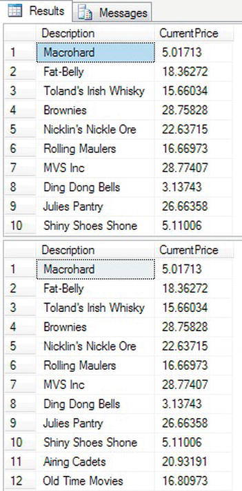
TRY IT OUT: SET ROWCOUNT
- In Query Editor, enter the following code into a new Query Editor pane:
SET ROWCOUNT 3

SELECT * FROM ShareDetails.Shares

SET ROWCOUNT 0

SELECT * FROM ShareDetails.Shares - Once it is entered, execute it. You should see two result sets, as shown in Figure 10-13. The first will return three rows from the
ShareDetails.Sharestable. The second result set will return all rows fromShareDetails.Shares.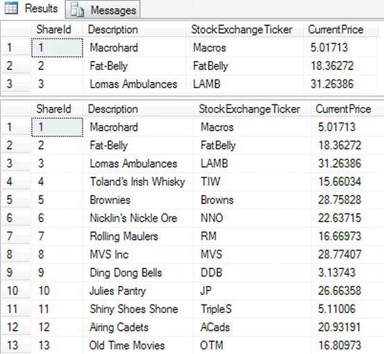
- The final example will combine
ROWCOUNTandTOP nin an example showing how these two statements can alter your results. Enter the following code.SET ROWCOUNT 3
SELECT TOP 2 *
FROM ShareDetails.Shares
WHERE CurrentPrice > 20
ORDER BY Description
SET ROWCOUNT 2
SELECT TOP 3 *
FROM ShareDetails.Shares
WHERE CurrentPrice > 20
ORDER BY Description
SET ROWCOUNT 0
SELECT TOP 3 *
FROM ShareDetails.Shares
WHERE CurrentPrice > 20
ORDER BY Description - When you execute the code, you should see three result sets, as shown in Figure 10-14.
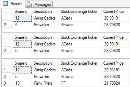
Figure 10-14. Three results sets demonstrating
ROWCOUNTandTOP N - The first result set is limited by the
TOP 2expression within theSELECT. As long as theROWCOUNTstatement had a value that was the same as or greater than theTOPexpression, then two rows would be returned. Looking at the second result set, you will see that theROWCOUNTstatement is in control of the number of rows returned this time. Finally the third result set will return the number of rows from theTOPexpression.
String Functions
A large number of system functions are available for manipulating data. This section looks purely at the string functions available for use within a T-SQL statement; later in the book, you will look at some more functions that are available. Following are the functions that are used in the next example:
LTRIM/RTRIM: These perform similar functionality. If you have a string with leading spaces, and you wish to remove those leading spaces, you would useLTRIMso that the returnedvarcharvalue would have a nonspace character as its first value. If you have trailing spaces, you would useRTRIM. You can use this function only with a data type ofvarcharornvarchar, or a data type that can be implicitly converted to these two data types, or with a data type converted tovarcharornvarcharusing theCASTSQL Server function.CAST: This specialized function converts one data type to another data type. This is not specifically a string function as you can cast from a string to a numeric; however, the casting into a string is more common as it can be used to cast a number into a string, which is then concatenated into several strings.LEFT/RIGHT: This function returns the leftmost or rightmost characters from a string. Passing in a second parameter to the function will determine the number of characters to return from whichever side of the string. TheLEFTandRIGHTfunctions accept any data type excepttextorntextexpressions to perform the string manipulation, implicitly converting any noncharacter data type orvarcharornvarchar, and returning avarcharornvarchardata type as a result.
It is possible to do more than just return columns. Columns can have further functionality applied to them. In the following example, some basic string functions will be shown. You will see more manipulation of information in Chapter 13.
TRY IT OUT: STRING FUNCTIONS
- Enter the code that follows into an empty Query Editor window. Alter the output to text format by pressing Ctrl+T. Notice the use of the
+operator within theSELECTquery. This will concatenate the strings defined within the query into one single string value. Note Unlike with some programming languages, you cannot use the
 &character, as this has a totally different meaning in SQL Server. It is used for bitwise operations.SELECT FirstName + ' ' + LastName +
' has a cleared balance of $' +
CAST (ClearedBalance AS varchar(40))
FROM CustomerDetails.Customers
WHERE FirstName = 'Aubrey' - Execute this code, which produces the output shown in Figure 10-15.
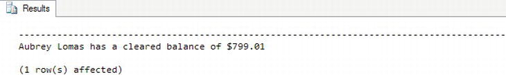
Figure 10-15. Concatenating results
- As you can see, it's a bit unwieldy. The
Namecolumn heading goes far wider than is required. There is a complex way of getting this right, but a much simpler method is to use theLEFTstatement. The sum of the width of the three columns gives this column width displayed in the output; by using theLEFTstatement, it is possible to achieve something better. Clear the Query Editor pane, and enter the following code: - Execute the preceding code. This produces the results shown in Figure 10-16. What the preceding query has done is to reduce the output to the first 50 characters starting from the left.
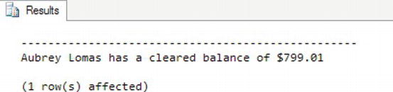
Figure 10-16. Concatenating results and reducing the width
- The best way is to remove all trailing spaces rather than guesstimate how wide to make the string is the
RTRIMstatement. The following code does this, although the output in the text layout doesn't. This is because SQL Server still doesn't know what the maximum size of the concatenation will be, and it has to believe that the maximum number of characters of the sum of the two columns could still be displayed. However, in truth, the amount of data returned will be minimal. Therefore, this is a great method of reducing the amount of data passed over a network.SELECT RTRIM(FirstName + ' ' + LastName +
' has a cleared balance of $' +
CAST (ClearedBalance AS varchar(40)))
FROM CustomerDetails.Customers
WHERE FirstName = 'Aubrey'
In all of the examples thus far, rows are returned in an arbitrary order. You look now at how this can be changed.
Order! Order!
Of course, retrieving the rows in any order SQL Server desires may not always be what you desire. However, it is possible to change the order in which you return rows. This is achieved through the ORDER BY clause, which is part of the SELECT statement. The ORDER BY clause can have multiple columns, even with some being in ascending order and others in descending order.
If you should find that you are repeatedly using the same columns within an ORDER BY clause, or that the query is taking some time to run, you should consider having the columns within the query as an index. (Indexes were covered in Chapter 6.)
Ordering the data will of course increase processing time, but it is used as a necessity to display the data in the correct order. Ordering on varchar columns also takes longer than numeric columns.
The ORDER BY clause also has the option to allow you to paginate your data, which is ideal if you are creating a SELECT statement to return rows to display in a screen. There are two options that are required, and they are OFFSET and FETCH NEXT. The first option determines the number of rows to skip before returning data, and the latter option determines the number of rows to return. You will see a demonstration of this in the following section, and it will be demonstrated in action in Chapter 16.
![]() Note Ordering takes place after the filtering of rows but before the
Note Ordering takes place after the filtering of rows but before the TOP statement, so you could still be ordering a large set of rows before returning the top few you may need.
Let's now take a look at building a query that uses an ORDER BY clause.
TRY IT OUT: ALTERING THE ORDER
- Clear the query window in Query Editor, and set the display option back to showing a grid by selecting, from the Query menu, Results To Results to Grid. Once complete, enter the following code into the Query Editor pane. This will return the data in the ascending (the default) order of the cleared balance of your customers for those customers who have a cleared balance value.
SELECT LEFT(FirstName + ' ' + LastName,50) AS 'Name',

ClearedBalance Balance

FROM CustomerDetails.Customers

WHERE ClearedBalance IS NOT NULL

ORDER BY Balance - Execute the code; this will produce the results shown in Figure 10-17.
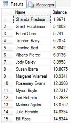
Figure 10-17. Altering the order by balance and ignoring
NULLvalues - You can also complete the same query, but have the cleared balance in descending order rather than ascending order. This is simply done by placing
DESCafter the column name. Change your code as detailed here:SELECT LEFT(FirstName + ' ' + LastName,50) AS 'Name',
ClearedBalance Balance
FROM CustomerDetails.Customers
WHERE ClearedBalance IS NOT NULL
ORDER BY Balance DESC - Execute the code; this will produce the results shown in Figure 10-18.
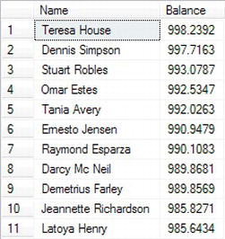
Figure 10-18. Making the order in descending sequence
- To paginate your data, there are three elements that have to be included in your
SELECTstatement:• The first element is the
ORDER BY. This is so that SQL Server will know the order in which the data will be returned will be as constant as possible. The caveat of “as possible” is because data may be added to the table between calls to display the paginated data.• The second element is the
OFFSETclause, which determines the number of rows to skip before returning the data.• The final element is the number of rows to return.
- To return the first four rows from
CustomerDetails.Customers, then theOFFSETwould be zero andFETCH NEXThas a value of 4. Enter this code:SELECT LEFT(FirstName + ' ' + LastName,50) AS 'Name',
ClearedBalance Balance
FROM CustomerDetails.Customers
WHERE ClearedBalance IS NOT NULL
ORDER BY Balance
OFFSET 0 ROWS
FETCH NEXT 4 ROWS ONLY - Now execute the code. Figure 10-19 shows the first four rows returned.
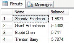
Figure 10-19. Using
OFFSETandFETCH NEXTto return rows - To return the next set of four rows, enter the following code. You may think that hard-coding the number for the starting position is not the correct method because the
OFFSETwill increase with each call. You would use a locally defined variable.SELECT LEFT(FirstName + ' ' + LastName,50) AS 'Name',
ClearedBalance Balance
FROM CustomerDetails.Customers
WHERE ClearedBalance IS NOT NULL
ORDER BY Balance
OFFSET 4 ROWS
FETCH NEXT 4 ROWS ONLY - When you execute the foregoing code, you will see results similar to Figure 10-20.
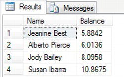
Figure 10-20. Using
OFFSETandFETCH NEXTto subsequent rows
The LIKE Operator
It is possible to use more advanced techniques for finding rows where a mathematical operation doesn't quite fit; for example, say someone is trying to track down a customer, but doesn't know the customer's full name, or does know the first part of his or her surname but doesn't know how to spell the full name.
Suppose you know that the surname ends in “Smith” but you cannot recall the first part of the surname. So how would this be put into a query? There is a keyword that you can use as part of the WHERE statement, called LIKE. This will use pattern matching to find the relevant rows within a SQL Server table using the information provided.
The LIKE operator can come with one of four operators, which are used alongside string values that you want to find. Each of the four specifiers is detailed in the following list. They can be used together, and using one does not exclude using any others.
%: This would be placed at the end and/or the beginning of a string. The best way to describe this is through an example; if you were searching the customers who had the letter “a” within their surname, you would search for “%a%”, which would look for the letter “a,” ignoring any letters before and after the letter “a”, and just checking for that letter within the first name column._: This looks at a string, but only for a single character before or after the position of the underscore. Therefore, looking in the first name column for “_a” would return any customer who has two letters in his or her first name where the second letter is an “a.” In the example, no rows would be returned. However, if you combined this with the % sign and searched for “_a%,” then you would get back Jason Atkins, Ian McMahon, and Ian Prentice. You would not get back Vic McGlynn, because “a” is not the second letter.[]: This lets you specify a number of values or a range of values to look for. For example, if you were looking in the player's first name for the letters “c-f,” you would useLIKE"%[c-f]%".[^...]: Similar to the preceding option, this one lists those items that do not have values within the range specified.
![]() Note
Note LIKE is not case-sensitive unless you have the SQL Server instance set to a collation that is case-sensitive.
The best way to learn how to use LIKE is to see an example.
TRY IT OUT: THE LIKE OPERATOR
- We are going to try to find Mark Vernon-Smith via the
LastNamecolumn. You know the name ends with Smith and the surname is hyphenated. The code that follows will search all of the customer rows looking for anything prefixing -Smith.SELECT FirstName + ' ' + LastName
FROM CustomerDetails.Customers
WHERE CustomerLastName LIKE '%-Smith' - Execute the code; this will give the results shown in Figure 10-21.
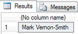
Figure 10-21. Using the
LIKEoperator - You can also go to extremes using the
LIKEoperator—for example, seeing which customers have the letter “q” anywhere in their name. The code for this is shown here:SELECT FirstName + ' ' + LastName AS [Name]
FROM CustomerDetails.Customers
WHERE FirstName + ' ' + LastName LIKE '%q%' - When you execute this, you should get the results shown in Figure 10-22: 13 customers are returned, as they have a “q” somewhere in their name.
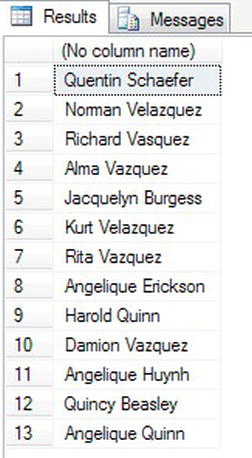
Figure 10-22. Using
LIKEto search for customers with “q” in their name - Why would you want to go to such lengths of concatenating the names? Would it not have been possible to use the Name alias, which is a combination of the first name and last name columns? Well, unfortunately not—the code you might expect to use would look something like the following. Enter this code:
SELECT FirstName + ' ' + LastName AS [Name]

FROM CustomerDetails.Customers

WHERE [Name] LIKE '%q%' - Execute this code. Instead of the success messages that you have become used to, an error message will be returned. You can search only on real column names, not aliases.
Msg 207, Level 16, State 1, Line 3

Invalid column name 'Name'.
![]() Note There may be times that you'll want to take data from a table in one database on one server and insert the data into another table in another database on another server. A typical scenario might be when data have been inadvertantly deleted, but you have a backup on another database. By using a
Note There may be times that you'll want to take data from a table in one database on one server and insert the data into another table in another database on another server. A typical scenario might be when data have been inadvertantly deleted, but you have a backup on another database. By using a SELECT statement and many string actions, it is possible to build up a result set of INSERT statements. You can then store these to a text file, which you can use to run against in another database. A short code example would be:
SELECT "INSERT (Column1) VALUES ("'+column1+"'") FROM Table1
Creating Data: SELECT INTO
It's time now to start getting into a more advanced topic of SELECT. It is possible to create a new table within a database by using the INTO keyword, like that found in INSERT INTO, within a SELECT statement, provided, of course, you have the right database permissions to create tables in the first place.
First, it is necessary to clarify the syntax of how the SELECT INTO statement is laid out; you simply add the INTO clause after the column names, but before the FROM keyword. Although the following section of code shows just one table name, it is possible to create a new table from data from one or more tables.
SELECT *|column1,column2,...

INTO new_tablename

FROM tablename
The INTO clause is crucial to the success of the creation of the new table. The SELECT statement will fail if there is a table already in existence with the same name for the same table owner. This will be demonstrated within the example in this section. You tend to use this statement to create a temporary table in tempdb, although you can use it to build a table in your database.
The table generated will consist of the columns returned from the built SELECT statement, whether that is all the columns from the table mentioned within the FROM statement or a subset. The new table will also contain only the rows returned from the SELECT statement. To clarify, this statement is creating a new table using the structure within the SELECT statement. There will be no keys, constraints, relationships, or in fact any other facet of SQL Server, except a new table. Hence, creating tables using SELECT...INTO should be done only with care.
Two tables can exist with the same name within a database, providing that they have different schemas. The tables in ApressFinancial all have the database owner as their owner, but it is possible for a CustomerDetails.Customers table to exist for an owner like StepBrow.
![]() Note Although possible, having two tables of the same name but different owners is not recommended, as it causes confusion.
Note Although possible, having two tables of the same name but different owners is not recommended, as it causes confusion.
Let's look at the INTO statement in action.
- In an empty Query Editor window, enter the following code:
SELECT FirstName + ' ' + LastName AS [Name],

ClearedBalance,UnclearedBalance

INTO CustTemp

FROM CustomerDetails.Customers - Execute the code. This will return the following message in the results pane:
(1000 row(s) affected)
- If you now move to Object Explorer on the left-hand side (if Object Explorer is no longer there, press F8) and complete a refresh, you should see a new table in the expanded Tables node, called
dbo.CustTemp, as shown in Figure 10-23.
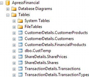
Figure 10-23. New table created with SELECT INTO
You should use the INTO clause with care. For instance, in this example, security has not been set up for the table, and you are also creating tables within your database that have not been through any normalization or development life cycle. It is also very easy to fill up a database with these tables if you are not careful. However, it is a useful and handy method for taking a backup of a table and then working on that backup while testing out any queries that might modify the data. Do ensure, though, that there is enough space within the database before building the table if you do use this technique.
![]() Note It is best to avoid using
Note It is best to avoid using SELECT INTO in a production environment unless you really do need to keep the table permanently. Also take note that the table in the previous “Try It Out” exercise was placed in the CustomerDetails schema. You may want to create a special schema for tables created using SELECT INTO if they are not permanent additions to your database. You may find, though, that it is better to use the temporary database, tempdb, as a place to put tables created using SELECT INTO, especially if they are going to exist for only a short period of time. The ”Try It Out” code would then read as follows:
SELECT CustomerFirstName + ' ' + CustomerLastName AS [Name],

ClearedBalance,UnclearedBalance

INTO CustomerDetails.CustTemp

FROM CustomerDetails.Customers
Updating Data
Now that data has been inserted into your database, and you have seen how to retrieve this information, it is time to look at how to modify the data, referred to as updating the data.
Ensuring that you update the right data at the right time is crucial to maintaining data integrity. You will find that when updating data, and also when removing or inserting data, it is best to group this work as a single, logical unit, within a transaction, thereby ensuring that if an error does occur, it is still possible to return the data back to its original state. You were first introduced to transactions in Chapter 9, and I will be building on your knowledge to cover nesting of transactions.
First of all, let's take a look at the syntax for the UPDATE statement.
The UPDATE Statement
The UPDATE statement will update columns of information on rows within a single table returned from a query that can include selection and join criteria. The syntax of the UPDATE statement has similarities to the SELECT statement, which makes sense, as it has to look for specific rows to update, just as the SELECT statement looks for rows to retrieve. You will also find that before doing updates, especially more complex updates, you need to build up a SELECT statement first and then transfer the JOIN and WHERE details into the UPDATE statement. The syntax that follows is in its simplest form. Once you become more experienced, the UPDATE statement can become just as complex and versatile as the SELECT statement.
UPDATE

    [ TOP ( expression ) [ PERCENT ] ]

    [[ server_name . database_name . schema_name .

    | database_name .[ schema_name ] .

    | schema_name .]

table_or_viewname

    SET

        { column_name = { expression | DEFAULT | NULL }

          | column_name { .WRITE ( expression , @Offset , @Length ) }

          | @variable = expression

          | @variable = column = expression [ ,...n ]

        } [ ,...n ]

    [FROM { <table_source> } [ ,...n ] ]

    [ WHERE { <search_condition>]
The first set of options you know from the SELECT statement. The tablename clause is simply the name of the table on which to perform the UPDATE. Moving on to the next line of the syntax, you reach the SET clause. It is in this clause that any updates to a column take place. One or more columns can be updated at any one time, but each column to be updated must be separated by a comma.
When updating a column, there are four choices that can be made for data updates. Updates can be through the following:
- A direct value setting
- A section of a value setting providing that the recipient column is
varchar,nvarchar, orvarbinary - The value from a variable
- A value from another column, even from another table
You can even have mathematical functions or variable manipulations included in the right-hand clause, have concatenated columns, or have manipulated the contents through STRING, DATE, or any other function. The update will be successful as long as the result's left-hand side and right-hand side both have the same data type. As a result, you cannot place a character value into a numeric data type field without converting the character to a numeric value.
If you are updating a column with a value from another column, the only value that it is possible to use is the value from the same row of information in another column, provided this column has an appropriate data type. When I say “same row,” remember that when tables are joined together, this means that values from these joined tables can also be used as they are within the same row of information. Also, the expression could be the result of a subquery.
![]() Note A subquery is a query that sits inside another query. You look at subqueries in Chapter 13.
Note A subquery is a query that sits inside another query. You look at subqueries in Chapter 13.
The FROM table source clause will define the table(s) used to find the data to perform the update on the table defined next to the UPDATE statement. Like SELECT statements, it is possible to create JOIN statements; however, you must define the table you are updating within the FROM clause.
Finally, the WHERE condition is exactly as in the SELECT statement, and can be used in exactly the same way. Note that omitting the WHERE clause will mean the UPDATE statement will affect every row in the table.
Updating Data Within Query Editor
To demonstrate the UPDATE statement, the first update to the data will be to change the name of a customer, replicating when someone changes his or her name due to marriage or deed, for example. This uses the UPDATE statement in its simplest form, by locating a single record and updating a single column.
TRY IT OUT: UPDATING A ROW OF DATA
- Ensure that Query Editor is running and that you are logged in with an account that can perform updates. In the Query Editor pane, enter the following
UPDATEstatement:USE ApressFinancial
GO
UPDATE CustomerDetails.Customers
SET LastName = 'Mather'
WHERE CustomerId = 7 - It is as simple as that! Now that the code is entered, execute the code, and you should then see a message like this:
(1 row(s) affected)
- Now enter a
SELECTstatement to check that Customer Id 7 is now Anne Mather. For your convenience, here's the statement, and the results are shown in Figure 10-24.SELECT FirstName + ' ' + LastName
FROM CustomerDetails.Customers
WHERE CustomerId = 7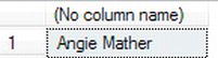
Figure 10-24. Updating the surname of one customer
- Now here's a little trick that you should know, if you haven't stumbled across it already. If you check out Figure 10-25, you will see that the
UPDATEcode is still in the Query Editor pane, as is theSELECTstatement. No, you aren't going to perform theUPDATEagain! If you highlight the line with theSELECTstatement by holding down the left mouse button and dragging the mouse, then only the highlighted code will run when you execute the code again.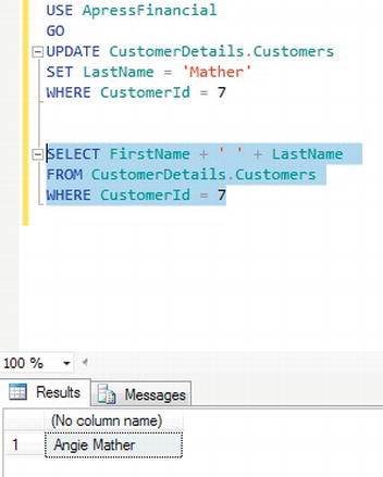
- On executing the highlighted code, you should see only the values returned for the
SELECTstatement as you saw previously, and no results saying that an update has been performed.
Updating Data from a Variable or Another Column
It is also possible to update data using information from another column within the table, or with the value from a variable. This next example will demonstrate how to update a row of information using the value within a variable, and a column from the same table. Notice how although the row will be found using the LastName column, the UPDATE statement will also update that column with a new value. To define a variable, you have to use the DECLARE statement and any variable name needs to start with one @ sign for local variables and two @@ signs for global variables. A local variable is a variable that has a lifetime of the query that contains it; a global variable has a lifetime of the query that contains it, as well as any other query while the declaration query is active. You will see more on these in Chapter 13. Enter the following code and then execute it:
SELECT FirstName,LastName,ClearedBalance,UnclearedBalance

FROM CustomerDetails.Customers

WHERE lastname = 'Booth'


DECLARE @ValueToUpdate VARCHAR(30)

SET @ValueToUpdate = 'Prentice'

UPDATE CustomerDetails.Customers

   SET LastName = @ValueToUpdate,

       ClearedBalance = ClearedBalance + UnclearedBalance ,

       UnclearedBalance = 0

 WHERE LastName = 'Booth'


SELECT FirstName,LastName,ClearedBalance,UnclearedBalance

FROM CustomerDetails.Customers

WHERE lastname = 'Prentice'
You should then see the output shown in Figure 10-26.
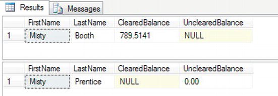
Figure 10-26. Showing the values of the customer before and after the update
Updating a Column with Different Data Types
Now let's move on to updating columns in which the data types don't match. SQL Server does a pretty good job when it can to ensure the update occurs, and these following examples will demonstrate how well SQL Server copes with updating an integer data type with a value in a varchar data type.
- The first example will demonstrate where a
varcharvalue will successfully update a column defined asint. Enter the following code:SELECT FirstName,LastName,ClearedBalance,UnclearedBalance
FROM CustomerDetails.Customers
WHERE lastname = 'Prentice'
DECLARE @ValueToUpdate VARCHAR(30)
SET @ValueToUpdate = '1422.26'
UPDATE CustomerDetails.Customers
SET ClearedBalance = @ValueToUpdate
WHERE LastName = 'Prentice'
SELECT FirstName,LastName,ClearedBalance,UnclearedBalance
FROM CustomerDetails.Customers
WHERE lastname = 'Prentice' - Execute the code; you should see the output shown in Figure 10-27, where the
ClearedBalancebecomes 1422.26. SQL Server has performed an internal data conversion (known as an implicit data type conversion) and has come up with amoneydata type from the value withinvarchar, as this is what the column expects, and therefore can successfully update the column.
Figure 10-27. Showing the values of the customer before and after the update
- However, in this next example, the data type that SQL Server will come up with is a numeric data type. When you try to alter an integer-based data type,
bigint, with this value, which you can find in theAddressIdcolumn, theUPDATEdoes not take place. Enter the following code:SELECT FirstName,LastName,ClearedBalance,UnclearedBalance
FROM CustomerDetails.Customers
WHERE lastname = 'Prentice'
DECLARE @ValueToUpdate VARCHAR(30)
SET @ValueToUpdate = 'Invalid'
UPDATE CustomerDetails.Customers
SET ClearedBalance = @ValueToUpdate
WHERE LastName = 'Prentice'
SELECT FirstName,LastName,ClearedBalance,UnclearedBalance
FROM CustomerDetails.Customers
WHERE lastname = 'Prentice' - Now execute the code. Notice when you do that SQL Server generates an error message informing you of the problem. Hence, never leave data conversions to SQL Server to perform and convert the data explicitly. Try to get the same data type updating the same data type. You look at how to convert data further to the
CASTstatement in Chapter 14.
(1 row(s) affected)


Msg 235, Level 16, State 0, Line 8

Cannot convert a char value to money. The char value has incorrect syntax.
Updating data can be very straightforward, as the preceding examples have demonstrated. Where at all possible, use a unique identifier—for example, the CustomerId—when trying to find a customer, rather than a name. There can be multiple rows for the same name or other type of criteria, but by using the unique identifier, you can be sure of using the right record every time. To place this in a production scenario, you would have a Windows-based graphical system that would allow you to find details of customers by their name, address, or account number. Once you found the right customer, instead of keeping those details to find other related rows, you would keep a record of the unique identifier value instead.
Returning to the UPDATE statement and how it works, first of all SQL Server will filter out from the table the first row that meets the criteria of the WHERE statement. The data modifications are then made, and SQL Server moves on to try to find the second row matching the WHERE statement. This process is repeated until all the rows that meet the WHERE condition are modified. Therefore, if using a unique identifier, SQL Server will update only one row, but if the WHERE statement looks for rows that have a LastName of Dewson, multiple rows could be updated (Robin and Julie). So choose your row selection criteria for updates carefully.
But what if you didn't want the update to occur immediately? There will be times when you will want to perform an update, and then check that the update is correct before finally committing the changes to the table. Or when doing the update, you'll want to check for errors or unexpected data updates. This is where transactions come in, and these are covered next.
Updating Data: Using Transactions
Now, what if, in the first update query of this chapter, you had made a mistake or an error occurred? For example, say you chose the wrong customer, or even worse, omitted the WHERE statement, and therefore all the rows were updated. These are unusual but not uncommon errors, and are quite possible. More common errors could result when more than one data modification has to take place and succeed, and the first one succeeds but a subsequent modification fails. By using a transaction, you would have had the chance to correct any mistakes easily, and could then revert to a consistent state. Of course, this next example is nice and simple, but by working through it, the subject of transactions will hopefully become a little easier to understand and appreciate.
TRY IT OUT: USING A TRANSACTION
- Make sure Query Editor is running for this first example, which will demonstrate
COMMIT TRANin action. There should be no difference from anUPDATEwithout any transaction processing, as it will execute and update the data successfully. However, this should prove to be a valuable exercise, as it will also demonstrate the naming of a transaction. Enter the following code:SELECT 'Before',ShareId, Description,CurrentPrice
FROM ShareDetails.Shares
WHERE ShareId = 3
BEGIN TRAN ShareUpd
UPDATE ShareDetails.Shares
SET CurrentPrice = CurrentPrice * 1.1
WHERE ShareId = 3
SELECT 'During',ShareId, Description,CurrentPrice
FROM ShareDetails.Shares
WHERE ShareId = 3
ROLLBACK TRAN
SELECT 'After',ShareId, Description,CurrentPrice
FROM ShareDetails.Shares
WHERE ShareId = 3 - Notice in the preceding code that
ROLLBACK TRANdoes not use the name associated withBEGIN TRAN. The label afterBEGIN TRANis simply that, a label, and it performs no functionality. It is therefore not necessary to then link up with a similarly labeledROLLBACK TRAN. - Execute the code. Figure 10-28 shows the results, which list out the
Sharestable before and after the update within the transaction, as well as the value after the rollback, to show that the data change has not been committed to the table. This is a straightforward test of your code before update.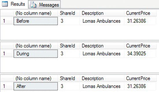
Figure 10-28. Updating with a transaction label and a
ROLLBACK TRAN - However, if instead your code was as shown here, where within the
UPDATEstatement you forgot theShareIdfilter in theWHEREexpression, commented out with two dashes (–), you can see how building your code in a transaction with aROLLBACKbecomes important and would avoid a potentially catastrophic error.
SELECT 'Before',ShareId,ShareDesc,CurrentPrice

  FROM ShareDetails.Shares

 WHERE ShareId = 3

BEGIN TRAN ShareUpd

UPDATE ShareDetails.Shares

   SET CurrentPrice = CurrentPrice * 1.1

-- WHERE ShareId = 3

SELECT 'Within the transaction',ShareId,ShareDesc,CurrentPrice

  FROM ShareDetails.Shares

ROLLBACK TRAN

SELECT 'After',ShareId,ShareDesc,CurrentPrice

  FROM ShareDetails.Shares

 WHERE ShareId = 3
One final point to note: In Chapter 9, I said, “In reality, minimal data are logged about what data pages have been deallocated and therefore removed from the database.” This was followed by the cautionary note that there was no going back on a TRUNCATE outside of a transaction. However, there is the ability to roll back a TRUNCATE within a transaction. A TRUNCATE indicates within the transaction log the data pages that are to be deallocated within SQL Server. However, the deallocation has not happened and will not happen until the end of the transaction. Therefore, if you have a TRUNCATE TABLE command within a transaction, by issuing a ROLLBACK you can roll back a table truncation.
Nested Transactions
Let's look at one last example before moving on. It is possible to nest transactions inside one another. I touch on this enough for you to have a good understanding of nested transactions, but this is not a complete coverage, as it can get very complex and messy if you involve save points, stored procedures, triggers, and so on. However, I believe that you have now covered a good amount of the T-SQL syntax, and it is at this point in the book that it becomes relevant. As a developer, you will find that you will have to work with nested transactions, but always keep in mind that, whether it is a nested transaction or a single transaction, you keep the amount of time that the transaction is active to as short a period as possible and you update tables in the same order in all transactions. The aim of this section is to give you an understanding of the basic but crucial points of how nesting transactions work.
Nested transactions can occur in a number of different scenarios. For example, you could have a transaction in one set of code in a stored procedure, which calls a second stored procedure that also has a transaction. You will look at a simpler scenario in which you keep the transactions in just one set of code.
What you need to be clear about is how the ROLLBACK and COMMIT TRAN statements work in a nested transaction. First of all, let's see what I mean by nesting a simple transaction. The syntax is shown here, and you can see that two BEGIN TRAN statements occur before you get to a COMMIT or a ROLLBACK:
BEGIN TRAN

   Statements

   BEGIN TRAN

      Statements

   COMMIT|ROLLBACK TRAN

COMMIT|ROLLBACK TRAN
As each transaction commences, SQL Server increments a running count of transactions it holds in a system variable called @@TRANCOUNT. Therefore, as each BEGIN TRAN is executed, @@TRANCOUNT increases by 1. As each COMMIT TRAN is executed, @@TRANCOUNT decreases by 1. It is not until @@TRANCOUNT is at a value of 1 that you can actually commit the data to the database. The code that follows might help you to understand this a bit more.
Enter and execute this code, and take a look at the output, which should resemble Figure 10-29. The first BEGIN TRAN increases @@TRANCOUNT by 1, as does the second BEGIN TRAN. The first COMMIT TRAN marks the changes to be committed, but does not actually perform the changes because @@TRANCOUNT is 2. It simply creates the correct BEGIN/COMMIT TRAN nesting and reduces @@TRANCOUNT by 1. The second COMMIT TRAN will succeed and will commit the data, as @@TRANCOUNT is 1.
BEGIN TRAN ShareUpd

   SELECT '1st TranCount',@@TRANCOUNT

   BEGIN TRAN ShareUpd2

      SELECT '2nd TranCount',@@TRANCOUNT

      COMMIT TRAN ShareUpd2

   SELECT '3rd TranCount',@@TRANCOUNT

COMMIT TRAN -- It is at this point that data modifications will be committed

SELECT 'Last TranCount',@@TRANCOUNT
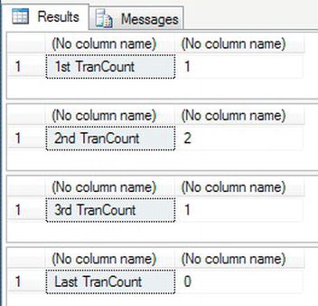
Figure 10-29. Showing the @@TRANCOUNT
![]() Note After the last
Note After the last COMMIT TRAN, @@TRANCOUNT is at 0. Any further instances of COMMIT TRAN or ROLLBACK TRAN will generate an error.
If in the code there is a ROLLBACK TRAN, then the data will immediately be rolled back no matter where you are within the nesting, and @@TRANCOUNT will be set to 0. Therefore, any further ROLLBACK TRAN or COMMIT TRAN instances will fail, so you do need to have error handling, which you look at in Chapter 14.
Try to avoid nesting transactions where possible, especially when one stored procedure calls another stored procedure within a transaction. It is not “wrong,” but it does require a great deal of care.
Now that updating data has been completed, the only area of data manipulation left is row deletion, which you will look at now.
Using More Than One Table
The SELECT, UPDATE, and DELETE statements have dealt with and covered only the retrieval of data from one table. However, it is possible to have more than one table used to retrieve data; but you must keep in mind that the more tables included in the query, the more detrimental the effect on the query's performance. However, it is sometimes faster to build one query that joins to more than one table rather than have several “one table” statements. If you are joining tables using an index, you will usually be fine as long as you do not have too many joins. A good rule of thumb is that as long as you are joining tables together using an index, then, until you start to have many joins, you should be okay. At all times, though, you should review your T-SQL. There is an aid called a query plan that you will see in Chapter 14. I would like to cover a bit more about more areas before I take you through a couple of basic query plans.
When you include subsequent tables, there must be a link of some sort between the two tables, known as a join. A join will take place between at least one column in one table and a column from the joining table. The columns involved in the join do not have to be in any key within the tables involved in the join. However, this is quite uncommon, and if you do find you are joining tables, then there is a high chance that a relationship exists between them, which would mean you do require a primary key and a foreign key. This was covered in Chapter 3.
It is possible that one of the columns on one side of the join is actually a concatenation of two or more columns. As long as the end result is one column, this is acceptable. Also, the two columns that are being joined do not have to have the same name, as long as they both have similar data types. For example, you can join a char with a varchar. What is not acceptable is that one side of the JOIN names a column and on the other side is a variable or literal that is really a filter that would be found in a WHERE statement. For example, you would not join on LastName equal to Dewson.
Joining two tables together can be relatively straightforward, but it can also become quite complicated. Let's consider the various types of joins:
INNER JOIN: The most basic join condition is a straight join between two tables, which is called anINNER JOIN. AnINNER JOINjoins the two tables, and where there is a join of data using the columns from each of the two tables, then the data are returned. For example, if there is a share in the shares table that has no price and you are joining the two tables on the share ID, then you would see output only where there is a share with a share price. You will see this in action in this chapter.OUTER JOIN: It is possible to return all the rows from one table where there is no join. This is known as anOUTER JOIN. Depending on which table you want the rows always to be returned from, this will be either aLEFT OUTER JOINor aRIGHT OUTER JOIN. Taking the shares example, you could use anOUTER JOINso that even when there is no share price, you can still list the share. This example will also be demonstrated later in this chapter.CROSS JOIN: The final type of join is the scariest and most dangerous join. If you wish for every row in one table to be joined with every row in the joining table, then you would use aCROSS JOIN. So if you had 10 rows in one table and 12 rows in the other table, you would see returned 120 rows of data (10×12). As you can imagine, this type of join just needs two small tables to produce even a large amount of output.
You might hear of one further join called a self join. This is using one of the foregoing techniques, but the join would be between the same table. This occurs when there is some reference identifier in a table that can be used to find another row in the same table, such as an ID called a parent ID.
Although not the most helpful of syntax demonstrated within the book, the syntax for joining two tables is as follows:
FROM tablea

 [FULL[INNER|OUTER|CROSS]] JOIN tableb

{ON tableb.column1 = tablea.column2 {AND|OR tableb.column...}}
The best way to look at the syntax is within a described example. I will use two tables to demonstrate the inner join in this example: ShareDetails.Shares and ShareDetails.SharePrices.
Joining two tables could not be simpler. All the columns in both tables are available to be returned through the query, so I can list the columns desired as normal. However, if there are two columns of the same name, they must be prefixed with the name, or the alias name, of the table from which the information is derived.
![]() Note It is recommended that whenever a join does take place, regardless of whether the column name is unique, all columns be prefixed with the table or alias name. This saves time if the query is expanded to include other tables, but it also clarifies exactly where the information is coming from.
Note It is recommended that whenever a join does take place, regardless of whether the column name is unique, all columns be prefixed with the table or alias name. This saves time if the query is expanded to include other tables, but it also clarifies exactly where the information is coming from.
TRY IT OUT: JOINING TWO TABLES
- The first join you will look at is the
INNER JOIN. This is where you have two tables, and you want to list all the values where there is a join. In this case, you want to list all the shares where there is a share price, and you want to see every share price for that share. Notice that you don't need to define the wordINNER. This is presumed if nothing else is specified. Also take note that, like columns, you have defined aliases for the table names. This makes prefixing columns easier. You are joining the two tables onShareId, as this is the linking column between the two tables. Enter the following code:SELECT s.ShareId, s.Description,sp.Price,sp.PriceDate
FROM ShareDetails.Shares s
JOIN ShareDetails.SharePrices sp ON sp.ShareId = s.ShareId
WHERE s.ShareId < 8
AND sp.PriceDate BETWEEN '1 Jan 2012' AND '3 Jan 2012' - Once you have executed the code, you should see the output that appears in Figure 10-30. There is no output for
ShareIds 4 and 6 as they have no share price between the dates in theWHERE.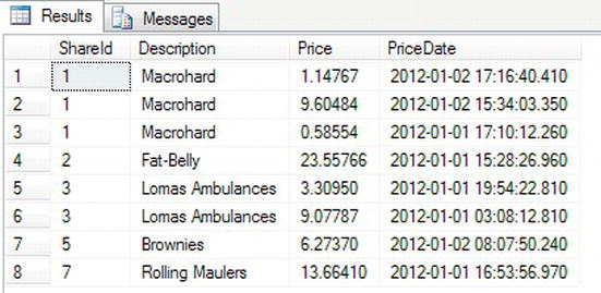
- You can take this a stage further and filter the rows to list only the share price row that matches the
CurrentPricein theShareDetails.Sharestable. This could be done by filtering the data on aWHEREstatement, and from a performance perspective it would be better, as neither of these columns are within an index and there could be a large number of rows forShareDetails.SharePricesfor each share as time goes on; but for this example, it demonstrates how to add a second column for the join.SELECT s.ShareDesc,sp.Price,sp.PriceDate
FROM ShareDetails.Shares s
JOIN ShareDetails.SharePrices sp ON sp.ShareId = s.ShareId
AND sp.Price < s.CurrentPrice
WHERE s.ShareId < 8
AND sp.PriceDate BETWEEN '1 Jan 2012' AND '3 Jan 2012' - Execute the preceding code, which returns the rows shown in Figure 10-31. As you can see, an
INNER JOINis very straightforward.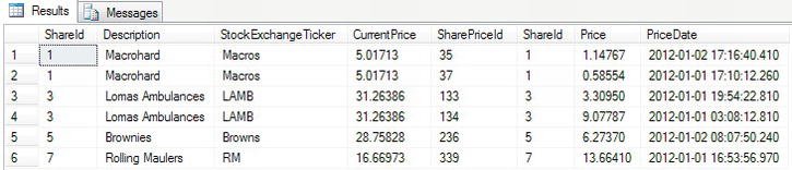
Figure 10-31. Inner join with multiple join columns
- You can combine more than one table using multiple joins and with a mixture of join types. In the next example, a request has been made where, for each customer, you would like to see all transactions that involved a share and what the current price is for the share. This involves joining the
CustomerDetails.Customerstable to theTransactionDetails.Transactionstable and then on to theShareDetails.Sharestable. From the customer table, you will retrieve the first and last name of the customer, the transaction ID and the transaction total amount from the transaction details table, and finally the share description and the current share price from the shares table. Enter the query details here, execute, and you should see the results, as shown in Figure 10-32.SELECT c.FirstName,c.LastName,t.TransactionId,t.Amount,
s.ShareId,s.Description, s.CurrentPrice
FROM CustomerDetails.Customers c
JOIN TransactionDetails.Transactions t ON t.CustomerId = c.CustomerId
JOIN ShareDetails.Shares s ON s.ShareId = t.RelatedShareId
WHERE s.ShareId < 8
AND sp.PriceDate BETWEEN '1 Jan 2012' AND '3 Jan 2012'
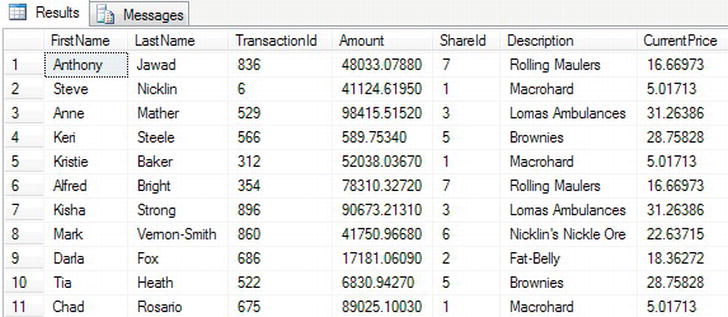
Figure 10-32. Multiple table join
Joining Tables with an Outer Join
The next join to look at is an OUTER JOIN—more specifically, a LEFT OUTER JOIN. In this instance, I want to return all the rows in the left table, regardless of whether there is any data in the right table. The left table in this case is the ShareDetails.Shares table, as it is the left named table of the two I am concerned with.
- Enter the following code:
SELECT s.ShareId,s.Description,sp.Price,sp.PriceDate

  FROM ShareDetails.Shares s

  LEFT OUTER JOIN ShareDetails.SharePrices sp ON sp.ShareId = s.ShareId

WHERE sp.PriceDate BETWEEN '1 Jan 2012' AND '3 Jan 2012' - Once you execute this code, you should see the missing shares from the previous example listed, as shown in Figure 10-33. Notice that where no data exist in the
ShareDetails.SharePricestable, the values are displayed asNULL.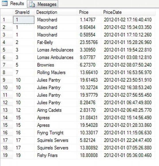
Figure 10-33. Left outer join
OUTER JOINSare a good tool when checking other queries. For example, the results in Figure 10-32 demonstrate that quite rightly, the bottom three shares should have been missing in the first example, as they did not meet the criteria. This may not be so obvious when there are large volumes of data, though. - Similar to the earlier multiple table join, you can mix in another type of join. In the code here, you will see the code from the
INNER JOINexample, but you also need to know where the share price is not being updated. This can be found by completing aLEFT OUTER JOINon theShareDetails.SharePricesbut listing only where theSharePricewasNULL. ANULLvalue from theLEFT OUTER JOINwill show that there is noSharePricerow, and therefore it is possible that the system is not collecting share prices. This is something that as a business that would need to be rectified so that you could provide the customers with an up-to-date valuation. Enter the following code:SELECT c.FirstName,c.LastName,t.TransactionId,t.Amount,
s.ShareId,s.Description, s.CurrentPrice,
sp.Price
FROM CustomerDetails.Customers c
JOIN TransactionDetails.Transactions t
ON t.CustomerId = c.CustomerId
JOIN ShareDetails.Shares s
ON s.ShareId = t.RelatedShareId
LEFT OUTER JOIN ShareDetails.SharePrices sp
ON sp.ShareId = s.ShareId
WHERE sp.Price IS NULL - Execute the code, and you see there are only 13 rows returned, as shown in Figure 10-34.
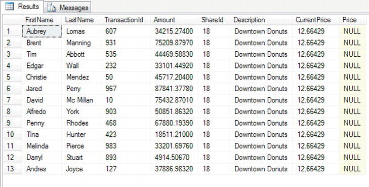
Figure 10-34. Multiple joins with a left outer showing a
NULLpriceThe next example is a
RIGHT OUTER JOIN. Here I expect the table on the right to return rows where there are no entries on the table in the left. In the example, such a scenario does not exist, as it would break referential integrity; however, I can swap the tables around, which shows the same results as the firstLEFT OUTER JOINexample. Take note that you don't have to alter the column order after theON, as it is the table definition that defines the left and right tables. - Enter the following code:
SELECT s.Description,sp.Price,sp.PriceDate

  FROM ShareDetails.SharePrices sp

  RIGHT OUTER JOIN ShareDetails.Shares s ON sp.ShareId = s.ShareId

WHERE sp.PriceDate BETWEEN '1 Jan 2012' and '3 Jan 2012' - Executing this code gives you the results shown in Figure 10-35.
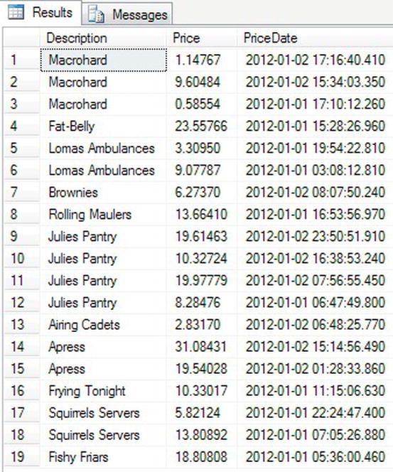
Figure 10-35. Right outer join
If you want a
LEFT OUTER JOINand aRIGHT OUTER JOINto be available at the same time, then you need to choose theFULL OUTER JOIN. This returns rows from both the left and right tables if there are no matching rows in the other table. So to clarify, if there is a row in the left table but no match in the right table, the row from the left table will be returned withNULLvalues in the columns from the right table, and vice versa. This time you are going to break referential integrity and insert a share price with no share. You will then delete the row to keep referential integrity intact. - Enter the following code:
SELECT s.Description,sp.Price,sp.PriceDate

  FROM ShareDetails.SharePrices sp

  FULL OUTER JOIN ShareDetails.Shares s ON sp.ShareId = s.ShareId

 WHERE s.Description IS NULL

OR sp.Price IS NULL - Once the preceding code has been executed, you will see the results that appear in Figure 10-36. Notice that you have a row from the
ShareDetails.Sharestable when there is no share price, and vice versa.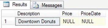
Figure 10-36. Full outer join
Working with a CROSS JOIN
The final demonstration is with a CROSS JOIN. This is a Cartesian join between the ShareDetails.Shares and ShareDetails.SharePrices tables. A CROSS JOIN cannot have any filtering on it; therefore, it cannot include a WHERE statement. As you are joining every row with every row, there is no need to provide an ON statement, because there is no specific row-on-row join. Due to the vast amount of data, to make it easier for you to scroll through, I have put a TOP 4000 clause in the query and ordered the results by ShareId and SharePriceId. This will then allow you to see that for every SharePrice there are 1,000 share rows.
- Enter the following code:
SELECT TOP 100 s.ShareId,sp.SharePriceId,

s.Description,sp.Price,sp.PriceDate

  FROM ShareDetails.SharePrices sp

  CROSS JOIN ShareDetails.Shares s

WHERE sp.PriceDate BETWEEN '1 Jan 2012' and '3 Jan 2012'

ORDER BY ShareId,SharePriceId - The preceding code, when executed, generates a large amount of output. Figure 10-37 shows only a snippet of the output.

Figure 10-37. Cross join
It will be rare that you write a cross join, and, given the dangerous nature of these joins, you should restrict the number of rows returned where possible. You should also ensure testing of any cross join is completed on a test database prior to running against a production database instance.
Summary
This chapter has taken a look at how to retrieve data on a set of tables in the simplest form. Later in the book, you will return to retrieving data with more complex language as well as working with data from more than one table within the single query. You should also be comfortable with getting information from tables using different searching, filtering, and ordering criteria.
Updating data can go wrong, and does, especially when you are working in a live environment and you wish to update data that is in flux. In such a scenario, getting the correct rows of information to update and then actually updating them is akin to a fine art.
Therefore, surrounding any of your work with a transaction will prevent any costly and potentially irretrievable mistakes from taking place, so always surround data modifications or deletions with a transaction. With data inserts, it is not quite so critical that you surround your work with a transaction, although it is recommended. For example, if you are inserting data within a test environment and the data insertion is easily removed if you have part of the insertion wrong, then perhaps it's not overly critical to use a transaction; although to be safe, really and truly, I still recommend that you use a transaction.
Updating columns within a table is very straightforward. As long as the data type defined for the column to update is the same as, or is compatible with, the data type of the column, variable, or static value that is being used to update this column, then you will have no problem. For example, you can update a varchar column with char data type values. However, it is not possible to update an integer column with a varchar value that has a noninteger value without converting the varchar value to an integer. But don't be fooled, you can update a varchar with an integer or numeric data type.
Finally you saw how to join two or more tables and the different methods you can use to achieve the desired results. Joining tables will become a staple of your coding diet, and, although only SELECT statements were demonstrated with joins, you can use the same techniques for DELETE and UPDATE. For these statements, you would use the joins to either create the ability to filter the data or return values for updating the data. You will see more about joins throughout the book.
So where can you go from here? The next chapter will look at views of data.