C H A P T E R 14
Advanced T-SQL and Debugging
By now, you really are becoming proficient in SQL Server 2012 and writing code to work with the data and the objects within the database. Already you have seen some T-SQL code and encountered some scenarios that have advanced your skills as a T-SQL developer. You can now look at more advanced areas of T-SQL programming to round out your knowledge and really get you going with queries that do more than the basics.
This chapter will cover the occasions when you need a query within a query, known as a subquery. This is ideal for producing a list of values to search for, or for producing a value from another table to set a column or a variable with. It is also possible to create a transient table of data to use within a query, known as a common table expression. You will look at both subqueries and common table expressions in this chapter.
From there, you will explore how to take a set of data and pivot the results, just as you can do within Excel. You will also take a look at different types of ranking functions, where you can take your set of data and attach rankings to rows or groups of rows of data.
Finally, you will see how to deal with varchar(max) and varbinary(max) data types when loading large text, images, movies, and so on.
Sequences Instead of IDENTITY
In Chapter 5, you were introduced to IDENTITY columns, in which an identity value would be automatically generated when there was an attempt to add a new row. As I mentioned, gaps could be created either when a single- or multiple-row insertion failed or was rolled back as part of a transaction. IDENTITY-defined columns are ideal for small, low-frequency row insertions, but there is a small performance overhead each time a value is created. It has been requested for some time from developers that Microsoft look at this problem and find a way to improve performance, and so from this problem, Microsoft has developed sequences.
The first benefit of sequences is that it is possible for SQL Server not only to retrieve the next value one at a time from the underlying sequence table (like IDENTITY), but also to cache a range of numbers in memory for faster access and retrieval. A cached set of numbers will work faster than using the IDENTITY property, which is generated with each insertion.
You can also define a sequence so that the sequence can loop around when a maximum value is reached. This allows you to reuse numbers.
It is also possible to retrieve the next sequence value and place it into a local variable before the row is inserted. This will give you the flexibility of knowing the “identity” column value for any child tables’ insertions. With IDENTITY, you can retrieve the value assigned to a row only after the row is inserted. By having the ability to assign the value to a variable with sequence, you can avoid gaps through insertions failing by reusing the value if, for example, a rollback occurs. Gaps will still form, though, if the server is rebooted or the SQL Server Windows service stopped, so using a local variable is not a complete solution to the gapping issue.
Sequences can deal with generating a value for multiple tables and potentially different columns all from the single sequencing object, unlike the IDENTITY keyword, which is bound to one column in one table. The ability to split sequencing across multiple tables allows you to keep the sequence of data intact if, for example, you have a table holding incoming records but two tables for processed data—one for accepted records and one for rejected records. By inspecting the sequence column value on both these tables, you would be able to see the order in which the rows had been processed.
![]() Caution If you use sequences within a transaction and the transaction is rolled back, then the sequence is not rolled back and the values retrieved will look as if they have been used.
Caution If you use sequences within a transaction and the transaction is rolled back, then the sequence is not rolled back and the values retrieved will look as if they have been used.
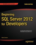
Using sequences, you can assign a value to a column programmatically. This functionality removes the problems that can occur when using IDENTITY because IDENTITY column values are awkward to alter within a column after they are assigned. When completing a bulk insertion or even modifying the value within a column, an incorrectly inserted value can be modified when using sequences, as you will see in the ALTER SEQUENCE section of the exercise that follows. The downside, however, is that developers have to be aware that a column is logically linked to a sequence and use the sequence functionality rather than enter values manually. You can apply a sequence as a default value to the relevant column, as shown in Figure 14-1. This will still allow you to insert the sequence value like IDENTITY. However, when I use a sequence in the exercises in this section, I will not use it as a default value so that you can see explicitly what is happening.
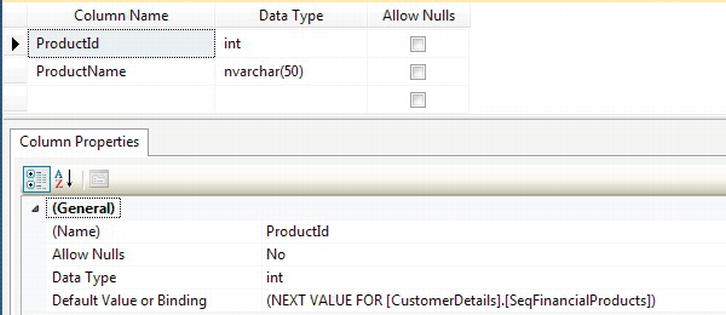
Figure 14-1. Applying a sequence as a default value for a column
Let’s take a look at how to create a sequence, including the syntax and the options that are available.
Creating a SEQUENCE
A sequence is held in its own object with a separate node under Programmability within SSMS. This helps to logically break the link between a sequence and its assignment to a specific table. Creating a sequence is more in tune with programming functions, such as a stored procedure, as you will see when looking at the syntax.
The syntax for the SEQUENCE object is very basic, with a number of options that can be attached to the sequence creation. The syntax is as follows:
CREATE SEQUENCE [schema_name . ] sequence_name

    [ AS [ built_in_integer_type | user-defined_integer_type ] ]

    [ START WITH <constant> ]

    [ INCREMENT BY <constant> ]

    [ { MINVALUE [ <constant> ] } | { NO MINVALUE } ]

    [ { MAXVALUE [ <constant> ] } | { NO MAXVALUE } ]

    [ CYCLE | { NO CYCLE } ]

    [ { CACHE [ <constant> ] } | { NO CACHE } ]
The CREATE SEQUENCE has a number of options; the only mandatory option is the sequence_name. The options are as follows:
schema_name: The schema that the sequence belongs tosequence_name: The name you want to call the sequenceAS: Although optional, I would recommend defining the data type to avoid confusion. If not defined, though, the data type will bebigint. Valid base data types aretinyint,smallint,int,bigint,decimal, andnumeric. Any user-defined type based on one of these base data types could also be assigned.START WITH: The number the sequence starts with; 1 is the default.INCREMENT BY: Each time a sequence number is requested, this defines the increment from the previous number. This can be a negative (for descending numbers) or positive, and the default increment is 1.MINVALUE value|NO MINVALUE: This is used in conjunction with theCYCLEoption. This will define the minimum value if the sequence numbers exceed theMAXVALUEif defined, and theCYCLEoption is defined. The default is the minimum value for the data range for the data type of the sequence.MAXVALUE value|NO MAXVALUE: This is used to define the maximum value of the sequence. The default is the maximum value for the data type. If the sequence reaches the maximum value, the next request for a number will generate an error if you haveNOCYCLEdefined or will put the sequence to theMINVALUEifCYCLEis defined.CYCLE|NO CYCLE: When the maximum value for a sequence is reached, it can generate an error ifNO CYCLEis defined, or will set the sequence toMINVALUEifCYCLEis defined.CACHE|NO CACHE: Every time you want the next number in the sequence, SQL Server will perform disk I/O to retrieve the value when usingNO CACHE. It is possible to cache a range of numbers in memory so that you retrieve the next value from memory, which is a great deal faster. SQL Server will generate the numbers and write the last number to disk, holding the numbers in memory for use. To achieve this, you would create the sequence with theCACHEoption, which is the default. The downside toCACHEis that if you need to restart the server or the SQL Server windows process, then that range of numbers in memory will be lost and a gap will exist. If that is not an issue and you are inserting a large number of rows, thenCACHEwould be a good choice.
Once a sequence is created, you then retrieve the next value using the following:
NEXT VALUE FOR [schema_name.]sequence_name
Now that you know what a sequence is and the options available, it is time to build and alter a sequence. A sequence will be built for the CustomerDetails.FinancialProducts table that already has data within it. You will see valid insertions to the table, and then you will see what happens when a maximum is reached and how to progress from that point.
TRY IT OUT: BUILDING AND USING A SEQUENCE
- First of all, it is useful to know what number the sequence will start at based on the maximum value of
ProductIds within theCustomerDetails.FinancialProductstable.SELECT MAX(ProductId) + 1
FROM CustomerDetails.FinancialProducts - Next, the sequence is created within the
CustomerDetailsschema with a unique name. The return value will be an integer and will start at 42, as product ID 41 is my last financial product ID. For the moment, I am setting a max value of 44 and that each sequence will be retrieved one at a time, no caching. Execute the following code.CREATE SEQUENCE CustomerDetails.SeqFinancialProducts
AS int
START WITH 42
MAXVALUE 44
NO CACHE Note You cannot use a local variable to define any values for options. It has to be a constant.
 - You should then see the sequence under the Programmability node within Object Explorer for SQL Server, as shown in Figure 14-2.
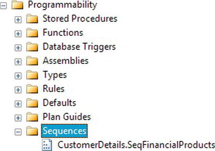
Figure 14-2. The new sequence created and showing in Object Explorer
- You can now test the sequence by inserting three rows of data. This will keep the sequence number within the bounds of the max value. When you execute the code, all three rows should insert successfully.
INSERT CustomerDetails.FinancialProducts(ProductId, ProductName)

    VALUES (NEXT VALUE FOR CustomerDetails.SeqFinancialProducts,

            'Life Insurance') ,

        (NEXT VALUE FOR CustomerDetails.SeqFinancialProducts,

            'Unit Trusts'),

        (NEXT VALUE FOR CustomerDetails.SeqFinancialProducts,

'Investment Trusts') - The next insertion will fail. Enter the following code for the next insertion.
INSERT CustomerDetails.FinancialProducts(ProductId, ProductName)

    VALUES (NEXT VALUE FOR CustomerDetails.SeqFinancialProducts,

'Repurchase Agreements') - When you execute the code, you will see an error, as shown here:
Msg 11728, Level 16, State 1, Line 1

The sequence object 'SeqFinancialProducts' has reached its

minimum or maximum value. Restart the sequence object to allow

new values to be generated.
At this point, all further insertions will fail, which may be a valid scenario for your system; however, if it is not, then you need to build your sequence with an alternative strategy in mind.
In the next section, you will see how to alter the sequence so that insertions can be successfully completed going forward. This is achieved via the ALTER SEQUENCE command.
Before you dive into altering the sequence, you need to know what the syntax is. It is very similar to the CREATE SEQUENCE as it has the same options; however, there is a further option called RESTART. RESTART on its own, which is the default, would reseed the sequence to the lowest value for the data type, which would be -2,147,483,648 for the int data type. To restart with a specific value, you add WITH and a constant value. You will see this in the following exercise. The syntax follows, and then the exercise will use this syntax to alter the sequence:
ALTER SEQUENCE [schema_name. ] sequence_name

    [ RESTART [ WITH <constant> ] ]
- The first example will demonstrate cycling the sequence only. This will cause the sequence to loop around to the beginning, and as there is no
RESTARToption you will see the data type’s minimum value added for the new row.ALTER SEQUENCE CustomerDetails.SeqFinancialProducts
CYCLE - Insert the row of data that in the
CREATE SEQUENCEexample failed as the maximum was reached. When you execute the code this time, it will succeed.INSERT CustomerDetails.FinancialProducts(ProductId, ProductName)
VALUES (NEXT VALUE FOR CustomerDetails.SeqFinancialProducts, 'Repurchase
Agreements') - You can check the value given to the row from the sequence via the following code.
SELECT ProductId,ProductName

FROM CustomerDetails.FinancialProducts

ORDER BY ProductId - When you execute the code, you will see the row as shown in Figure 14-3.
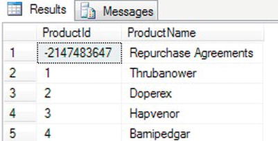
Figure 14-3. New row inserted with the minimum value
- As this was generated in error, you could modify the
ProductIdwith anUPDATE; however, for this example, let’s delete the row so it can be inserted correctly. - You now need to alter the sequence to indicate the restart value of 1. You will also need to
CYCLEthe sequence.ALTER SEQUENCE CustomerDetails.SeqFinancialProducts
CYCLE
RESTART WITH 1 - It is now possible to insert the row with the correct sequence value of 1 and then inspect the table to see if the
ProductIdis 1.INSERT CustomerDetails.FinancialProducts(ProductId, ProductName)
VALUES (NEXT VALUE FOR CustomerDetails.SeqFinancialProducts,
'Repurchase Agreements')
SELECT ProductId,ProductName
FROM CustomerDetails.FinancialProducts
ORDER BY ProductId - This time the correct sequence has been generated, but notice in Figure 14-4 that you now have two rows with a
ProductIdof 1, which is what was desired with the alter sequence in step 6.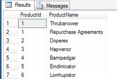
Figure 14-4. Row now inserted with the restarted value
If you wanted the sequence to carry on, then you would have, in step 6, set a new maximum value and set the RESTART WITH value to the max value in the ProductId column and not CYCLEd the sequence. You can delete one of the ProductId ones by executing the following code. I have deleted one of the rows.
DELETE TOP (1) FROM CustomerDetails.FinancialProducts where ProductId = 1
Subqueries
A subquery is a query embedded within another query or statement and can be used anywhere an expression is allowed. It can be used to check or set a value of a variable or column, or used to test whether a row of data exists in a WHERE clause.T-SQL code
Using Subqueries
Sometimes, you may want to set a column value based on data from another query. One example you have is the ShareDetails.Shares table. .Imagine you have a column defined for MaximumSharePrice that holds the highest price the share price had reached for that year. Rather than doing a test every time the share price moved, you could use the MAX function to get the highest share price, put that value into a variable, and then set the column via that variable. Without the use of a subquery, with the exception of the ALTER TABLE, the code would be similar to that defined here:
ALTER TABLE ShareDetails.Shares

ADD MaximumSharePrice money

GO

DECLARE @MaxPrice money

SELECT @MaxPrice = MAX(Price)

    FROM ShareDetails.SharePrices

  WHERE ShareId = 1

SELECT @MaxPrice

UPDATE ShareDetails.Shares

SET MaximumSharePrice = @MaxPrice

WHERE ShareId = 1
In the preceding code, if you wanted to work with more than one share, you would need to implement a loop and process each share one at a time. However, you could also perform a subquery, which implements the same functionality as shown in the code that follows. The subquery still finds the maximum price for a given share and sets the column. Notice that this time you can update all shares with one statement. The subquery joins with the main query via a WHERE clause so that as each share is dealt with, the subquery can take that ShareId and still get the maximum value. If you want to run the following code, then you still need the ALTER TABLE statement used previously, even if you did not run the preceding code.
![]() Note This type of subquery is called a correlated subquery.
Note This type of subquery is called a correlated subquery.
SELECT ShareId,MaximumSharePrice

FROM ShareDetails.Shares

UPDATE ShareDetails.Shares

SET MaximumSharePrice =

    (SELECT MAX(Price)

       FROM ShareDetails.SharePrices sp

      WHERE sp.ShareId = s.ShareId)

FROM ShareDetails.Shares s

SELECT ShareId,MaximumSharePrice
FROM ShareDetails.Shares
You also came across a subquery way back in Chapter 7 when you were testing whether a backup had successfully completed. The code is replicated here, with the subquery section highlighted in bold. In this instance, instead of setting a value in a column, you are looking for a value to be used as part of a filtering criterion. Recall from Chapter 7 that you know the last backup will have the greatest backup_set_id. You use the subquery to find this value (as there is no system function or variable that can return this at the time of creating the backup). Once you have this value, you can use it to reinterrogate the same table, filtering out everything but the last row for the backup just created.
![]() Note Don’t forget that for the
Note Don’t forget that for the FROM DISK option, you will have a different file name than the one in the following code.
declare @backupSetId as int

select @backupSetId = position

from msdb..backupset

where database_name=N'ApressFinancial'

and backup_set_id=(select max(backup_set_id)

                    from msdb..backupset

                   where database_name=N'ApressFinancial')

if @backupSetId is null

begin

    raiserror(N'Verify failed. Backup information for

    database ''ApressFinancial'' not found.', 16, 1)

end

RESTORE VERIFYONLY

FROM DISK = N'C:Program FilesMicrosoft SQL Server

MSSQL11.APRESS_DEV1MSSQLBackupApressFinancial.bak'

WITH FILE = @backupSetId,

NOUNLOAD,

NOREWIND

GO
In both of these cases, you are returning a single value within the subquery, but this need not always be the case. You can also return more than one value. One value must be returned when you are trying to set a value. This is because you are using an equals (=) sign. It is possible in a WHERE clause to look for a number of values using the IN clause.
IN
If you want to look for a number of values in your WHERE clause, such as a list of values from the ShareDetails.Shares table where the ShareId is 1, 11, or 15, then you can use an IN clause. The code to complete this example would be as follows:
SELECT *

  FROM ShareDetails.Shares

 WHERE ShareId IN (1,11,15)
Using a subquery, it would be possible to replace these numbers with the results from the subquery. The preceding query could also be written using the code that follows. This example shows how it is possible to combine a subquery and an aggregation to produce the list of ShareIds that form the IN:
SELECT *

  FROM ShareDetails.Shares

 WHERE ShareId IN (SELECT ShareId

                     FROM ShareDetails.Shares

                    WHERE CurrentPrice > (SELECT MIN(CurrentPrice)

                                            FROM ShareDetails.Shares)

                      AND CurrentPrice < (SELECT MAX(CurrentPrice) / 3

                                            FROM ShareDetails.Shares))
![]() Note If a query starts becoming very complex, you may find that it starts performing badly. This book doesn’t look at the performance of queries, although it has discussed indexes and how they can help your query perform better. Always take a step back and think, “Would this work better as two queries where the first query creates a subset of data?” Writing a very complex query that processes all the data in one pass may not always be the best answer. Consider also that a complex query can be difficult to figure out should you need to revise later.
Note If a query starts becoming very complex, you may find that it starts performing badly. This book doesn’t look at the performance of queries, although it has discussed indexes and how they can help your query perform better. Always take a step back and think, “Would this work better as two queries where the first query creates a subset of data?” Writing a very complex query that processes all the data in one pass may not always be the best answer. Consider also that a complex query can be difficult to figure out should you need to revise later.
Both of these examples replace what would require a number of OR clauses within the WHERE filter, such as you see in this code:
SELECT *

  FROM ShareDetails.Shares

 WHERE ShareId = 1

   OR ShareId = 11

   OR ShareId = 15
These are just three different ways a subquery can work. The fourth way involves using a subquery to check whether a row of data exists, which you will look at next.
EXISTS
EXISTS is a clause that is very similar to IN, in that it tests a column value against a subset of data from a subquery. The difference is that EXISTS uses a join to join values from a column to a column within the subquery, as opposed to IN, which compares against a comma-delimited set of values and requires no join.
Over time, your ShareDetails.Shares and ShareDetails.SharePrice tables will grow to quite large sizes. If you wanted to shrink them, you could use cascading deletes so that when you delete from the ShareDetails.Shares table, you would also delete all the SharePrice records. But how would you know which shares to delete? One way would be to see what shares are still held within your TransactionDetails.Transactions table. You would do this via EXISTS, but instead of looking for ShareIds that exist, you would use NOT EXISTS.
At present, you have no shares listed within the TransactionDetails.Transactions table, so you would see all of the ShareDetails.Shares listed. You can make life easier with EXISTS by giving tables an alias, but you also have to use the WHERE statement to make the join between the tables. However, you aren’t really joining the tables as such; a better way of looking at it is to say you are filtering rows from the subquery table.
The final point to note is that you can return whatever you want after the SELECT statement in the subquery, but it should be only one column or a value; it cannot be more than this. The subquery can be in the columns returned and the single value returned, displayed along with the other columns. However, if subquery is in the WHERE condition, then the value cannot be displayed.
![]() Note When using
Note When using EXISTS, it is most common in SQL Server to use * rather than a constant like 1, as it simply returns a true or false setting.
The following code shows EXISTS in action prefixed with a NOT:
SELECT *

  FROM ShareDetails.Shares s

 WHERE NOT EXISTS (SELECT *

                     FROM TransactionDetails.Transactions t

                    WHERE t.RelatedShareId = s.ShareId)
![]() Note Both
Note Both EXISTS and IN can be prefixed with NOT.
Tidying Up the Loose End
You have a loose end from a previous chapter that you need to tidy up. In Chapter 12, you built a scalar function to calculate interest between two dates using a rate. It was called TransactionDetails.fn_IntCalc. When I demonstrated this, you had to pass in the specific information; however, by using a subquery, it is possible to use this function to calculate interest for customers based on their transactions. The following “Try it Out” exercise shows you how to invoke the function with a subquery result as one of the arguments. The subquery computes the “to date” for each transaction returned by the outermost SELECT statement.
TRY IT OUT: USING A SCALAR FUNCTION WITH SUBQUERIES
- In the first part of the query, you are returning some data from the
TransactionDetails.Transactionstable:SELECT t1.TransactionId, t1.DateEntered,t1.Amount, - The second part of the query is where it is necessary to compute the “to date” for calculating the interest, as
DateEnteredwill be used as the “from date.” To do this, it is necessary to find the next transaction in theTransactionDetails.Transactionstable. To do that, you need to find the minimumDateEntered—using the minimum function—where that minimumDateEnteredis greater than that for the transaction you are on in the main query. However, you also need to ensure you are doing this for the same customer as theSELECTused previously. You need to make a join from the main table to the subquery joining on the customer ID. Without this, you could be selecting any minimum date entered from any customer.SELECT MIN(DateEntered)
FROM TransactionDetails.Transactions t2
WHERE t2.CustomerId = t1.CustomerId
AND t2.DateEntered> t1.DateEntered) as 'To Date', - Finally, you can put the same query into the call to the interest calculation function. The final part is where you are just looking for the transactions for customer ID 1. The following is the entire query. The outer query invokes the function. One of the arguments to the function is the result of the subquery that computes each transaction’s “to date.”
SELECT t1.TransactionId, t1.DateEntered,t1.Amount,

TransactionDetails.fn_IntCalc(3,t1.Amount,t1.DateEntered,

(SELECT MIN(DateEntered)

FROM TransactionDetails.Transactions t2

WHERE t2.CustomerId = t1.CustomerId

AND t2.DateEntered> t1.DateEntered)) AS 'Interest Earned'

FROM TransactionDetails.Transactions t1

WHERE CustomerId = 1 - Once you have the code together, you can then execute the query, which should produce output as shown in Figure 14-5.
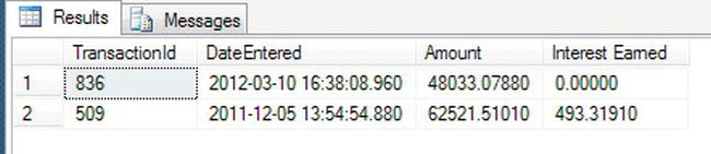
Figure 14-5. Using a subquery to call a function
The APPLY Operator
It is possible to return a table as the data type from a function. The table data type can hold multiple columns and multiple rows of data as you would expect, and this is one of the main ways it differs from other data types, such as varchar, int, and so on. Returning a table of data from a function gives the code invoking the function the flexibility to work with returned data as if the table permanently existed or was built as a temporary table.
To supply extensibility to this type of function, SQL Server provides you with an operator called APPLY, which works with a table-valued function and joins data from the calling table(s) to the data returned from the function. The function will sit on the right-hand side of the query expression, and, through the use of APPLY, can return data as if you had a RIGHT OUTER JOIN or a LEFT OUTER JOIN on a “permanent” table. Before you see an example, you need to be aware that there are two types of APPLY: a CROSS APPLY and an OUTER APPLY.
CROSS APPLY: Returns only the rows that are contained within the outer table where the row produces a result set from the table-valued functionOUTER APPLY: Returns the rows from the outer table and the table-valued function regardless of whether a join exists; this is similar to anOUTER JOIN, which you saw in Chapter 10. If no row exists in the table-valued function, then you will see aNULLin the columns from that function.
CROSS APPLY
In your example, you will build a table-valued function that accepts a CustomerId as an input parameter and returns a table of TransactionDetails.Transactions rows.
TRY IT OUT: TABLE FUNCTION AND CROSS APPLY
- Similar to what you did in Chapter 12, you will create a function with input and output parameters, followed by a query detailing the data to return. The difference in this example is that a table of data will be returned rather than a single value. Therefore, you need to name the table using a local variable followed by the
TABLEclause. You then need to define the table layout for every column and data type. Enter the following code, and then execute it to create the function.CREATE FUNCTION TransactionDetails.ReturnTransactions
(@CustId bigint) RETURNS @Trans TABLE
(TransactionId bigint,
CustomerId bigint,
TransactionDescription nvarchar(30),
DateEntered datetime,
Amount money)
AS
BEGIN
INSERT INTO @Trans
SELECT t.TransactionId, t.CustomerId, tt.Description,
t.DateEntered, t.Amount
FROM TransactionDetails.Transactions t
JOIN TransactionDetails.TransactionTypes tt ON
tt.TransactionTypeId = t.TransactionType
WHERE CustomerId = @CustId
RETURN
END
GO - Now that you have the table-valued function built, you can call it and use
CROSS APPLYto return only theCustomerDetails.Customersrows where there is a customer number within the table from the table-valued function. To clarify what is happening, for every row found in theSELECTcommand that is retrieving customers from theCustomerDetails.Customerstable, theCustomerIdis passed to the function created in the first step, the function returns a table of data that has a name alias ofTrans, and the table of data is then joined using theCROSS APPLYclause to theCustomerDetails.Customerstable to give the results. The following code demonstrates this:SELECT c. FirstName, LastName,
Trans.TransactionId,TransactionDescription,
DateEntered,Amount
FROM CustomerDetails.Customers AS c
CROSS APPLY
TransactionDetails.ReturnTransactions(c.CustomerId)
AS Trans - The results from the preceding code are shown in Figure 14-6, where you can see that only rows from the
CustomerDetails.Customerstable are displayed where there is a corresponding row in theTransactionDetails.Transactionstable.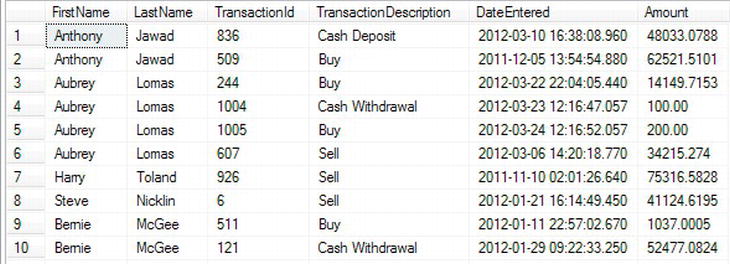
Figure 14-6. Partial results of the
CROSS APPLYfrom a table-valued function
OUTER APPLY
As mentioned previously, OUTER APPLY is very much like a RIGHT OUTER JOIN on a table, but you need to use OUTER APPLY when working with a table-valued function.
For your example, you can still use the function you built for the CROSS APPLY. With the code that follows, you are expecting those customers that have no rows returned from the table-valued function to be listed with NULL values.
TRY IT OUT: TABLE FUNCTION AND OUTER APPLY
- Enter the following code, which will perform an
OUTER APPLYon the user-defined function created in the previous example.SELECT c. FirstName, LastName,
Trans.TransactionId,TransactionDescription,
DateEntered,Amount
FROM CustomerDetails.Customers AS c
OUTER APPLY
TransactionDetails.ReturnTransactions(c.CustomerId)
AS Trans - When this is executed, you will see the output shown in Figure 14-7. Only part of the output is shown.
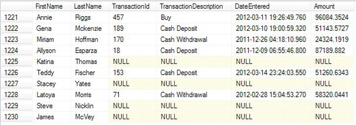
Figure 14-7.
OUTER APPLYfrom a table-valued function
Common Table Expressions
A common table expression (CTE) is a bit like a temporary table. It’s transient, lasting only as long as the query requires it. Temporary tables are available for use during the lifetime of the session of the query running the code or until they are explicitly dropped. The creation and use of temporary tables are a two- or three-part process: table creation, population, and use. A CTE is built in the same code line as the SELECT, INSERT, UPDATE, or DELETE statements that use it.
Using Common Table Expressions
As mentioned a CTE lasts only as long as the query that uses it. If you need a set of data to exist for this amount of time only, then a CTE can be better in performance terms than a temporary table. In Chapter 13, you had a look at temporary tables by defining a table in code and prefixing the name with a hash mark (#). The best way to understand a CTE is to demonstrate an example with some code.
The first example code will build a temporary table and then use this within a query. The second example will demonstrate how to complete the same task but by using a CTE and will show how simple the code can be. First of all, it is necessary to download the Microsoft sample database AdventureWorks and install it on your system. The code and installation instructions can be found on the CodePlex site, www.codeplex.com. I am using this database as it has a good set of mixed and related data. This is also possible to achieve within the Red Gate SQL Data Generator software but takes time, and as a developer, unless there is good reason to reinvent the wheel, don’t.
Within the AdventureWorks sample database, there are a number of products held in the Production.Product table. For this example, let’s say you want to know the maximum list price of stock you’re holding over all the product categories. Using a temporary table, this would be a two-part process, as follows:
USE AdventureWorks2008R2

GO

SELECT p.ProductSubcategoryID, s.Name,SUM(ListPrice) AS ListPrice

  INTO #Temp1

  FROM Production.Product p

  JOIN Production.ProductSubcategory s ON s.ProductSubcategoryID =

    p.ProductSubcategoryID

 WHERE p.ProductSubcategoryID IS NOT NULL

 GROUP BY p.ProductSubcategoryID, s.Name


SELECT ProductSubcategoryID,Name,MAX(ListPrice)

  FROM #Temp1

  GROUP BY ProductSubcategoryID, Name

HAVING MAX(ListPrice) = (SELECT MAX(ListPrice) FROM #Temp1)


DROP TABLE #Temp1
However, with CTEs, this becomes a bit simpler and more efficient. In the preceding code snippet, I have created a temporary table. This table has no index on it, and therefore SQL Server will complete a table scan operation on it when executing the second part. In contrast, the upcoming code snippet uses the raw AdventureWorks tables. There is no creation of a temporary table, which would have used up processing time, and also existing indexes could be used in building up the query, rather than a table scan.
The CTE is built up using the WITH keyword, which defines the name of the CTE you’ll be returning—in this case, ProdList—and the columns contained within it. The columns returned within the CTE will take the data types placed into it from the SELECT statement within the parentheses. Of course, the number of columns within the CTE has to be the same as the table defined within the brackets. This table is built up, returned, and passed immediately into the following SELECT statement outside of the WITH block, where the rows of data can then be processed as required. Therefore, the rows returned between the brackets could be seen as a temporary table that is used by the statement outside of the brackets.
WITH ProdList (ProductSubcategoryID,Name,ListPrice) AS

(

SELECT p.ProductSubcategoryID, s.Name,SUM(ListPrice) AS ListPrice

  FROM Production.Product p

  JOIN Production.ProductSubcategory s ON s.ProductSubcategoryID =

    p.ProductSubcategoryID
  WHERE p.ProductSubcategoryID IS NOT NULL

  GROUP BY p.ProductSubcategoryID, s.Name

)

SELECT ProductSubcategoryID,Name,MAX(ListPrice)

  FROM ProdList

  GROUP BY ProductSubcategoryID, Name

  HAVING MAX(ListPrice) = (SELECT MAX(ListPrice) FROM ProdList)
When the code is executed, the results should resemble the output shown in Figure 14-8.
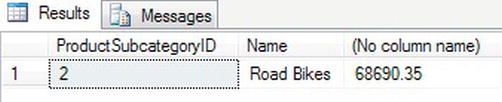
Figure 14-8. CTE output
Recursive CTE
A recursive CTE is where an initial CTE is built and then the results from that are called recursively in a UNION statement, returning subsets of data until all the data are returned. This gives you the ability to create data in a hierarchical fashion, as you will see in the next example. An example of a recursive CTE would be where you have a row of data that is linked to another row of data, such as a table that holds employee details (which is the example you will build shortly). You would have the owner at the top, followed by the CEO, the board of directors, the people who report to the board, and all the way down to the graduate intern. A recursive CTE would look at the results at each level of the organization.
The basis of building a recursive CTE is to build your initial query just as you saw earlier, but then append to that a UNION ALL statement with a join on the cte_name. This works so that in the “normal” CTE, data are created and built with the cte_name, which can then be referenced within the CTE from the UNION ALL. The syntax that you can see here demonstrates how this looks in its simplest form:
WITH cte_name ( column_name [,...n] )

AS

(

CTE_query_definition

UNION ALL

CTE_query_definition with a join on cte_name

)
As with all UNION statements, the number of columns must be the same in all queries that make up the recursive CTE. The data types must also match up.
![]() Caution Care must be taken when creating a recursive CTE. It is possible to create a recursive CTE that goes into an infinite loop. While testing the recursive CTE, you can use the
Caution Care must be taken when creating a recursive CTE. It is possible to create a recursive CTE that goes into an infinite loop. While testing the recursive CTE, you can use the MAXRECURSION option, as you will see in the next example.
The following example demonstrates a recursive query that will list every employee, their job titles, and the names of their managers. This example has a number of complexities, which are needed to get that reporting functionality to work because of the design of the AdventureWorks2008R2 schema. However, in many ways, this complexity is a positive development, because you should be becoming very competent in understanding the complexities required to use SQL Server. Where the AdventureWorks2008R2 database becomes quite complex is in how it structures the hierarchy of employees and managers within the organization. To get the hierarchy, you need to use a system function, GetAncestor. The GetAncestor function works alongside the hierarchyid data type to retrieve the parent node of a hierarchical set of data. You’ll use GetAncestor in the following example to return the parent—in this case, the manager—of the employee within the organization that you are inspecting. GetAncestor has a positive number as the input parameter that determines how many nodes to move within the hierarchy. A parameter of 1 would mean that you want to return the parent of the hierarchy identifier you are inspecting; a parameter value of 2 would be the grandparent, and so on.
Each employee in the HumanResources.Employee table has a hierarchyid data type in a column called OrganizationNode. The example can use the data in OrganizationNode with the GetAncestor function as I have just described. The GetAncestor function will be passed with the parameter value of 1, indicating that we want the parent of the employee, and by combining this returned value with a JOIN clause, the example can perform a join to find that parent row. This then allows you to use this knowledge to build your recursive CTE to build up the organizational hierarchy.
USE AdventureWorks2008R2

GO

WITH [EMP_cte]([BusinessEntityID], [OrganizationNode], [FirstName],

[LastName], [RecursionLevel]) -- CTE name and columns

AS (

SELECT e.[BusinessEntityID], e.[OrganizationNode], p.[FirstName],

p.[LastName], 0

FROM [HumanResources].[Employee] e

INNER JOIN [Person].[Person] p

ON p.[BusinessEntityID] = e.[BusinessEntityID]

WHERE e.[BusinessEntityID] = 2

UNION ALL

SELECT e.[BusinessEntityID], e.[OrganizationNode], p.[FirstName],

p.[LastName], [RecursionLevel] + 1 -- Join recursive member to anchor

FROM [HumanResources].[Employee] e

INNER JOIN [EMP_cte]

ON e.[OrganizationNode].GetAncestor(1) = [EMP_cte].[OrganizationNode]

INNER JOIN [Person].[Person] p

ON p.[BusinessEntityID] = e.[BusinessEntityID]

)

SELECT [EMP_cte].[RecursionLevel], [EMP_cte].[OrganizationNode].ToString() as

[OrganizationNode], p.[FirstName] AS 'ManagerFirstName', p.[LastName] AS

'ManagerLastName',

[EMP_cte].[BusinessEntityID], [EMP_cte].[FirstName], [EMP_cte].[LastName]

-- Outer select from the CTE

FROM [EMP_cte]

INNER JOIN [HumanResources].[Employee] e

ON [EMP_cte].[OrganizationNode].GetAncestor(1) = e.[OrganizationNode]

INNER JOIN [Person].[Person] p

ON p.[BusinessEntityID] = e.[BusinessEntityID]

ORDER BY [EMP_cte].[BusinessEntityID],[RecursionLevel],

[EMP_cte].[OrganizationNode].ToString()
OPTION (MAXRECURSION 25)
First, it is necessary to define the layout of the columns to return from the CTE, and you will find that layout defined in the WITH expression. Moving to the first SELECT, this provides you with the top level of the CTE, which in this case is the manager. You can check this by just running the SELECT on its own and looking at the single row.
You then need to use this data to move to the next level of the hierarchy. By completing an inner join on the CTE, you take the data populated from the first SELECT that has the manager ID to get the next level of employees. The data returned will then be populated in the CTE so that the recursive CTE can then use the level-two employees to find the level-three employees. This process continues either until the whole structure is completed or until the maximum recursion is reached. Now all the data are within the CTE, and the data in the CTE can be used just like any other table to join against, which is what the SELECT after the recursive CTE does. A join is made to the necessary tables to return the data until all the data are returned or until the number of recursions defined is exceeded. In the following example, the number of recursions is defined as 25. CTEs are used not only as stand-alone expressions but also within other functions, such as those used to pivot data. You’ll see pivot functions in action next. You can see a sample of the output in Figure 14-9.
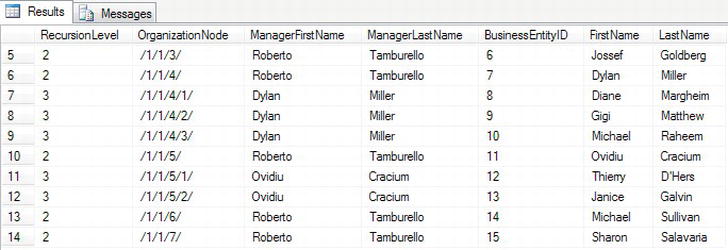
Figure 14-9. Recursive CTE output demonstrating hierarchical employees
Pivoting Data
If you have ever used Excel, then you have probably had to pivot data results so that rows of information are pivoted into columns of information. It is now possible to perform this kind of operation within SQL Server via a PIVOT operator. Pivoted data can also be changed back using the UNPIVOT operator, where columns of data can be changed into rows of data. In this section, you will see both of these in action. You will be using the AdventureWorks example in this section. The table involved in this example is the SalesOrderDetail table belonging to the Sales schema. This holds details of products ordered, the quantity requested, the price they are at, and the discount on the order received.T–SQL code
PIVOT
Before you see PIVOT in action, you need to look at the information that you will pivot. The following code lists three products, and for each product, you will sum up the amount sold, taking the discount into account:
SELECT ProductID,UnitPriceDiscount,SUM(LineTotal)

  FROM Sales.SalesOrderDetail

  WHERE ProductID IN (776,711,747)

  GROUP BY ProductID,UnitPriceDiscount

  ORDER BY ProductID,UnitPriceDiscount
This produces one line of output for each product/discount combination, as you can see in the following results:
711     0.00    143788.908000

711     0.02    11421.237324

711     0.05    4384.931245

711     0.10    2679.760530

711     0.15    3131.779950

747     0.00    501788.197700

776     0.00    1198796.448000

776     0.02    23020.131792

776     0.35    32906.152500
By using PIVOT, you can alter this data so that you can create columns for each of the products. Each row is defined for the discount, giving a cross-reference of products to discount.
SELECT pt.Discount,ISNULL([711],0.00) As Product711,

    ISNULL([747],0.00) As Product747,ISNULL([776],0.00) As Product776

FROM

(SELECT sod.LineTotal, sod.ProductID, sod.UnitPriceDiscount as Discount

   FROM Sales.SalesOrderDetail sod) so

PIVOT

(

SUM(so.LineTotal)

FOR so.ProductID IN ([776], [711], [747])

) AS pt

ORDER BY pt.Discount
Before you execute this code, let’s take a look at what is happening. First of all, you need to create a subquery that contains the columns of data that the PIVOT operator can use for its aggregation (it will also be used later for displaying in the output). No filtering has been completed at this point—any columns not used in the aggregation will be ignored. The code generates a table-valued expression with an alias of so. From this table, you then instruct SQL Server to PIVOT the columns while completing an aggregation on a specific column—in your case, a SUM of the LineTotal column from the table-valued expression. It is also at this point you define the columns to create via the FOR clause—in your case, a column for each product of the three products. This is the equivalent to using GROUP BY for the aggregation, and it’s also the equivalent of filtering data from the so table-valued expression. However, within the so table-valued expression, there’s also a third column, UnitPriceDiscount. Without this, the output from the PIVOT would produce one row with three columns—one for each product. So this table-valued expression with the PIVOT operation produces a temporary result set, which you name pt. You can then use this temporary result set to produce your output.
When you run the code, you should see output similar to what is shown in Figure 14-10.
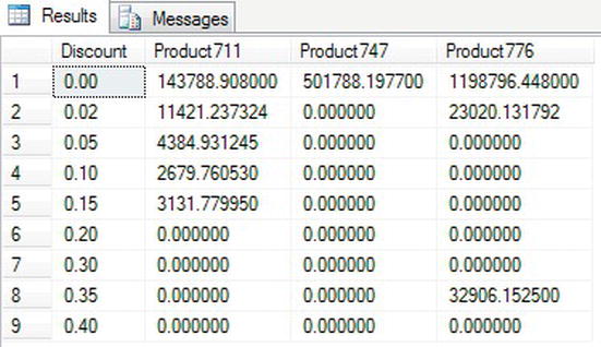
Figure 14-10. Pivot data results
UNPIVOT
The reverse of PIVOT is, of course, UNPIVOT, which will unpivot data by placing column data into rows. You can prove this by unpivoting the data just pivoted using the preceding query. The code that follows will rebuild the pivot and place the data into a temporary table. From that temporary table, you can unpivot the data.
![]() Note Although
Note Although PIVOT aggregates multiple rows into a single row in the output, UNPIVOT does not reproduce the original table-valued expression result because the rows have been aggregated. Besides, NULL values in the input of UNPIVOT disappear in the output, whereas there may have been original NULL values in the input before the PIVOT operation and the original structure has been lost.
SELECT pt.Discount,ISNULL([711],0.00) As Product711,

    ISNULL([747],0.00) As Product747,ISNULL([776],0.00) As Product776

INTO #Temp1

FROM

(SELECT sod.LineTotal, sod.ProductID, sod.UnitPriceDiscount as Discount

   FROM Sales.SalesOrderDetail sod) so

PIVOT

(

SUM(so.LineTotal)

FOR so.ProductID IN ([776], [711], [747])

) AS pt

ORDER BY pt.Discount
UNPIVOT has similarities to PIVOT in that you build a table-valued expression—in this case, calling it up1—which you then use as the basis of unpivoting. Once the table-valued expression is defined, you use UNPIVOT with the column definitions of the columns to create, DiscountAppl and ProductID. Using IN defines the rows that will be produced back from the UNPIVOT.
SELECT ProductID,Discount, DiscountAppl

  FROM (SELECT Discount, Product711, Product747, Product776

          FROM #Temp1) up1

UNPIVOT ( DiscountAppl FOR ProductID

    IN (Product711, Product747, Product776)) As upv2

WHERE DiscountAppl <> 0

ORDER BY ProductID
When the preceding code (both sections) is executed, the data are unpivoted, as shown in Figure 14-11.
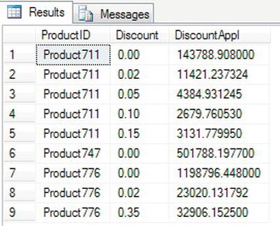
Figure 14-11. Unpivoted data results
Now that you have pivoted data, you can take a look at how you can rank output.
Ranking Functions
With SQL Server, it’s possible to rank rows of data in your T-SQL code. Ranking functions give you the ability to rank each row of data to provide a method of organizing the output in an ascending sequence. You can give each row a unique number or each group of similar rows the same number. You may be wondering what is wrong with other methods of ranking data, which might include IDENTITY columns. These types of columns do provide unique numbers, but gaps can form. You are also tied into each row having its own number, when you may want to group rows together.
So then, why not use GROUP BY? Well, yes, you can use GROUP BY, but what if the grouping was over more than one column? In this case, processing the data further would require knowledge about those columns. Ranking functions make it possible to provide a value that allows data to be ranked in the order required, and then that value can be used for splitting the data into further groupings.
There are four ranking functions, which I’ll discuss in detail in upcoming sections:
ROW_NUMBER: Allows you to provide sequential integer values to the result rows of a queryRANK: Provides an ascending, nonunique ranking number to a set of rows, giving the same number to a row of the same value as another; numbers are skipped for the number of rows that have the same value.DENSE_RANK: This is similar toRANK, but each row number returned will be one greater than the previous setting, no matter how many rows are the same.NTILE: This takes the rows from the query and places them into an equal (or as close to equal as possible) number of specified numbered groups, whereNTILEreturns the group number the row belongs to.
![]() Note These ranking functions can be used only with the
Note These ranking functions can be used only with the SELECT and ORDER BY statements. Sadly, they can’t be used directly in a WHERE or GROUP BY clause, but you can use them in a CTE or derived table.
The following code demonstrates a CTE with the ranking function ROW_NUMBER():
WITH OrderedOrders AS

(SELECT SalesOrderID, OrderDate,

ROW_NUMBER() OVER (order by OrderDate)as RowNumber

FROM Sales.SalesOrderHeader )

SELECT *

FROM OrderedOrders

WHERE RowNumber between 50 and 60
The syntax for ranking functions is shown as follows:
<function_name>() OVER([PARTITION BY <partition_by_list>]

ORDER BY <order_by_list>)
Taking each option as it comes, you can see how this can be placed within a SELECT statement—for example:
function_name: Can be one ofROW_NUMBER,RANK,DENSE_RANK, andNTILEOVER: Defines the details of how the ranking should order or split the dataPARTITION BY: Details which data the column should use as the basis of the splitsORDER BY: Details the ordering of the data
ROW_NUMBER
Your first ranking function, ROW_NUMBER, allows your code to guarantee an ascending sequence of numbers to give each row a unique number. Until now, it has not been possible to guarantee sequencing of numbers, although an IDENTITY-based column could potentially give a sequence, providing all INSERTs succeeded and no DELETEs took place.
This function is ideal for giving your output a reference point—for example, “Please take a look at row 10 and you’ll see. . .” Another use for this function is to break the data into exact chunks for scrolling purposes in GUI systems. For example, if five rows of data are returned, row 1 could be displayed, and then Next would allow the application to move to row 2 easily rather than using some other method.
The following is an example that shows how the ROW_NUMBER() function can provide an ascending number for each row returned when inspecting. The ROW_NUMBER() function is nondeterministic, and since the ORDER BY within the OVER function doesn’t produce a unique sequence of data (because there might be several people with the same last name, for example), then you would need to find some other way to achieve uniqueness, if getting the same order with each execution were mandatory.
![]() Note The following code and all code from this point is from the
Note The following code and all code from this point is from the ApressFinancial database.
USE ApressFinancial

GO

SELECT ROW_NUMBER() OVER (ORDER BY LastName) AS RowNum,

       CONCAT(FirstName,' ',LastName) AS CustomerName,

           UnclearedBalance

  FROM CustomerDetails.Customers

 WHERE UnclearedBalance is not null
When you execute the code, you see the names in last name order, as shown in Figure 14-12.
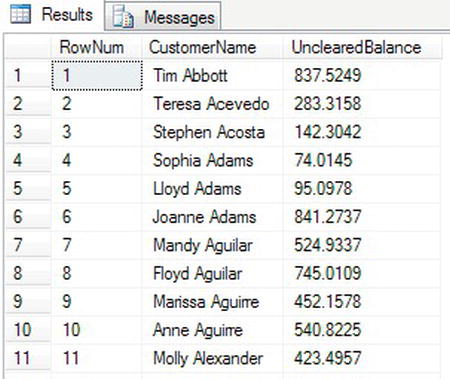
Figure 14-12. Rows with row numbering
It’s also possible to reset the sequence to give a unique ascending number within a section, or partition of data, using the PARTITION BY option. This would be ideal if, for example, in the same marathon you had different races, such as male, female, disabled male, disabled female, over 60, and so on. Using the category the runner is competing within as the basis of the partition, no matter in which order the runners cross the line, you would still have the correct order of finishing for each category.
The following example will reset the sequential number at each change of first letter in the last name of the employees and will order the results in LastName descending order:
SELECT ROW_NUMBER() OVER (PARTITION BY SUBSTRING(LastName,1,1)

       ORDER BY LastName) AS RowNum,

       CONCAT(FirstName,' ',LastName) AS CustomerName,

           UnclearedBalance

  FROM CustomerDetails.Customers

 WHERE UnclearedBalance is not null

 ORDER BY LastName DESC
When you execute the code, as the first letter of the last name alters, you see the RowNum column, which contains the value for ROW_NUMBER(), alter, as shown in Figure 14-13. However, you will also see a side effect that can happen when you include an ORDER BY statement within the code, which is the row numbering can become random. This occurs because the ordering of the results occurs after the data have been returned from the underlying table and the sequencing has been applied.
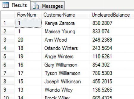
Figure 14-13. Rows with row numbering resetting on change of last name, first letter
It is possible to see how SQL Server processes your query by inspecting the query plan diagram. If you click the Include Actual Execution Plan button on your toolbar, this will display the query plan for the foregoing code once it is executed. After clicking the button, if you execute the previous code, there will be a new tab called Execution Plan. By selecting this tab, you will see something similar to Figure 14-14. A query plan works right to left; therefore the final result is the icon that is known as the step on the far left. There are two Sort steps within the plan. The Sort on the right is used to sort the data ready to be passed to the Segment and Sequence Project steps, and the Sort on the left is used to order the data.
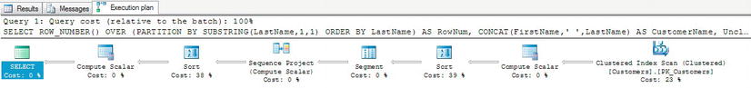
Figure 14-14. Query plan demonstrating ROW_NUMBER and ORDER BY DESC out of sequence
You can add the RowNum alias to specify the first column to the ORDER BY statement to be descending, as this will correct the sequencing if this is required.
RANK
If a row of data is returned that contains the same values as another row as defined in the ORDER BY clause of your statement, the keyword RANK will give these rows the same numerical value. An internal count is kept so that on a change of value, you will see a jump in the value. For example, say you watch a sport like golf, and in a golf tournament you’re following Tiger Woods, who wins the tournament on a score of 4 under par, but Lee Westwood, Luke Donald, and Phil Mickelson are tied for second at 3 under par. Finally, Bubba Watson finishes his round at 2 under par. Tiger would have the value 1; Lee, Luke, and Phil would have the value 2; and Bubba would have the value 5. This is exactly what RANK does. This function would also be useful in applications that wanted to return different rankings of data but show only the data from one rank at any one time on each page.
In the following example, the ROW_NUMBER() function is also used as it was in the previous example, enabling a cross-check where the RANK function skips to the right number. The SUBSTRING has also been altered from the previous example to look at the first two characters to enable a good demonstration of RANK. When you run the query, you’ll find that there is one row with a LastName that starts Ab. RANK will assign this row the number 1. When the LastName changes to Ac, the RANK will change to the value 2. After these two rows, you will see the RANK change to 4.
SELECT ROW_NUMBER() OVER (PARTITION BY SUBSTRING(LastName,1,2)

       ORDER BY LastName) AS RowNum,

           RANK() OVER(ORDER BY SUBSTRING(LastName,1,2) ) AS Ranking,

       CONCAT(FirstName,' ',LastName) AS CustomerName,

           UnclearedBalance

  FROM CustomerDetails.Customers

 WHERE UnclearedBalance is not null

 ORDER BY Ranking
Partial results are shown in Figure 14-15, where you can see in the Ranking column that the values remain static when the values are the same, and then skip to the correct number on a change of value.
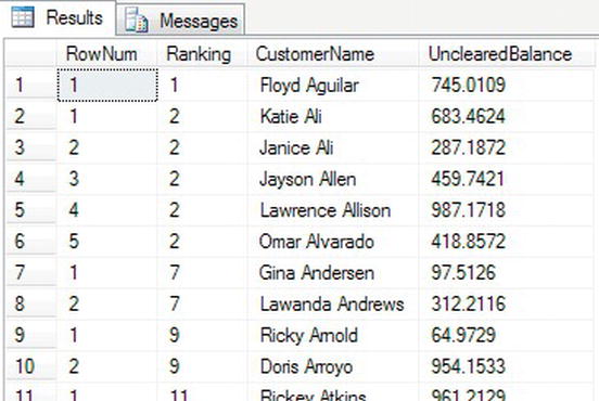
Figure 14-15. Ranking and row numbering
DENSE_RANK
DENSE_RANK gives each group the next number in the sequence and does not jump forward if there is more than one item in a group. In the golf example from the previous section, for example, Bubba Watson would have a value of 3 instead of a value of 5 because his score is the third highest. The following code demonstrates DENSE_RANK:
SELECT ROW_NUMBER() OVER (PARTITION BY SUBSTRING(LastName,1,2)

       ORDER BY LastName) AS RowNum,

           DENSE_RANK() OVER(ORDER BY SUBSTRING(LastName,1,2) ) AS Ranking,

       CONCAT(FirstName,' ',LastName) AS CustomerName,

           UnclearedBalance

  FROM CustomerDetails.Customers

 WHERE UnclearedBalance is not null

 ORDER BY Ranking
The results can be seen in Figure 14-16. Notice that this time, on change of the first two characters of the column LastName, the Ranking becomes 3 when Ac becomes Ad, instead of moving to 4.
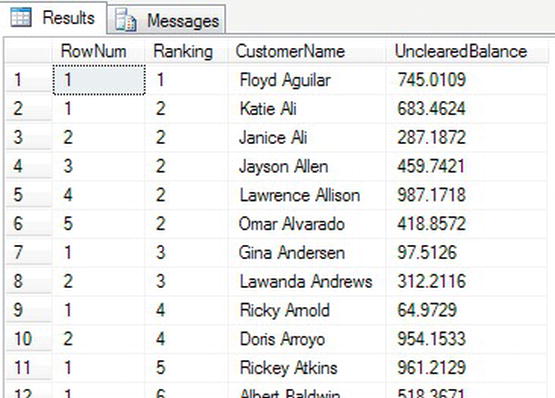
Figure 14-16. Dense ranking and row numbering
NTILE
Batching output into manageable groups has always been tricky. For example, if you have a batch of work that needs cross-checking among a number of people, then GROUP BY has to be used, though this wouldn’t give an even split. NTILE is used to give the split a more even, although approximated, grouping. The value in parentheses after NTILE defines the number of groups to produce, so NTILE(25) would produce 25 groups of as close a split as possible of even numbers.
SELECT NTILE(10) OVER (ORDER BY LastName) AS BatchNumber,

       CONCAT(FirstName,' ',LastName) AS CustomerName,

           UnclearedBalance

  FROM CustomerDetails.Customers

 WHERE UnclearedBalance is not null

 ORDER BY BatchNumber
This produces 10 groups of 99 rows each. In Figure 14-17, you will see where the first batch ends and the second batch commences.
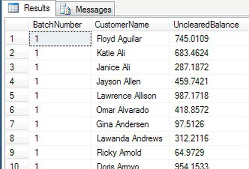
Figure 14-17. Batching output into groups of data
Cursors
SQL Server works best with sets of data. So far in the book, this is what you have seen demonstrated. However, there will be occasions when you need to work with a set of data a row at a time, and this is when you will need to work with cursors. A cursor builds a set of data based on a SELECT statement, which can then be read a row at a time.
Cursors are quite powerful and avoid passing a large set of data across a network, to then be processed with a development language such as .NET a row at a time, and then the resulting information passed back to SQL Server. Cursors can also update the underlying table data a row at a time if this is required. They can also be navigated to relative and specific positions within the set of data within the cursor. This can lead a SQL Server developer to think that they are the answer to all problems, but there are downsides. Cursors can and almost always are slower than using sets of data, and although they should not be avoided, they should not be approached lightly.
Let’s take a look at the syntax.
There are a number of options when declaring a cursor, and in this section you will see what each option will do. The cursor declaration is as follows:
DECLARE cursor_name CURSOR [ LOCAL | GLOBAL ]

     [ FORWARD_ONLY | SCROLL ]

     [ STATIC | KEYSET | DYNAMIC | FAST_FORWARD ]

     [ READ_ONLY | SCROLL_LOCKS | OPTIMISTIC ]

     [ TYPE_WARNING ]
     FOR select_statement

     [ FOR UPDATE [ OF column_name [ ,...n ] ] ]
The options are as follows:
cursor_name: The name of the cursor that will then be referenced with the other cursor statementsLOCAL|GLOBAL: Similar to temporary tables, there are two scopes for cursors, the local connection or the global connection. Local is the default.FORWARD ONLY|SCROLL: Forward indicates only that you are scrolling a row at a time from the start of the cursor to the end. This is the default. TheSCROLLoption indicates that you can move forward, backward, first, last, and to a specific position.STATIC|KEYSET|DYNAMIC|FAST FORWARD: If any of these options are defined, then the default on the foregoing option isSCROLL.-
STATIC: A temporary copy of the data is placed intotempdb. Therefore within your cursor or in an external process any updates to the base tables will be outside of the cursor. This is ideal if you are running a cursor when modifications to the underlying tables could occur and you don’t want to process the updates.STATICis the default. -
KEYSET: All tables defined within a cursor that has theKEYSEToption must have a unique key. The unique key values are copied totempdb. Data altered in nonkey value columns are visible provided the changes are within the cursor. Changes made outside the cursor are not visible. Changes to key values can result in a -2@@FETCH_STATUS, row not found. -
DYNAMIC: While you are scrolling through a cursor fetching rows, the data within the cursor are not static and any updates to the underlying tables would be reflected within the cursor. You have to be aware that more rows could be added while you are scrolling through, and you may also retrieve a row that you retrieved earlier if the values have been altered so that they would be refound. For example, if you ordered the cursor to be in an order of last updated and you updated the column withGETDATE(), you would retrieve the row again as it would be placed at the end of the cursor. -
FAST FORWARD: A performance-enhanced, forward-only, read-only cursor
-
READ ONLY|SCROLL LOCKS|OPTIMISTIC-
READ ONLY: The cursor is read-only and cannot be updated. -
SCROLL LOCKS: For update cursors, a lock is placed on the rows within the cursor to ensure that updates succeed. This will block any other process that wants access to the underlying data until the cursor lock is released with theDEALLOCATEcommand. This can mean just the row being locked, but it can also mean that the whole table or multiple tables are locked. -
OPTIMISTIC: If you believe that any rows that you update within the cursor will succeed, you can select optimistic locking. What this means is that when the cursor is opened, rows are not locked at this point, but when updated, the row is checked against the base table. If the row has not been updated since the cursor was opened, then the update will succeed. If the row has been updated, then the update will fail.
-
TYPE WARNING: A warning message will be sent when a cursor is implicitly converted from one type to another. Sometimes SQL Server will convert a cursor to another type of cursor. This isn’t an error but a warning. An example would be where you define a cursor asKEYSETbut one of the tables does not have a unique index, the cursor would change toSTATIC.FOR select_statement: TheSELECTstatement used to return the rows to build the cursorFOR UPDATE: If you want your cursor to be able to update the underlying tables, then you would define the cursor with this option.OF column_name: If you want only some columns updated, then you would list them with theOFoption. Without this option defined, all columns within the cursor can be modified.
Once the cursor is declared, there are a number of steps that should be followed to work with your cursor effectively. The steps in order are as follows:
OPEN cursor_name: Once a cursor is declared, you do need to open it. If you don’t open it, an error will occur when you try to read from it. TheOPENpopulates the cursor, not theDECLARE.FETCH NEXT FROM cursor_name [INTO @variables]: Once the cursor is opened, you then need to fetch each row from the cursor. If you want to work with the data, you would retrieve from the cursor into local variables. To display the data only rather than work with the values in variables, you can omit the variables and each row will be output. This is useful if you are wishing to append information like aSELECTcan output column values for each row rather than working with the values. Note that you must fetch for the first time before processing a row. The first row will not be automatically read.@@FETCH_STATUS: The SQL Server status of the cursor. This is used as the test while looping around each cursor row until you reach the end. A value of 0 means that the row was returned successfully; a value of -1 indicates you are at the end of the cursor; and a value of -2 means that the cursor row was missing. You would see this value in an updatable cursor and if the row expected was no longer there in the cursor.CLOSE cursor_name: Once you have finished with the cursor, close it to release locks. The cursor remains and could be reopened and the data refetched if you wished.DEALLOCATE cursor_name: Releases the data structures and therefore the cursor allocation and the used resources back to SQL Server
Now that you have the syntax for a cursor and the constituent parts of building code for a cursor, the next exercise will see these parts brought together to create a forward-only cursor. The code will be broken out in steps and then once complete will be executed. Finally, at the end, do keep the code handy as it will be used in the next section on debugging.
TRY IT OUT: BUILDING AND RUNNING A CURSOR
The first cursor option that you will see is a read-only, forward-only cursor. This will be modified in the subsequent examples for other options.
- The first section of code will define the variables to hold the data from each of the columns of the cursor. There is also a local variable required to keep a running total of the amount collected. The variable used for this is
@TotalCollectedand is initialized to0.DECLARE @FirstName varchar(50), @LastName varchar(50),
@ProductName nvarchar(50), @Amount money,
@LastCollect datetime
DECLARE @TotalCollected money = 0 - The next step is to declare the cursor name and the
SELECTstatement to return the rows of data for the cursor. The aim of the cursor is to return rows where there is a monthly amount to collect from a customer, and the last amount collected was in March. Hard-coded dates are being used for simplicity, as aGETDATE()will differ depending on when you are reading this exercise.DECLARE FinProductsColl CURSOR
FOR SELECT c.FirstName, c.LastName, f.ProductName,
cp.AmountToCollect, cp.LastCollected
FROM CustomerDetails.Customers c
JOIN CustomerDetails.CustomerProducts cp
ON cp.CustomerId = c.CustomerId
JOIN CustomerDetails.FinancialProducts f
ON f.ProductId = cp.FinancialProductId
WHERE cp.Frequency = 2
AND cp.LastCollected BETWEEN '1 Mar 2012' AND '31 Mar 2012' - Once the cursor is declared, it can be opened, ready for processing.
OPEN FinProductsColl - The first action against the cursor is to retrieve the first row and place the data from the columns into local variables.
FETCH NEXT FROM FinProductsColl
INTO @FirstName, @LastName, @ProductName, @Amount, @LastCollect - You should then check the status of the
FETCHto ensure that a row has been returned. While a row is returned, loop around, and the loop is defined with theWHILEandBEGINstatements. - Now that you are confident you have a row, you can work with the data in the local variables from the row of data from the cursor. In this instance, the cursor is totaling the amount collected.
SELECT @TotalCollected = @TotalCollected + @Amount - The local variable values are listed for display. A conversion from the
moneydata type is required so that it can be concatenated with the other information.SELECT @FirstName, @LastName, @ProductName, @Amount,
'Running total is ' + CONVERT(varchar(20),@TotalCollected) - At the end of the loop, the next row from the cursor set is retrieved and the values placed into the local variables. The loop is closed with the
ENDstatement.FETCH NEXT FROM FinProductsColl
INTO @FirstName, @LastName, @ProductName, @Amount, @LastCollect
END - Once the loop completes, when
@@FETCH_STATUSis not zero, then you have finished processing the cursor, you can list out how much has been collected. The cursor is then closed and deallocated. This is the end of the code.SELECT 'Total collected is ' + CONVERT(varchar(20),@TotalCollected)
CLOSE FinProductsColl
DEALLOCATE FinProductsColl - You can now execute the code, and the results that can be found at the end showing the total collected are shown in Figure 14-18.
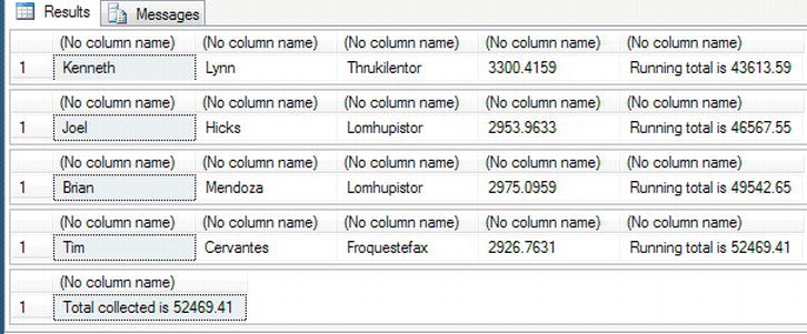
Figure 14-18. The end results showing the grand total
You can extend cursors to updatable cursors and other functionality, but you will mainly work with forward-only, read-only cursors. Just to clarify, some developers are quite scathing of cursors. Where possible, you should work with sets of data as this is how SQL Server performs best, but there will be times when you will have to work on a row at a time. As long as you are clear that set-based processing is not possible, then you should consider using a cursor. However, it is worth looking at updatable cursors, which you will see next.
Working with an Updatable Cursor
This exercise will take the customer products that require money to be collected, total the amount, and then update the underlying CustomerDetails.CustomerProducts table to indicate that the money has been collected by updating the LastCollected column. The code is surrounded by a transaction around the cursor and the updates, and the transaction is rolled back so that the underlying data remain static, so that you can run this test multiple times in case of a coding error. You can run it with a COMMIT if you want to complete a full check; however, the code will prove that an update to the underlying data has taken place and completed. The code is very close to that built in the read-only cursor, and I will break where there is a change for you to note.
- Start your code with the
BEGIN TRANand then the variable declarations. There is a new variable that will hold the date and time the collection was made, which is called@DateCollectionand will hold a static value.BEGIN TRAN
DECLARE @FirstName varchar(50), @LastName varchar(50),

        @ProductName nvarchar(50), @Amount money,

        @LastCollect datetime


DECLARE @TotalCollected money = 0, @DateCollected datetime = GETDATE() - This
SELECTstatement will use the same joins and filters as the cursor to ensure that the same data are returned as the cursor. It will show the date and time defined for the@DateCollectedvariable and a count of the number of rows. You could also use the@@CURSOR_ROWSvariable after the cursor is open; however, thisSELECTis defined to demonstrate that there are no smoke-and-mirrors in the example.SELECT @DateCollected, COUNT(*)
FROM CustomerDetails.Customers c
JOIN CustomerDetails.CustomerProducts cp
ON cp.CustomerId = c.CustomerId
JOIN CustomerDetails.FinancialProducts f
ON f.ProductId = cp.FinancialProductId
WHERE cp.Frequency = 2
AND cp.LastCollected BETWEEN '1 Mar 2012' AND '31 Mar 2012' - The cursor has two new options at the end.
FOR UPDATEshows that the underlying data can be modified, but the cursor allows only one column,LastCollected, to be modified. The code then moves on to open and work with the cursor. To reduce output, theSELECTstatement that outputs the variables from the cursor is commented out. I have put this in bold for ease.DECLARE FinProductsColl CURSOR
FOR SELECT c.FirstName, c.LastName, f.ProductName,
cp.AmountToCollect, cp.LastCollected
FROM CustomerDetails.Customers c
JOIN CustomerDetails.CustomerProducts cp
ON cp.CustomerId = c.CustomerId
JOIN CustomerDetails.FinancialProducts f
ON f.ProductId = cp.FinancialProductId
WHERE cp.Frequency = 2
AND cp.LastCollected BETWEEN '1 Mar 2012' AND '31 Mar 2012'
FOR UPDATE
OF LastCollected
OPEN FinProductsColl
FETCH NEXT FROM FinProductsColl

INTO @FirstName, @LastName, @ProductName, @Amount, @LastCollect
WHILE @@FETCH_STATUS = 0

BEGIN
SELECT @TotalCollected = @TotalCollected + @Amount
-- SELECT @FirstName, @LastName, @ProductName, @Amount,
-- 'Running total is ' + CONVERT(varchar(20),@TotalCollected) - Moving to the next new section of code, you will find the update to one of the underlying tables. To update within a cursor, you still define the table to modify but instead of finding the row with a
WHERE column = value, the faster method—and one that will update the same row as you are at within the cursor—is to useCURRENT OFand then the name of the cursor. The code then continues as the read-only cursor.UPDATE CustomerDetails.CustomerProducts
SET LastCollected = @DateCollected
WHERE CURRENT OF FinProductsColl
    FETCH NEXT FROM FinProductsColl

    INTO @FirstName, @LastName, @ProductName, @Amount, @LastCollect

END - Before completing the code, do a quick test to see if the same number of rows now has the
@DateCollecteddate and time as there was at the start of the example. - The transaction is rolled back.
ROLLBACK TRAN
SELECT 'Total collected is ' + CONVERT(varchar(20),@TotalCollected)

CLOSE FinProductsColl

DEALLOCATE FinProductsColl - When you execute the foregoing code, you should see something similar to Figure 14-19, where the number of rows should match in the first two result sets.
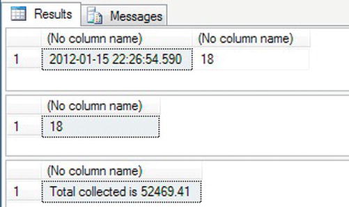
Figure 14-19. The test results from the updatable cursor
Let’s be clear: cursors are usually not the best way to work with your data, but there are times that you have to work a row at a time, and although slower than working with sets, it may be the best option for what is required. Never disregard cursors outright as some developers do.
Debugging Your Code
Now that you are at the point where you have the knowledge to build advanced T-SQL, you will be entering a stage of development where you will need to debug your code. So why and when do you need to debug code?
Debugging code can occur during development, testing, and even post-release. When you are developing your code, you may build a stored procedure a section at a time, checking that you have the information you expect at a specific point in time. It may be that you want to check that variables have the correct information before, during, or after execution. Or you may want to check that your CASE statements, loops, WHERE statements, etc. are all performing as expected. This can always be achieved by displaying information via a SELECT or PRINT statement, but these statements can be left behind in the stored procedure and inadvertently released to production. If you have the ability to step through your code a line or a block at a time, and when the code is paused to have the ability to inspect values in a transient way among many other features, this would eliminate code being released in error.
SQL Server 2012 has greatly improved the ability to debug your code and is very close to how code is debugged in Visual Studio. There are a number of options and windows that help you debug your code, which I will go through before displaying an example of how to debug your code.
There are a number of requirements to make a good debugger. You need to see your code and at what point of execution you are; be able to pause, or breakpoint, your code; be able to display and alter values of variables; and be able to step your code so you can execute a line of code at a time. All of these tasks should be simple to perform.
You can debug database code within Visual Studio, but the ability to debug code within SQL Server using Management Studio can help you to debug code in an easier fashion, because all of the work is being completed on SQL Server. A number of options are available from several areas of SSMS, giving you, as a developer, a good level of flexibility. The first area that is available is from the menu in SSMS when a code window is open. You can see the options in Figure 14-20.
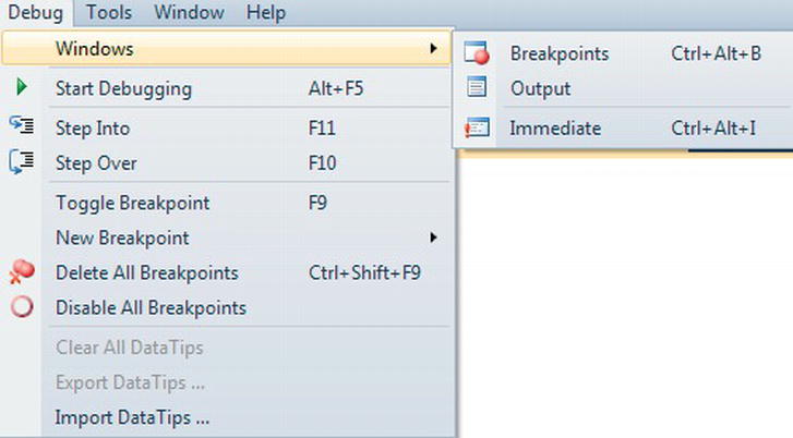
Figure 14-20. The Debug menu within SSMS
There are only three windows defined in the menu, but as you debug, then more windows become available, which I will cover in the next section.
Debugging Windows
Debug windows are ideal for viewing information or performing actions against code being debugged. Each window provides useful but specific information. The windows that are available are as follows:
- Call Stack: If you have nested stored procedures or you call functions, then the Call Stack window will show each object in a hierarchy. This will allow you to see via which route you reach the point in code that you have breakpointed at.
- Breakpoints: A breakpoint is an indicator in your code where you want SQL Server to pause execution. You can have one or more breakpoints within your code, and these are ideal for pausing your execution to inspect variables, check information, and generally decide how you want to proceed. Figure 14-21 shows the details of two breakpoints that you will set in the forthcoming example. The columns
Labels,Condition, andHit Countare covered in a few moments.
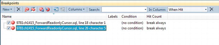
Figure 14-21. The Breakpoints window
- Command: Allows for commands to be executed; these are explicit commands, such as
Debug.AddWatchandDebug.StepInto. - Output: When setting a breakpoint, it is also possible to write out information at that time. You will see this in the forthcoming example, and output from the breakpoint will be placed in the output window.
- Immediate: Like the Command window, you can execute commands immediately, and you can also run stored procedures and other code immediately.
- Autos: This will show the variables like the local window but only variables in the current statement and the previous statement.
- Locals: This will automatically display any locally defined variables and their current values.
- Watch: If you have variables that you want to watch the values of as you process your code, then you would add these to the Watch window so that they are available. You can also alter the value of a variable within a Watch window if required to aid testing. You will see this in the example.
Now that the windows have been covered, you can take a look at the options available to you to debug your code.
Debugging Options
The ability to be in control of code execution is a cornerstone of debugging code. In this section, you will see the options available when debugging. A few of these options are available before you commence, as shown in Figure 14-20, but others will become enabled once debugging starts. The options are as follows:
- Show Next Statement: Highlight the next statement to execute; this is ideal when looping.
- Step Into: If you have a statement that calls another stored procedure or function, this option will step into the stored procedure where you can step through each line.
- Step Over: As an opposite to the Step Into option, the Step Over option will not step into the stored procedure and will execute the stored procedure or function, but you will not step through the code.
- Step Out: If you are in a lower-level stored procedure or function, by selecting this option, the remaining code for the stored procedure or function will run and you will then break at the line of code that called the stored procedure, ready to proceed to the next line.
- Toggle Breakpoint: Switch between a breakpoint being set, or removed on the line of code you are paused at; you can set a breakpoint by clicking in the left-hand margin of the code window.
- New Breakpoint: Define a function to breakpoint at; if you call the same function several times, a breakpoint will occur at this point at each call.
- Delete All Breakpoints: Remove all the breakpoints in your code
- Clear All DataTips: A datatip is where you highlight a variable within code and pin it within the code. This will then add a watch to the variable, but instead of being in a Watch window, it will be inline within the code. Clear All DataTips will remove from your code any tips that you have. A datatip is shown in Figure 14-22.
- Export DataTips: Once at least one datatip has been set, it can be exported so that any other developers can take those tips and import them for their own debugging. Also you can export the tips and store them in a source control system for debugging in the future.
- Import DataTips: Any exported datatips can be imported and used for debugging.
Figure 14-22. A datatip in code showing a value
So you are now well on the way to starting to debug your code.
Debugging Pop-Up Window
Once debugging starts, within the Query Editor window, a pop-up dialog becomes available. If you right-click, a pop-up, as shown in Figure 14-23, will be displayed. This gives you a number of further options for debugging based on the line of code the cursor is on. So although you may be breakpointed at one line of code, you can move the cursor to a different line of code and right-click, and you will be acting on that line of code instead of the breakpoint.
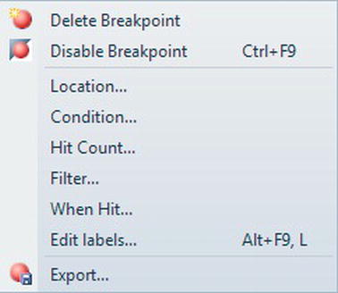
Figure 14-23. Debug options within Query Editor
The options are as follows:
- Delete Breakpoint: Remove the breakpoint so that the code will continue when that line of code is reached
- Disable Breakpoint: Keep the breakpoint for future debugging but disable the breakpoint
- Location…: Define a breakpoint by file, line, and character
- Condition…: Break when a condition is met or has altered; this is useful for when you want to track a variable, but you are not sure where it is changed.
- Hit Count…: Break your code when the line highlighted is “hit” the number of times defined when you click Hit Count; this can be useful for testing how a loop behaves in the middle of its iterations.
- Filter…: It is possible to breakpoint on a different process and thread. This is good for when you are calling code outside of your process.
- When Hit…: When the breakpoint is hit, output some information to the output window; you will see this demonstrated in the following example.
- Edit Labels…: It is possible to label your breakpoint. By default, breakpoints have no label, but by having the ability to label, you can have multiple breakpoints grouped and therefore make tracking of the breaks easier to follow. This is a bit like labeling nested transactions.
- Export…: Breakpoints can be exported and stored with your stored procedures or code so that they can exist for future debugging or as some sort of test evidence. Breakpoints are exported as an XML file.
Now that the options available for debugging your code have been covered, it is time to see debugging in action and put some of this information into an example. This exercise will show only a small amount of what is possible with debugging, as it would require a whole chapter to show everything in detail. You will see the fundamentals and enough for many situations.
TRY IT OUT: DEBUGGING CODE
If you have closed the forward-only, read-only cursor, then open it.
- Scroll to the
OPENcursor command and ensure the cursor is on that line of code. Click in the left-hand margin, and you should see a red dot, as shown in Figure 14-24. You should do the same at the line of code that updates the@TotalCollectedvariable.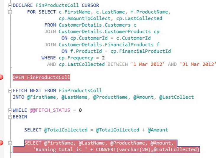
Figure 14-24. The two breakpoints within the code
- Click Debug from the toolbar at the top of Management Studio. It is to the right of the Execute button, as shown in Figure 14-25. You can also press Alt+F5.

Figure 14-25. The Debug toolbar option before debugging starts
- The Query Editor window should now change and look like Figure 14-26. A yellow line will be on the first line of code that is to be executed, and a yellow cursor appears in the left-hand margin. You will also see the windows described earlier appear at the foot of the screen.
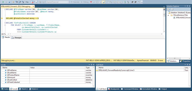
Figure 14-26. Debugging commenced with current line highlighted
- The first
DECLAREis not highlighted, as that is just defining variables and has no code that can be debugged. However, with the@TotalCollectedvariable, it is assigned a value and so SQL Server will breakpoint here. - If you move to the Locals screen, as shown in Figure 14-27, you will see the variables defined and each current value. Special attention is on
@TotalCollected, as you will see in the next step.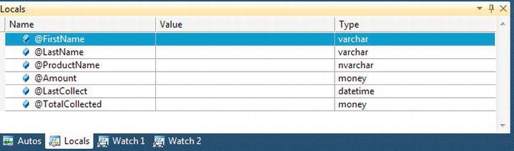
Figure 14-27. The Locals window showing the variables and their values
- Within the Locals window, you can alter the value a variable has; the
Valuecolumn is a toggle column between read and edit. By clicking the value twice, it will first highlight the value, and then toggle to edit. Once you have achieved this, alter the value to be 100, as shown in Figure 14-28.This will be overwritten to a value of 0 when the line you are paused at is run, as it will set the value to 0.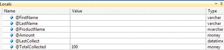
Figure 14-28. The Locals window with a value defined
- Now that you have the debugger started, and for your testing a value has been defined for a local variable, it is time to run to the first breakpoint, as shown in Figure 14-29. There are two ways to get to this point, either by stepping a line at a time via F10, or by pressing Alt+F5 or the green arrow on the toolbar. Both of these two options will continue running your code.
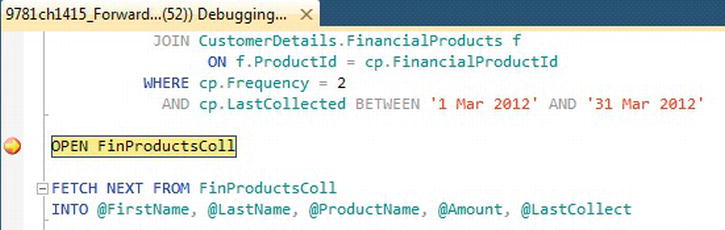
Figure 14-29. Hitting the first breakpoint
- Perform the same action to reach the second breakpoint, as shown in Figure 14-30.
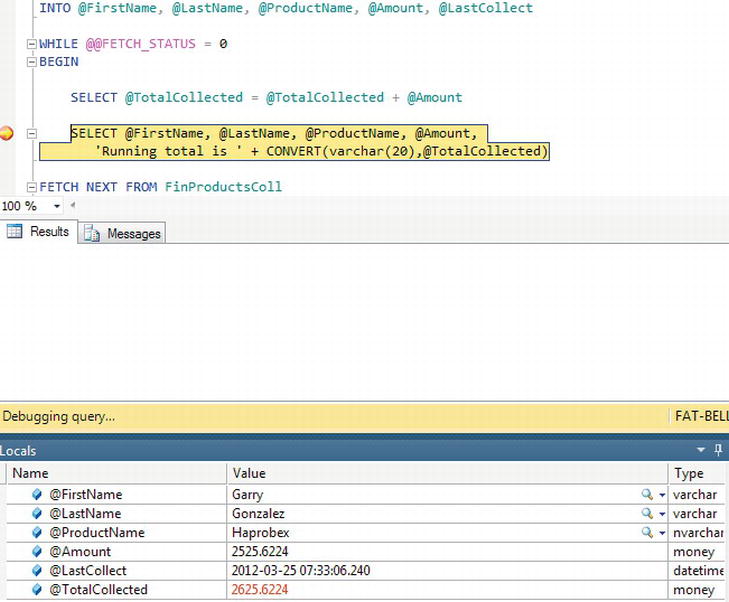
Figure 14-30. The second breakpoint where a row from the cursor is being processed
- Notice that the Locals window now has values for the local variables taken from the cursor row and that the
@TotalCollectedvariable has increased by the@Amountvariable. - Before moving on, rather than breakpointing each time you loop around the cursor to check the value in the variable, you can output information to the Output window when this line of code is hit. Move to the left-hand margin and right-click. This will display the pop-up window as shown in Figure 14-31 and discussed earlier.
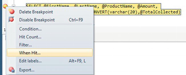
Figure 14-31. Debug pop-up window
Note The link of When Hit… does not need to be a breakpoint line. - From the window that is displayed, you can enter relevant text. Within the window, you will see some predefined variable options that you can put in the text, as shown in Figure 14-32. Enter the following text into the “Print a message” text box. The “Continue execution” check box will automatically select.
Function: $FUNCTION, Breakpoint hit - TotalCollected is {@TotalCollected}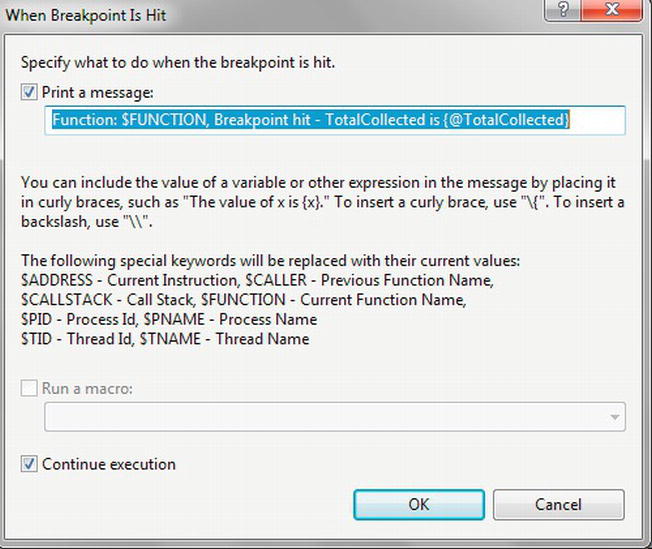
Figure 14-32. When Breakpoint Is Hit window with the required text to output
- This will remove the breakpoint so that the code will not break each time it is hit.
- Press Alt+F5 or click the green arrow. This will instruct the debugger to continue processing, and as there are no more breakpoints, execution will complete.
- If you look at the output window, you will see the information from the When Hit… Only part of the output is displayed here.
Function: 9781ch1415_ForwardReadonlyCursor.sql, Breakpoint hit –

TotalCollected is 2625.6224

Function: 9781ch1415_ForwardReadonlyCursor.sql, Breakpoint hit - TotalCollected is 5298.1525

Function: 9781ch1415_ForwardReadonlyCursor.sql, Breakpoint hit –

TotalCollected is 8372.6048

Function: 9781ch1415_ForwardReadonlyCursor.sql, Breakpoint hit –

TotalCollected is 10658.8615
This concludes the introduction and details about debugging and completes the chapter. Debugging is detective work, so exactly what debugging statements you need will depend on the specific circumstances. It is a crucial tool for a developer, and you can expect to use a debugger as much as any other area of SQL Server that you have seen.
Summary
The comparison of sequences with IDENTITY was explored and demonstrated, showing how sequences can be a better and more flexible alternative. They are not a replacement for IDENTITY columns, and you should now have the knowledge of when to use sequences instead of IDENTITY.
Subqueries are one of the most commonly used areas of T-SQL, but common table expressions are also useful, so knowing these areas well will enable you to move forward at a rapid pace. Combine this knowledge with the functionality covered in Chapter 11, especially when working with JOINs, and you should be able to see how powerful T-SQL can be at working with time-based data.
Throughout the book, you have looked at set-at-a-time processing, but in this chapter, you saw how to work with data a row at a time via cursors. Cursors are not something that should be avoided, but you need to take care and know when to use a cursor, which is slower than set-at–a-time, and when not to.
One of the final areas you looked at was how to debug your code. Setting breakpoints and the ability to view values within variables are “must-have” knowledge to give you the power to test your code. The ability to export breakpoints and datatips will allow future testing to take place but will also allow others to help debug your code if help is required.
One last piece of advice: If a query starts becoming very complex, you may find that it starts performing badly. We won’t look at performance of queries within this book, although I have discussed indexes and how they can help your query perform better. Always take a step back and think, “Would this work better as two queries, where the first query creates a subset of data?” Writing the most complex of queries that process all the data in one pass of the data may not always be the best answer.
You are coming to the end of the book, and you are well primed with T-SQL knowledge of what you can achieve with stored procedures and functions. In Chapter 15, you will take a look at triggers, and all you have learned with programming T-SQL can be applied there as well.