
![]()
Designing and Tuning the Indexes
It is impossible to define an indexing strategy that will work everywhere. Every system is unique and requires its own indexing approach. However, there are several design considerations and guidelines that can be applied in every system.
The same is true when we are optimizing existing systems. While optimization is an iterative process, which is unique in every case, there is the set of techniques that can be used to detect inefficiencies in every database system.
In this chapter, we will cover a few important factors that you will need to keep in mind when designing new indexes and optimizing existing systems.
Clustered Index Design Considerations
There are several design guidelines that help when choosing an efficient clustered index. Let’s discuss them now in detail.
Design Guidelines
Every time you change the value of a clustered index key, two things happen. First, SQL Server moves the row to a different place in the clustered index page chain and the data file. Second, it updates the row-id, which is the clustered index key, and is stored and needs to be updated in all nonclustered indexes. That can be expensive in terms of I/O, especially in the case of batch updates. Moreover, it can increase the fragmentation of the clustered index and, in case of row-id size increase, a nonclustered indexes. Thus it is better to have a static clustered index when key values do not change.
All nonclustered indexes use a clustered index key as the row-id. A too wide clustered index key increases the size of nonclustered index rows and requires more space to store them. As a result, SQL Server needs to process more data pages during index or range scan operations, which makes the index less efficient.
Performance of singleton lookups are usually not affected by a wide row-id with one possible exception: when a nonclustered index has not been defined as unique, it will store the row-id on non-leaf levels, which can lead to extra intermediate levels in the index. Even though non-leaf index levels are usually cached in memory, it introduces additional logical reads every time SQL Server traverses the nonclustered index B-Tree.
Finally, larger nonclustered indexes use more space in the buffer pool and introduce more overhead during index maintenance. Obviously, it is impossible to provide a generic threshold value that defines the maximum acceptable size of the key and that can be applied to any table. However, as the general rule, it is better to have a narrow clustered index key with the index key as small as possible.
It is also beneficial to have the clustered index defined as unique. The reason this is important is not obvious. Consider the scenario when a table does not have a unique clustered index and you want to run a query that uses nonclustered index seek in the execution plan. In this case, if the row-id in the nonclustered index were not unique, SQL Server would not know what clustered index row to choose during the key lookup operation.
SQL Server solves such problems by adding another nullable integer column called uniquifier to non-unique clustered indexes. SQL Server populates uniquifiers with NULL for the first occurrence of the key value, autoincrementing it for each subsequent duplicate inserted into the table.
![]() Note The number of possible duplicates per clustered index key value is limited by integer domain values. You cannot have more than 2,147,483,648 rows with the same clustered index key. This is a theoretical limit, and it is clearly a bad idea to create indexes with such poor selectivity.
Note The number of possible duplicates per clustered index key value is limited by integer domain values. You cannot have more than 2,147,483,648 rows with the same clustered index key. This is a theoretical limit, and it is clearly a bad idea to create indexes with such poor selectivity.
Let’s look at the overhead introduced by uniquifiers in non-unique clustered indexes. The code shown in Listing 6-1 creates three different tables of the same structure and populates them with 65,536 rows each. Table dbo.UniqueCI is the only table with a unique clustered index defined. Table dbo.NonUniqueCINoDups does not have any duplicated key values. Finally, table dbo.NonUniqueCDups has a large number of duplicates in the index.
Listing 6-1. Nonunique clustered index: Table creation
create table dbo.UniqueCI
(
        KeyValue int not null,
        ID int not null,
        Data char(986) null,
        VarData varchar(32) not null
                constraint DEF_UniqueCI_VarData
                default 'Data'
);

create unique clustered index IDX_UniqueCI_KeyValue
on dbo.UniqueCI(KeyValue);

create table dbo.NonUniqueCINoDups
(
        KeyValue int not null,
        ID int not null,
        Data char(986) null,
        VarData varchar(32) not null
                constraint DEF_NonUniqueCINoDups_VarData
                default 'Data'
);

create /*unique*/ clustered index IDX_NonUniqueCINoDups_KeyValue
on dbo.NonUniqueCINoDups(KeyValue);

create table dbo.NonUniqueCIDups
(
        KeyValue int not null,
        ID int not null,
        Data char(986) null,
        VarData varchar(32) not null
                constraint DEF_NonUniqueCIDups_VarData
                default 'Data'
);

create /*unique*/ clustered index IDX_NonUniqueCIDups_KeyValue
on dbo.NonUniqueCIDups(KeyValue);

-- Populating data
;with N1(C) as (select 0 union all select 0) -- 2 rows
,N2(C) as (select 0 from N1 as T1 CROSS JOIN N1 as T2) -- 4 rows
,N3(C) as (select 0 from N2 as T1 CROSS JOIN N2 as T2) -- 16 rows
,N4(C) as (select 0 from N3 as T1 CROSS JOIN N3 as T2) -- 256 rows
,N5(C) as (select 0 from N4 as T1 CROSS JOIN N4 as T2) -- 65,536 rows
,IDs(ID) as (select row_number() over (order by (select NULL)) from N5)
insert into dbo.UniqueCI(KeyValue, ID)
        select ID, ID
        from IDs;

insert into dbo.NonUniqueCINoDups(KeyValue, ID)
        select KeyValue, ID
        from dbo.UniqueCI;

insert into dbo.NonUniqueCIDups(KeyValue, ID)
        select KeyValue % 10, ID
        from dbo.UniqueCI;
Now let’s look at the clustered indexes physical statistics for each table. The code for this is shown in Listing 6-2, and the results are shown in Figure 6-1.
Listing 6-2. Nonunique clustered index: Checking clustered indexes row size
select index_level, page_count, min_record_size_in_bytes as [min row size]
        ,max_record_size_in_bytes as [max row size]
        ,avg_record_size_in_bytes as [avg row size]
from sys.dm_db_index_physical_stats
(db_id(), object_id(N'dbo.UniqueCI'), 1, null , 'DETAILED')

select index_level, page_count, min_record_size_in_bytes as [min row size]
        ,max_record_size_in_bytes as [max row size]
        ,avg_record_size_in_bytes as [avg row size]
from sys.dm_db_index_physical_stats
(db_id(), object_id(N'dbo.NonUniqueCINoDups'), 1, null , 'DETAILED')

select index_level, page_count, min_record_size_in_bytes as [min row size]
        ,max_record_size_in_bytes as [max row size]
        ,avg_record_size_in_bytes as [avg row size]
from sys.dm_db_index_physical_stats
(db_id(), object_id(N'dbo.NonUniqueCIDups'), 1, null , 'DETAILED')

Figure 6-1. Nonunique clustered index: Clustered indexes row size
Even though there is no duplicated key values in the dbo.NonUniqueCINoDups table, there are still two extra bytes added to the row. SQL Server stores a uniquifier in variable-length sections of the data, and those two bytes are added by another entry in a variable-length data offset array.
In this case, when a clustered index has duplicate values, uniquifiers add another four bytes, which makes for an overhead of six bytes total.
It is worth mentioning that in some edge cases, the extra storage space used by the uniquifier can reduce the number of the rows that can fit into the data page. Our example demonstrates such a condition. As you can see, dbo.UniqueCI uses about 15 percent fewer data pages than the other two tables.
Now let’s see how the uniquifier affects nonclustered indexes. The code shown in Listing 6-3 creates nonclustered indexes in all three tables. Figure 6-2 shows physical statistics for those indexes.
Listing 6-3. Nonunique clustered index: Checking nonclustered indexes row size
create nonclustered index IDX_UniqueCI_ID
on dbo.UniqueCI(ID);

create nonclustered index IDX_NonUniqueCINoDups_ID
on dbo.NonUniqueCINoDups(ID);

create nonclustered index IDX_NonUniqueCIDups_ID
on dbo.NonUniqueCIDups(ID);

select index_level, page_count, min_record_size_in_bytes as [min row size]
        ,max_record_size_in_bytes as [max row size]
        ,avg_record_size_in_bytes as [avg row size]
from sys.dm_db_index_physical_stats
(db_id(), object_id(N'dbo.UniqueCI'), 2, null , 'DETAILED')

select index_level, page_count, min_record_size_in_bytes as [min row size]
        ,max_record_size_in_bytes as [max row size]
        ,avg_record_size_in_bytes as [avg row size]
from sys.dm_db_index_physical_stats
(db_id(), object_id(N'dbo.NonUniqueCINoDups'), 2, null , 'DETAILED')

select index_level, page_count, min_record_size_in_bytes as [min row size]
        ,max_record_size_in_bytes as [max row size]
        ,avg_record_size_in_bytes as [avg row size]
from sys.dm_db_index_physical_stats
(db_id(), object_id(N'dbo.NonUniqueCIDups'), 2, null , 'DETAILED')
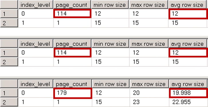
Figure 6-2. Nonunique clustered index: Nonclustered indexes row size
There is no overhead in the nonclustered index in the dbo.NonUniqueCINoDups table. As you will recall, SQL Server does not store offset information in a variable-length offset array for the trailing columns storing NULL data. Nonetheless, the uniquifier introduces eight bytes of overhead in the dbo.NonUniqueCIDups table. Those eight bytes consist of a four-byte uniquifier value, a two-byte variable-length data offset array entry, and a two-byte entry storing the number of variable-length columns in the row.
We can summarize the storage overhead of the uniquifier in the following way. For the rows, which have a uniquifier as NULL, there is a two-byte overhead if the index has at least one variable-length column that stores the NOT NULL value. That overhead comes from the variable-length offset array entry for the uniquifier column. There is no overhead otherwise.
In case the uniquifier is populated, the overhead is six bytes if there are variable-length columns that store NOT NULL values. Otherwise, the overhead is eight bytes.
![]() Tip If you expect a large number of duplicates in the clustered index values, you can add an integer identity column as the rightmost column to the index, thereby making it unique. This adds a four-byte predictable storage overhead to every row as compared to an unpredictable up to eight-byte storage overhead introduced by uniquifiers. This can also improve performance of individual lookup operations when you reference the row by all of the clustered index columns.
Tip If you expect a large number of duplicates in the clustered index values, you can add an integer identity column as the rightmost column to the index, thereby making it unique. This adds a four-byte predictable storage overhead to every row as compared to an unpredictable up to eight-byte storage overhead introduced by uniquifiers. This can also improve performance of individual lookup operations when you reference the row by all of the clustered index columns.
It is beneficial to design clustered indexes in the way that minimizes index fragmentation caused by inserting new rows. One of the methods to accomplish this is by making clustered index values ever increasing. The index on the identity column is one such example. Another example is the datetime column populated with the current system time at the moment of insertion.
There are two potential issues with ever-increasing indexes, however. The first relates to statistics. As you learned in Chapter 3, the legacy cardinality estimator in SQL Server underestimates cardinality when parameter values are not present in the histogram. You should factor such behavior into your statistics maintenance strategy for the system.
![]() Note The new SQL Server 2014 cardinality estimation model does not have such an issue. It assumes that data outside of the histogram has a distribution similar to other data in the table.
Note The new SQL Server 2014 cardinality estimation model does not have such an issue. It assumes that data outside of the histogram has a distribution similar to other data in the table.
The next problem is more complicated. With ever-increasing indexes, the data is always inserted at the end of the index. On the one hand, it prevents page splits and reduces fragmentation. However, it can lead to the hot spots, which are delays that occur when multiple sessions are trying to modify the same data page and/or allocate new pages or extents. SQL Server does not allow multiple sessions to update the same data structures, simultaneously serializing those operations.
Hot spots are usually not an issue unless a system collects data at a very high rate and the index handles hundreds of inserts per second. We will discuss how to detect such an issue in Chapter 27, “System Troubleshooting.”
Finally, if a system has a set of frequently executed and important queries, it might be beneficial to consider a clustered index, which optimizes them. This eliminates expensive key lookup operations and improves the performance of the system.
Even though such queries can be optimized with covering nonclustered indexes, it is not always the ideal solution. In some cases, it requires you to create very wide nonclustered indexes, which will use up a lot of storage space on disk and in the buffer pool.
Another important factor is how often columns are modified. Adding frequently modified columns to nonclustered indexes requires SQL Server to change data in multiple places, which negatively affects the update performance of the system and increase the blocking.
With all that being said, it is not always possible to design clustered indexes that will satisfy all of those guidelines. Moreover, you should not consider those guidelines to be absolute requirements. You should analyze the system, business requirements, workload, and queries, and choose clustered indexes, which would benefit you, even when they violate some of those guidelines.
Identities, Sequences, and Uniqueidentifiers
People often choose identities, sequences, and uniqueidentifiers as clustered index keys. As always, that approach has its own set of pros and cons.
Clustered indexes defined on such columns are unique, static, and narrow. Moreover, identities and sequences are ever increasing, which reduces index fragmentation. One of ideal use-cases for them is catalog entity tables. You can think about tables, which store lists of customers, articles, or devices as an example. Those tables store thousands, or maybe even a few million rows, although the data is relatively static and, as a result, hot spots are not an issue. Moreover, such tables are usually referenced by foreign keys and used in joins. Indexes on integer or bigint columns are very compact and efficient, which will improve the performance of queries.
![]() Note We will discuss foreign key constraints in greater detail in Chapter 7, “Constraints.”
Note We will discuss foreign key constraints in greater detail in Chapter 7, “Constraints.”
Clustered indexes on identity or sequence columns are less efficient in the case of transactional tables, which collect large amounts of data at a very high rate due to the potential hot spots they introduce.
Uniqueidentifiers, on the other hand, are rarely a good choice for indexes, both clustered and nonclustered. Random values generated with the NEWID() function greatly increase index fragmentation.
Moreover, indexes on uniqueidentifiers decrease the performance of batch operations. Let’s look at an example and create two tables: one with clustered indexes on identity and one on uniqueidentifier columns respectively. In the next step, we will insert 65,536 rows into both tables. You can see the code for doing this in Listing 6-4.
Listing 6-4. Uniqueidentifiers: Tables creation
create table dbo.IdentityCI
(
        ID int not null identity(1,1),
        Val int not null,
        Placeholder char(100) null
);

create unique clustered index IDX_IdentityCI_ID
on dbo.IdentityCI(ID);

create table dbo.UniqueidentifierCI
(
        ID uniqueidentifier not null
                constraint DEF_UniqueidentifierCI_ID
                default newid(),
        Val int not null,
        Placeholder char(100) null,
);

create unique clustered index IDX_UniqueidentifierCI_ID
on dbo.UniqueidentifierCI(ID)
go

set statistics io, time on

;with N1(C) as (select 0 union all select 0) -- 2 rows
,N2(C) as (select 0 from N1 as T1 CROSS JOIN N1 as T2) -- 4 rows
,N3(C) as (select 0 from N2 as T1 CROSS JOIN N2 as T2) -- 16 rows
,N4(C) as (select 0 from N3 as T1 CROSS JOIN N3 as T2) -- 256 rows
,N5(C) as (select 0 from N4 as T1 CROSS JOIN N4 as T2) -- 65,536 rows
,IDs(ID) as (select row_number() over (order by (select NULL)) from N5)
insert into dbo.IdentityCI(Val)
        select ID from IDs

;with N1(C) as (select 0 union all select 0) -- 2 rows
,N2(C) as (select 0 from N1 as T1 CROSS JOIN N1 as T2) -- 4 rows
,N3(C) as (select 0 from N2 as T1 CROSS JOIN N2 as T2) -- 16 rows
,N4(C) as (select 0 from N3 as T1 CROSS JOIN N3 as T2) -- 256 rows
,N5(C) as (select 0 from N4 as T1 CROSS JOIN N4 as T2) -- 65,536 rows
,IDs(ID) as (select row_number() over (order by (select NULL)) from N5)
insert into dbo.UniqueidentifierCI(Val)
        select ID from IDs

set statistics io, time off
The execution time on my computer and number of reads are shown in Table 6-1. Figure 6-3 shows execution plans for both queries.
Table 6-1. Inserting data into the tables: Execution statistics
Number of Reads |
Execution Time (ms) |
|
|---|---|---|
Identity |
158,438 |
173 ms |
Uniqueidentifier |
181,879 |
256 ms |
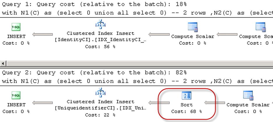
Figure 6-3. Inserting data into the tables: Execution plans
As you can see, there is another sort operator in the case of the index on the uniqueidentifier column. SQL Server sorts randomly generated uniqueidentifier values before the insert, which decreases the performance of the query.
Let’s insert another batch of rows in the table and check index fragmentation. The code for doing this is shown in Listing 6-5. Figure 6-4 shows the results of the queries.
Listing 6-5. Uniqueidentifiers: Inserting rows and checking fragmentation
;with N1(C) as (select 0 union all select 0) -- 2 rows
,N2(C) as (select 0 from N1 as T1 CROSS JOIN N1 as T2) -- 4 rows
,N3(C) as (select 0 from N2 as T1 CROSS JOIN N2 as T2) -- 16 rows
,N4(C) as (select 0 from N3 as T1 CROSS JOIN N3 as T2) -- 256 rows
,N5(C) as (select 0 from N4 as T1 CROSS JOIN N4 as T2) -- 65,536 rows
,IDs(ID) as (select row_number() over (order by (select NULL)) from N5)
insert into dbo.IdentityCI(Val)
        select ID from IDs;

;with N1(C) as (select 0 union all select 0) -- 2 rows
,N2(C) as (select 0 from N1 as T1 CROSS JOIN N1 as T2) -- 4 rows
,N3(C) as (select 0 from N2 as T1 CROSS JOIN N2 as T2) -- 16 rows
,N4(C) as (select 0 from N3 as T1 CROSS JOIN N3 as T2) -- 256 rows
,N5(C) as (select 0 from N4 as T1 CROSS JOIN N4 as T2) -- 65,536 rows
,IDs(ID) as (select row_number() over (order by (select NULL)) from N5)
insert into dbo.UniqueidentifierCI(Val)
        select ID from IDs;

select page_count, avg_page_space_used_in_percent, avg_fragmentation_in_percent
from sys.dm_db_index_physical_stats
(db_id(),object_id(N'dbo.IdentityCI'),1,null,'DETAILED'),

select page_count, avg_page_space_used_in_percent, avg_fragmentation_in_percent
from sys.dm_db_index_physical_stats
(db_id(),object_id(N'dbo.UniqueidentifierCI'),1,null,'DETAILED')
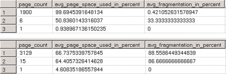
Figure 6-4. Fragmentation of the indexes
As you can see, the index on the uniqueidentifier column is heavily fragmented, and it uses about 40 percent more data pages as compared to the index on the identity column.
A batch insert into the index on the uniqueidentifier column inserts data at different places in the data file, which leads to heavy, random physical I/O in the case of the large tables. This can significantly decrease the performance of the operation.
PERSONAL EXPERIENCE
Some time ago, I had been involved in the optimization of a system that had a large 250GB table with one clustered and three nonclustered indexes. One of the nonclustered indexes was the index on the uniqueidentifier column. By removing this index, we were able to speed up a batch insert of 50,000 rows, from 45 to down 7 seconds.
There are two common use-cases to create indexes on uniqueidentifier columns. The first one is for supporting the uniqueness of values across multiple databases. Think about a distributed system where rows can be inserted into every database. Developers often use uniqueidentifiers to make sure that every key value is unique system wide.
As an alternative solution, you may consider creating a composite index with two columns (InstallationId, Unique_Id_Within_Installation). The combination of those two columns guarantees uniqueness across multiple installations and databases, similar to that of uniqueidentifiers. You can use integer identity or sequence to generate Unique_Id_Within_Installation value, which will reduce the fragmentation of the index.
In cases where a composite index is not desirable, you can create a system-wide unique value by using a byte-mask on the bigint column. High four bytes can be used as InstallationId. Low four bytes can be used as Unique_Id_Within_Installation value.
Another common use-case is security, where uniqueidentifier is used as a security token or a random object id. One possible improvement in this scenario is creating a calculated column using the CHECKSUM() function, indexing it afterwards without creating the index on uniqueidentifier column. The code is shown in Listing 6-6.
Listing 6-6. Using CHECKSUM(): Table structure
create table dbo.Articles
(
        ArticleId int not null identity(1,1),
        ExternalId uniqueidentifier not null
                constraint DEF_Articles_ExternalId
                default newid(),
        ExternalIdCheckSum as checksum(ExternalId),
        /* Other Columns */
);

create unique clustered index IDX_Articles_ArticleId
on dbo.Articles(ArticleId);

create nonclustered index IDX_Articles_ExternalIdCheckSum
on dbo.Articles(ExternalIdCheckSum);
![]() Tip You do not need to persist a calculated column in order to index it.
Tip You do not need to persist a calculated column in order to index it.
Even though the IDX_Articles_ExternalIdCheckSum index is going to be heavily fragmented, it will be more compact as compared to the index on the uniqueidentifier column (a 4 bytes key versus 16 bytes). It also improves the performance of batch operations because of faster sorting, which also requires less memory to proceed.
One thing that you must keep in mind is that the result of the CHECKSUM() function is not guaranteed to be unique. You should include both predicates to the queries as shown in Listing 6-7.
Listing 6-7. Using CHECKSUM(): Selecting data
select ArticleId /* Other Columns */
from dbo.Articles
where checksum(@ExternalId) = ExternalIdCheckSum and ExternalId = @ExternalId
![]() Tip You can use the same technique in cases where you need to index string columns larger than 900 bytes, which is the maximum size of a nonclustered index key. Even though the index on the calculated column would not support range scan operations, it could be used for singleton lookups.
Tip You can use the same technique in cases where you need to index string columns larger than 900 bytes, which is the maximum size of a nonclustered index key. Even though the index on the calculated column would not support range scan operations, it could be used for singleton lookups.
Indexes on uniqueidentifier columns generated with the NEWSEQUENTIALID() function are similar to indexes on identity and sequence columns. They are generally ever-increasing, even though SQL Server resets their base value from time to time.
Using NEWSEQUENTIALID(), however, defeats the randomness of the values. It is possible to guess the next value returned by that function, and you should not use it when security is a concern.
Nonclustered Indexes Design Considerations
It is hard to find the tipping point when joining multiple nonclustered indexes is more efficient than single nonclustered index seek and key lookup operations. When index selectivity is high and SQL Server estimates a small number of rows returned by the Index Seek operation, the Key Lookup cost would be relatively low. In such cases, there is no reason to use another nonclustered index. Alternatively, when index selectivity is low, Index Seek returns a large number of rows and SQL Server would not use it because it is not efficient.
Let’s look at an example where we will create a table and populate it with 1,048,576 rows. Col1 column stores 50 different values in the column, Col2 stores 150 values, and Col3 stores 200 values respectively. Finally, we will create three different nonclustered indexes on the table. The code for doing this is shown in Listing 6-8.
Listing 6-8. Multiple nonclustered indexes: Table creation
create table dbo.IndexIntersection
(
        Id int not null,
        Placeholder char(100),
        Col1 int not null,
        Col2 int not null,
        Col3 int not null
);

create unique clustered index IDX_IndexIntersection_ID
on dbo.IndexIntersection(ID);

;with N1(C) as (select 0 union all select 0) -- 2 rows
,N2(C) as (select 0 from N1 as T1 CROSS JOIN N1 as T2) -- 4 rows
,N3(C) as (select 0 from N2 as T1 CROSS JOIN N2 as T2) -- 16 rows
,N4(C) as (select 0 from N3 as T1 CROSS JOIN N3 as T2) -- 256 rows
,N5(C) as (select 0 from N4 as T1 CROSS JOIN N4 as T2) -- 65,536 rows
,N6(C) as (select 0 from N3 as T1 CROSS JOIN N5 as T2) -- 1,048,576 rows
,IDs(ID) as (select row_number() over (order by (select NULL)) from N6)
insert into dbo.IndexIntersection(ID, Col1, Col2, Col3)
        select ID, ID % 50, ID % 150, ID % 200
        from IDs;

create nonclustered index IDX_IndexIntersection_Col1
on dbo.IndexIntersection(Col1);
create nonclustered index IDX_IndexIntersection_Col2
on dbo.IndexIntersection(Col2);
create nonclustered index IDX_IndexIntersection_Col3
on dbo.IndexIntersection(Col3);
For the next step, let’s look at the execution plan of the query that selects data from the table using three predicates in the where clause. Each predicate can use an Index Seek operation on an individual index. The code for doing this is shown in Listing 6-9 and the execution plan is shown in Figure 6-5.
Listing 6-9. Multiple nonclustered indexes: Selecting data
select ID
from dbo.IndexIntersection
where Col1 = 42 and Col2 = 43 and Col3 = 44;
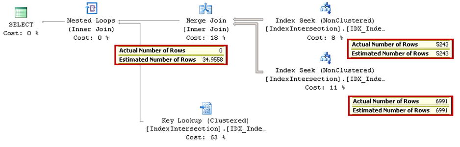
Figure 6-5. Multiple nonclustered indexes: Execution plan with index intersection
There are a couple things worth mentioning here. Even though there is another nonclustered index on Col1, and all indexes include an ID column, which we are selecting, SQL Server elects to use Key Lookup rather than perform a third Index Seek operation. There are 20,971 rows in the table with Col1=42, which makes Key Lookup the better choice.
Another important factor is the cardinality estimation. Even though SQL Server correctly estimates cardinality for both Index Seek operations, the estimation after the join operator is incorrect. SQL Server does not have any data about the correlation of column values in the table, which can lead to cardinality estimation errors and, potentially, suboptimal execution plans.
Let’s add another covering index, which will include all three columns from the where clause, and run the query from Listing 6-9 again. The code creates the index shown in Listing 6-10. The execution plan is shown in Figure 6-6.
Listing 6-10. Multiple nonclustered indexes: Adding covering index
create nonclustered index IDX_IndexIntersection_Col3_Included
on dbo.IndexIntersection(Col3)
include (Col1, Col2)
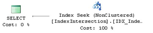
Figure 6-6. Multiple nonclustered indexes: Execution plan with covering index
![]() Note The new index with the two included columns makes the IDX_IndexIntersection_Col1 index redundant. We will discuss this situation later in this chapter.
Note The new index with the two included columns makes the IDX_IndexIntersection_Col1 index redundant. We will discuss this situation later in this chapter.
CPU time and the number of reads are shown in Table 6-2.
Table 6-2. Index intersection vs. covering index
Number of Reads |
CPU Time (ms) |
|
|---|---|---|
Index Intersection |
29 |
9 ms |
Covering Index |
18 |
1 ms |
Even though the number of reads are not very different in both cases, the CPU time of the query with index intersection is much higher than the query with covering index.
The design with multiple narrow nonclustered indexes, which lead to index intersection, can still help, especially in the case of data warehouse systems where queries need to scan and aggregate a large amount of data. They are less efficient, however, when compared to covering indexes. It is usually better to create a small set of wide indexes with multiple columns included rather than a large number of narrow, perhaps single-column indexes.
While ideal indexes would cover the queries, it is not a requirement. A small number of Key Lookup operations is perfectly acceptable. Ideally, SQL Server would perform a nonclustered Index Seek, filtering out rows even further by evaluating other predicates against included columns from the index. This reduces the number of Key Lookups required.
It is impossible to advise you about how many indexes per table you should create. Moreover, it is different for systems with OLTP, Data Warehouse, or mixed workloads. In any case, that number fits into “It Depends” category.
In OLTP systems, where data is highly volatile, you should have the minimally required set of indexes. While it is important to have enough indexes to provide sufficient query performance in the system, you must consider the data modification overhead introduced by them. In some cases, it is preferable to live with suboptimal performance of rarely executed queries, rather than living with the overhead during every data modification operation.
In Data Warehouse environments, you can create a large number of indexes and/or indexed views, especially when data is relatively static and refreshed based on a given schedule. In some cases, you can achieve better update performance by dropping indexes before and recreating them after update.
![]() Note We will cover indexed views in greater detail in Chapter 9, “Views.”
Note We will cover indexed views in greater detail in Chapter 9, “Views.”
Working in mixed-workload environments is always a challenge. I tend to optimize them for OLTP activity, which is usually customer facing and thus more critical. However, you always need to keep reporting/data warehouse aspects in mind when dealing with such systems. It is not uncommon to design a set of tables to store aggregated data, and also use them for reporting and analysis purposes.
Finally, remember to define indexes as unique whenever possible. Unique nonclustered indexes are more compact because they do not store row-id on non-leaf levels. Moreover, uniqueness helps the Query Optimizer to generate more efficient execution plans.
Optimizing and Tuning Indexes
System optimization and performance tuning is an iterative, never-ending process, especially in cases when a system is in development. New features and functions often require you to re-evaluate and refactor the code and change the indexes in the system.
While index tuning is an essential part of system optimization, it is hardly the only area on which you must focus. There are plenty of other factors besides bad or missing indexes that can lead to suboptimal performance. You must analyze the entire stack, which includes the hardware, operating system, SQL Server, and database configurations, when troubleshooting the systems.
![]() Note We will talk about system troubleshooting in greater detail in Chapter 27, “System Troubleshooting.”
Note We will talk about system troubleshooting in greater detail in Chapter 27, “System Troubleshooting.”
Index tuning of existing systems may require a slightly different approach as compared to the development of new systems. With new development, it often makes sense to postpone index tuning until later stages when the database schema and queries are more or less finalized. That approach helps to avoid spending time on optimizations, which become obsolete due to code refactoring. This is especially true in the case of agile development environments, where such refactoring is routinely done at every iteration.
You should still create the minimally required set of the indexes at the very beginning of new development. This includes primary key constraints and indexes and/or constraints to support uniqueness and referential integrity in the system. However, all further index tuning can be postponed until the later development stages.
![]() Note We will talk about constraints in greater detail in Chapter 7, “Constraints.”
Note We will talk about constraints in greater detail in Chapter 7, “Constraints.”
There are two must have elements during index tuning of new systems. First, the database should store enough data, ideally with similar data distribution as that expected in production. Second, you should be able to simulate workload, which helps to pinpoint the most common queries and inefficiencies in the system.
Optimization of existing systems requires a slightly different approach. Obviously, in some cases, you must fix critical production issues, and there is no alternative but to add or adjust indexes quickly. However, as the general rule, you should perform index analysis and consolidation, remove unused and inefficient indexes, and, sometimes, refactor the queries before adding new indexes to the system. Let’s look at all those steps in detail.
Detecting Unused and Inefficient Indexes
Indexes improve performance of read operations. The term read is a bit confusing in the database world, however. Every DML query, such as select, insert, update, delete, or merge reads the data. For example, when you delete a row from a table, SQL Server reads a handful of pages locating that row in every index.
![]() Note Every database system, including the ones with highly volatile data, handles many more reads than writes.
Note Every database system, including the ones with highly volatile data, handles many more reads than writes.
At the same time, indexes introduce overhead during data modifications. Rows need to be inserted into or deleted from every index. Columns must be updated in every index where they are present. Obviously, we want to reduce such overhead and drop indexes that are not used very often.
SQL Server tracks index usage statistics internally and exposes it through sys.dm_db_index_usage_stats and sys.dm_db_index_operation_stats DMOs.
The first data management view-sys.dm_db_index_usage_stats provides information about different types of index operations and the time when such an operation was last performed. Let’s look at an example and create a table, populate it with some data, and look at index usage statistics. The code for doing this is shown in Listing 6-11.
Listing 6-11. Index usage statistics: Table creation
create table dbo.UsageDemo
(
        ID int not null,
        Col1 int not null,
        Col2 int not null,
        Placeholder char(8000) null
);

create unique clustered index IDX_CI
on dbo.UsageDemo(ID);

create unique nonclustered index IDX_NCI1
on dbo.UsageDemo(Col1);

create unique nonclustered index IDX_NCI2
on dbo.UsageDemo(Col2);

;with N1(C) as (select 0 union all select 0) -- 2 rows
,N2(C) as (select 0 from N1 as T1 CROSS JOIN N1 as T2) -- 4 rows
,N3(C) as (select 0 from N2 as T1 CROSS JOIN N2 as T2) -- 16 rows
,IDs(ID) as (select row_number() over (order by (select NULL)) from N3)
insert into dbo.UsageDemo(ID, Col1, Col2)
        select ID, ID, ID
        from IDs;

select
        s.Name + N'.' + t.name as [Table]
        ,i.name as [Index]
        ,ius.user_seeks as [Seeks], ius.user_scans as [Scans]
        ,ius.user_lookups as [Lookups]
        ,ius.user_seeks + ius.user_scans + ius.user_lookups as [Reads]
        ,ius.user_updates as [Updates], ius.last_user_seek as [Last Seek]
        ,ius.last_user_scan as [Last Scan], ius.last_user_lookup as [Last Lookup]
        ,ius.last_user_update as [Last Update]
from
        sys.tables t join sys.indexes i on
                t.object_id = i.object_id
        join sys.schemas s on
                t.schema_id = s.schema_id
        left outer join sys.dm_db_index_usage_stats ius on
                ius.database_id = db_id() and
                ius.object_id = i.object_id and
                ius.index_id = i.index_id
where
        s.name = N'dbo' and t.name = N'UsageDemo'
order by
        s.name, t.name, i.index_id
The User_seeks, user_scans, and user_lookups columns in sys.dm_db_index_usage_stats indicate how many times the index was used for Index Seek, Index Scan, and Key Lookup operations respectively. User_updates indicates the number of inserts, updates, and deletes the index handled. Sys.dm_index_usage_stats DMV also returns statistics about index usage by the system as well as the last time the operation occurred.
As you can see in Figure 6-7, both clustered and nonclustered indexes were updated once, which is the insert statement in our case. Neither of the indexes were used for any type of read activity.

Figure 6-7. Index usage statistics after table creation
One thing worth mentioning is that we are using an outer join in the select. Sys.dm_db_index_usage_stats and sys.dm_index_operation_stats DMO does not return any information about the index if it has not been used since a statistics counters reset.
![]() Important Index usage statistics resets on SQL Server restarts. Moreover, it clears whenever the database is detached or shut down when the AUTO_CLOSE database property is on. Moreover, in SQL Server 2012 and 2014, statistics resets when the index is rebuilt.
Important Index usage statistics resets on SQL Server restarts. Moreover, it clears whenever the database is detached or shut down when the AUTO_CLOSE database property is on. Moreover, in SQL Server 2012 and 2014, statistics resets when the index is rebuilt.
You must keep this behavior in mind during index analysis. It is not uncommon to have indexes to support queries that execute on a given schedule. As an example, you can think about an index that supports a payroll process running on a bi-weekly or monthly basis. Index statistics information could indicate that the index has not been used for reads if SQL Server was recently restarted or, in the case of SQL Server 2012 and 2014, if index was recently rebuilt.
![]() Tip You can consider creating and dropping such an index on the schedule in order to avoid update overhead in between-process executions.
Tip You can consider creating and dropping such an index on the schedule in order to avoid update overhead in between-process executions.
Now let’s run a few queries against the dbo.UsageDemo table, as shown in Listing 6-12.
Listing 6-12. Index usage statistics: Queries
-- Query 1: CI Seek (Singleton lookup)
select Placeholder from dbo.UsageDemo where ID = 5;

-- Query 2: CI Seek (Range Scan)
select count(*)
from dbo.UsageDemo with (index=IDX_CI)
where ID between 2 and 6;

-- Query 3: CI Scan
select count(*) from dbo.UsageDemo with (index=IDX_CI);

-- Query 4: NCI Seek (Singleton lookup + Key Lookup)
select Placeholder from dbo.UsageDemo where Col1 = 5;

-- Query 5: NCI Seek (Range Scan - all data from the table)
select count(*) from dbo.UsageDemo where Col1 > -1;

-- Query 6: NCI Seek (Range Scan + Key Lookup)
select sum(Col2)
from dbo.UsageDemo with (index = IDX_NCI1)
where Col1 between 1 and 5;

-- Queries 7-8: Updates
update dbo.UsageDemo set Col2 = -3 where Col1 = 3
update dbo.UsageDemo set Col2 = -4 where Col1 = 4
If you run select, which displays index usage statistics again, you would see results shown in Figure 6-8.
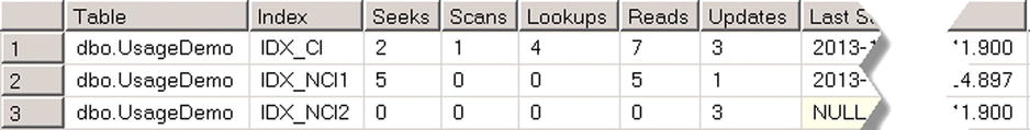
Figure 6-8. Index usage statistics after several queries
There are a couple important things to note here. First, sys.dm_db_index_usage_stats returns how many times queries had corresponding operations in the execution plan, rather than the number of times that operations were executed. For example, there are only four Lookup operations returned for the IDX_CI index, even though SQL Server did Key Lookup for eight rows.
Second, sys.dm_db_index_usage_stats DMV counts both Singleton Lookup and Range Scan as Seek, which corresponds to the Index Seek operator. This could mask the situation when Index Seek performs range scans on a large number of rows. For example, the fifth query in our example scanned all rows from the IDX_NCI1 index although it was counted as Seek rather than Scan.
When you do such an analysis in production systems, you can consider removing indexes, which handle more updates than reads, similar to IDX_NCI2 from our example. In some cases, it is also beneficial not to count scan operations towards reads, especially in OLTP environments, where queries, which perform Index Scan, should be optimized.
While sys.dm_db_index_usage provides a good high-level overview of index usage based on operations from the execution plan, sys.dm_db_index_operation_stats dives deeper and provides detailed level I/O, access methods, and locking statistics for the indexes.
The key difference between two DMOs is how they collect data. Sys.dm_db_index_usage_stats tracks how many times an operation appeared in the execution plan. Alternatively, sys.dm_db_index_operation_stats tracks operations at the row level. In our Key Lookup example, sys.dm_db_index_operation_stats would report eight operations rather than four.
Even though sys.dm_db_index_operation_stats provides very detailed information about index usage, I/O, and locking overhead, it could become overwhelming, especially during the initial performance tuning stage. It is usually easier to do an initial analysis with sys.dm_db_index_usage_stats and use sys.dm_db_index_operation_stats later when fine-tuning the system.
![]() Note You can read more about sys.dm_db_index_operation_stats DMF at Books Online: http://technet.microsoft.com/en-us/library/ms174281.aspx
Note You can read more about sys.dm_db_index_operation_stats DMF at Books Online: http://technet.microsoft.com/en-us/library/ms174281.aspx
![]() Important Make sure that usage statistics collects enough information representing typical system workload before performing an analysis.
Important Make sure that usage statistics collects enough information representing typical system workload before performing an analysis.
Index Consolidation
As we discussed in Chapter 2, “Tables and Indexes: Internal Structure and Access Methods,” SQL Server can use composite index for an Index Seek operation as long as a query has a SARGable predicate on the leftmost query column.
Let’s look at the table shown in Listing 6-13. There are two nonclustered indexes, IDX_Employee_LastName_FirstName and IDX_Employee_LastName, which have a LastName column defined as the leftmost column in the index. The first index, IDX_Employee_LastName_FirstName, can be used for an Index Seek operation as long as there is a SARGable predicate on the LastName column, even when a query does not have a predicate on the FirstName column. Thus the IDX_Employee_LastName index is redundant.
Listing 6-13. Example of redundant indexes
create table dbo.Employee
(
        EmployeeId int not null,
        LastName nvarchar(64) not null,
        FirstName nvarchar(64) not null,
        DateOfBirth date not null,
        Phone varchar(20) null,
        Picture varbinary(max) null
);

create unique clustered index IDX_Employee_EmployeeId
on dbo.Employee(EmployeeId);

create nonclustered index IDX_Employee_LastName_FirstName
on dbo.Employee(LastName, FirstName);

create nonclustered index IDX_Employee_LastName
on dbo.Employee(LastName);
As the general rule, you can remove redundant indexes from the system. Although such indexes can be slightly more efficient during scans due to their compact size, update overhead usually outweighs this benefit.
![]() Note There is always an exception to the rule. Consider a Shopping Cart system, which allows for searching products by part of the name. There are several ways to implement this feature, though when the table is small enough, an Index Scan operation on the nonclustered index on the Name column may provide acceptable performance. In such a scenario, you want to have the index as compact as possible to reduce its size and the number of reads during a scan operation. Thus you can consider keeping a separate nonclustered index on the Name column, even when this index can be consolidated with other ones.
Note There is always an exception to the rule. Consider a Shopping Cart system, which allows for searching products by part of the name. There are several ways to implement this feature, though when the table is small enough, an Index Scan operation on the nonclustered index on the Name column may provide acceptable performance. In such a scenario, you want to have the index as compact as possible to reduce its size and the number of reads during a scan operation. Thus you can consider keeping a separate nonclustered index on the Name column, even when this index can be consolidated with other ones.
The script shown in Listing 6-14 returns information about potentially redundant indexes with the same leftmost column defined. Figure 6-9 shows the result of the execution.
Listing 6-14. Detecting potentially redundant indexes
select
        s.Name + N'.' + t.name as [Table]
        ,i1.index_id as [Index1 ID], i1.name as [Index1 Name]
        ,dupIdx.index_id as [Index2 ID], dupIdx.name as [Index2 Name]
        ,c.name as [Column]
from
        sys.tables t join sys.indexes i1 on
                t.object_id = i1.object_id
        join sys.index_columns ic1 on
                ic1.object_id = i1.object_id and
                ic1.index_id = i1.index_id and
                ic1.index_column_id = 1
        join sys.columns c on
                c.object_id = ic1.object_id and
                c.column_id = ic1.column_id
        join sys.schemas s on
                t.schema_id = s.schema_id
        cross apply
        (
                select i2.index_id, i2.name
                from
                        sys.indexes i2 join sys.index_columns ic2 on
                                ic2.object_id = i2.object_id and
                                ic2.index_id = i2.index_id and
                                ic2.index_column_id = 1
                where
                        i2.object_id = i1.object_id and
                        i2.index_id > i1.index_id and
                        ic2.column_id = ic1.column_id
        ) dupIdx
order by
        s.name, t.name, i1.index_id
![]()
Figure 6-9. Potentially redundant indexes
After you detect potentially redundant indexes, you should analyze all of them on a case-by-case basis. In some cases, consolidation is trivial. For example, if a system has two indexes: IDX1(LastName, FirstName) include (Phone) and IDX2(LastName) include(DateOfBirth), you can consolidate them as IDX3(LastName, FirstName) include(DateOfBirth, Phone).
In the other cases, consolidation requires further analysis. For example, if a system has two indexes: IDX1(OrderDate, WarehouseId) and IDX2(OrderDate, OrderStatus), you have three options. You can consolidate it as IDX3(OrderDate, WarehouseId) include(OrderStatus) or as IDX4(OrderDate, OrderStatus) include(WarehouseId). Finally, you can leave both indexes in place. The decision primarily depends on the selectivity of the leftmost column and index usage statistics.
![]() Tip Sys.dm_db_index_operation_stats function provides information about index usage at the row level. Moreover, it tracks the number of singleton lookups separately from range scans. It is beneficial to use that function when analyzing index consolidation options.
Tip Sys.dm_db_index_operation_stats function provides information about index usage at the row level. Moreover, it tracks the number of singleton lookups separately from range scans. It is beneficial to use that function when analyzing index consolidation options.
Finally, you should remember that the goal of index consolidation is removing redundant and unnecessary indexes. While reducing index update overhead is important, it is safer to keep an unnecessary index rather than dropping a necessary one. You should always err on the side of caution during this process.
Detecting Suboptimal Queries
There are plenty of ways to detect suboptimal queries using both standard SQL Server and third-party tools. There are two main metrics to analyze while detecting suboptimal queries: number of I/O operations and CPU time of the query.
A large number of I/O operations is often a sign of suboptimal or missing indexes, especially in OLTP systems. It also affects query CPU time—the more data that needs to be processed, the more CPU time that needs to be consumed doing it. However, the opposite is not always true. There are plenty of factors besides I/O that can contribute to high CPU time. The most common ones are multi-statement user-defined functions and calculations.
![]() Note We will discuss user-defined functions in more detail in Chapter 10, “Functions.”
Note We will discuss user-defined functions in more detail in Chapter 10, “Functions.”
SQL Profiler is, perhaps, the most commonly used tool to detect suboptimal queries. You can set up a SQL Trace to capture a SQL:Stmt Completed event, and filter it by Reads, CPU, or Duration columns.
There is a difference between CPU time and Duration, however. The CPU column indicates how much CPU time a query uses. The Duration column stores total query execution time. The CPU time could exceed duration in parallel execution plans. High duration, on the other hand, does not necessarily indicate high CPU time, as blocking and I/O latency affect the execution time of the query.
![]() Important Do not use client-side traces with SQL Profiler in a production environment due to the overhead it introduces. Use server-side traces instead.
Important Do not use client-side traces with SQL Profiler in a production environment due to the overhead it introduces. Use server-side traces instead.
Starting with SQL Server 2008, you can use Extended Events instead of SQL Profiler. Extended events are more flexible and introduce less overhead as compared to SQL Traces.
![]() Note We will discuss Extended Events in greater detail in Chapter 28, “Extended Events.”
Note We will discuss Extended Events in greater detail in Chapter 28, “Extended Events.”
SQL Server tracks execution statistics for queries and exposes them via sys.dm_exec_query_stats DMV. Querying this DMV is, perhaps, the easiest way to find the most expensive queries in the system. Listing 6-15 shows an example of a query that returns information about the 50 most expensive queries in a system in terms of average I/O per execution.
Listing 6-15. Using sys.dm_exec_query_stats
select top 50
        substring(qt.text, (qs.statement_start_offset/2)+1,
                ((
                        case qs.statement_end_offset
                                when -1 then datalength(qt.text)
                                else qs.statement_end_offset
                        end - qs.statement_start_offset)/2)+1) as [Sql]
        ,qs.execution_count as [Exec Cnt]
        ,(qs.total_logical_reads + qs.total_logical_writes)
                / qs.execution_count as [Avg IO]
        ,qp.query_plan as [Plan]
        ,qs.total_logical_reads as [Total Reads]
        ,qs.last_logical_reads as [Last Reads]
        ,qs.total_logical_writes as [Total Writes]
        ,qs.last_logical_writes as [Last Writes]
        ,qs.total_worker_time as [Total Worker Time]
        ,qs.last_worker_time as [Last Worker Time]
        ,qs.total_elapsed_time/1000 as [Total Elps Time]
        ,qs.last_elapsed_time/1000 as [Last Elps Time]
        ,qs.creation_time as [Compile Time]
        ,qs.last_execution_time as [Last Exec Time]
from
        sys.dm_exec_query_stats qs with (nolock)
                cross apply sys.dm_exec_sql_text(qs.sql_handle) qt
                cross apply sys.dm_exec_query_plan(qs.plan_handle) qp
order by
        [Avg IO] desc
option (recompile)
The query result, shown in Figure 6-10, helps you quickly find optimization targets in the system. In our example, the second query in the result set executes very often, which makes it an ideal candidate for optimization, even though it is not the most expensive query in the system. Obviously, you can sort the result by other criteria, such as the number of executions, execution time, and so on.
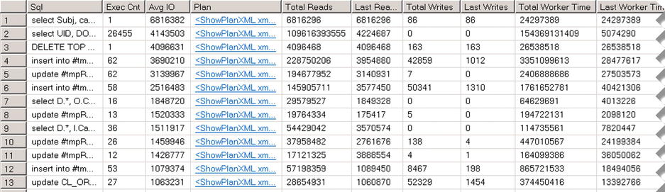
Figure 6-10. Sys.dm_exec_query_stats results
Unfortunately, sys.dm_exec_query_stats returns information only about queries with execution plans cached. As a result, there is no statistics for the statements that use a statement-level recompile with option (recompile). Moreover, execution_count data can be misleading if a query was recently recompiled. You can correlate the execution_count and creation_time columns to detect the most frequently-executed queries.
![]() Note We will discuss Plan Cache in greater detail in Chapter 26, “Plan Caching.”
Note We will discuss Plan Cache in greater detail in Chapter 26, “Plan Caching.”
Starting with SQL Server 2008, there is another DMV sys.dm_exec_procedure_stats, which returns similar information about stored procedures that have execution plans cached. Listing 6-16 shows a query that returns a list of the 50 most expensive procedures in terms of average I/O. Figure 6-11 shows the results of the query on one of the production servers.
Listing 6-16. Using sys.dm_exec_procedure_stats
select top 50
        s.name + '.' + p.name as [Procedure]
        ,qp.query_plan as [Plan]
        ,(ps.total_logical_reads + ps.total_logical_writes) /
                ps.execution_count as [Avg IO]
        ,ps.execution_count as [Exec Cnt]
        ,ps.cached_time as [Cached]
        ,ps.last_execution_time as [Last Exec Time]
        ,ps.total_logical_reads as [Total Reads]
        ,ps.last_logical_reads as [Last Reads]
        ,ps.total_logical_writes as [Total Writes]
        ,ps.last_logical_writes as [Last Writes]
        ,ps.total_worker_time as [Total Worker Time]
        ,ps.last_worker_time as [Last Worker Time]
        ,ps.total_elapsed_time as [Total Elapsed Time]
        ,ps.last_elapsed_time as [Last Elapsed Time]
from
        sys.procedures as p with (nolock) join sys.schemas s with (nolock) on
                p.schema_id = s.schema_id
        join sys.dm_exec_procedure_stats as ps with (nolock) on
                p.object_id = ps.object_id
        outer apply sys.dm_exec_query_plan(ps.plan_handle) qp
order by
        [Avg IO] desc
option  (recompile);

Figure 6-11. Sys.dm_exec_procedure_stats results
SQL Server collects information about missing indexes in the system, and exposes it via a set of DMVs with names starting at sys.dm_db_missing_index. Moreover, you can see suggestions for creating such indexes in the execution plans displayed in Management Studio.
There are two caveats when dealing with suggestions about missing indexes. First, SQL Server suggests the index, which only helps the particular query you are executing. It does not take update overhead, other queries, and existing indexes into consideration. For example, if a table already has an index that covers the query with the exception of one column, SQL Server suggests creating a new index rather than changing an existing one.
Moreover, suggested indexes help to improve the performance of a specific execution plan. SQL Server does not consider indexes that can change the execution plan shape and, for example, use a more efficient join type for the query.
The quality of Database Engine Tuning Advisor (DTA) results greatly depends on the quality of the workload used for analysis. Good and representative workload data leads to decent results, which is much better than suggestions provided by missing indexes DMVs. Make sure to capture the workload, which includes data modification queries in addition to select queries, if you use DTA.
Regardless of the quality of the tools, all of them have the same limitation. They are analyzing and tuning indexes based on existing database schema and code. You can often achieve much better results by performing database schema and code refactoring in addition to index tuning.
Summary
An ideal clustered index is narrow, static, and unique. Moreover, it optimizes most important queries against the table and reduces fragmentation. It is often impossible to design a clustered index that satisfies all of the five design guidelines provided in this chapter. You should analyze the system, business requirements, and workload, and choose the most efficient clustered indexes—even when they violate some of those guidelines.
Ever-increasing clustered indexes usually have low fragmentation because the data is inserted at the end of the table. A good example of such indexes are identities, sequences, and ever-incrementing date/time values. While such indexes may be a good choice for catalog entities with thousands or even millions of rows, you should consider other options in the case of huge tables, with a high rate of inserts.
Uniqueidentifier columns are rarely good candidates for indexes due to their high fragmentation. You should consider implementing composite indexes or byte-masks rather than uniqueidentifiers in these cases when you need to have uniqueness across multiple database servers.
SQL Server rarely uses index intersection, especially in an OLTP environment. It is usually beneficial to have a small set of wide composite nonclustered indexes with included columns rather than a large set of narrow one-column indexes.
In OLTP systems, you should create a minimally required set of indexes to avoid index update overhead. In Data Warehouse systems, the number of indexes greatly depends on the data refresh strategy.
It is important to drop unused and inefficient indexes and perform index consolidation before adding new indexes to the system. This simplifies the optimization process and reduces data modification overhead. SQL Server provides index usage statistics with sys.dm_db_index_usage_stats and sys.dm_db_index_operation_stats DMOs.
You can use SQL Server Profiler, Extended Events, and DMVs, such as sys.dm_exec_query_stats and sys.dm_exec_procedure_stats, to detect inefficient queries. Moreover, there are plenty of tools that can help in monitoring and index tuning. With all that being said, you should always consider query and database schema refactoring as an option. It often leads to much better performance improvements when compared to index tuning by itself.