
8 Validator Tool Suite Filling the Gap between Conventional Software-in-the-Loop and Hardware-in-the-Loop Simulation Environments
Stefan Resmerita, Patricia Derler, Wolfgang Pree and Kenneth Butts
CONTENTS
8.1 Solid System Verification and Validation Needs Improved Simulation Support
8.1.1 Real-Time Behavior in the Validator
8.2 Architecture of a Simulation with the Validator
8.2.1 Basic Features of the Validator
8.3 Setup of a Simulation with the Validator
8.3.1 Target Platform Specification
8.3.2 Task Source Code Annotation
8.4 Embedded System Validation and Verification with the Validator
8.4.1 Simulation with the Validator as the Basis for Advanced Debugging
8.4.2 Simulation with the Validator to Reengineer Legacy Systems
8.1 Solid System Verification and Validation Needs Improved Simulation Support
An embedded system operates in a physical environment with which it interacts through sensors and actuators. An important class of real-time embedded systems is represented by control systems. In this case, the embedded software consists of a set of (controller) tasks and the physical system under control is referred to as the plant. Figure 8.1 sketches the typical architecture of an embedded control system.
Simulation is an approach for testing embedded systems before they are deployed in real-world operation. In simulation, the plant is represented by a software model executed on a host computer, typically a personal computer. In a hardware-in-the-loop (HIL) simulation, the entire embedded system (embedded software consisting of the controller tasks executing on the target platform) is operated in closed loop with the plant model, which is executed in real time on a dedicated computer [1]. Since the embedded software is executed in real time on the target platform, HIL simulations can be used to verify the real-time properties of the embedded system. Thus, any difference between the behavior of the embedded system in a HIL simulation and the corresponding behavior in the real world is due to the abstractions made in plant modeling.
In a software-in-the-loop (SIL) simulation, the embedded software consisting of the controller tasks is executed on a host computer other than the target platform, in closed loop with the plant model. Both simulations (of the controller and the plant model) are typically executed on the same host computer. The SIL model of an embedded system contains the embedded software and an abstraction of the target platform. This abstraction determines how close the software execution in the SIL simulation is to the HIL simulation, provided that the same plant model is used. It ranges from a minimal representation of the target platform that enables only testing of functional (transformational or processing) properties of the software, to full-fledged hardware simulators (called instruction set simulators, ISS), which lead to system behavior close to a HIL simulation, while offering better observability of software executions. Pure functional simulations are fast, but do not allow the testing of timing properties of the embedded system. ISS can be used for timing analysis [2], but they are extremely slow and expensive. Figure 8.2* summarizes the characteristics of conventional SIL, ISS-based SIL, and HIL simulations.
Figure 8.3 summarizes the features and the advantages and disadvantages of state-of-the-art SIL and HIL simulations in comparison with a Validator simulation. Note that the Validator replaces the ISS-based simulation.
Figure 8.4 refines the comparison between the Validator and SIL/HIL approaches. The Validator unifies characteristics of both a SIL and a HIL simulation. The Validator has the flavor of a SIL simulation as it does not require a target platform for executing the embedded software. On the other hand, the Validator separates the simulation of plant and controller tasks as in a HIL simulation.
* Parts of the picture are taken from http://www.mathworks.com/products/xpctarget/ and are courtesy of MathWorks.

FIGURE 8.1 Typical architecture of an embedded system.
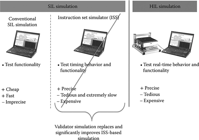
FIGURE 8.2 Conventional software-in-the-loop, instruction set simulators-based software-in-the-loop, and hardware-in-the-loop simulations.
8.1.1 Real-Time Behavior in the Validator
An important aspect is the simulation of real-time behavior. A simple example that illustrates in which respect the Validator is better than typical SIL simulation tools is shown in Figure 8.5. Consider three concurrent tasks, called DynamicsController (DC), MotorController (MC), and ParkingController (PC), that communicate through a shared (global) variable called angle. The code of the tasks is sketched in Figure 8.5a. The tasks DC and MC are periodic with periods equal to 5 and 1 ms, respectively. The task PC is event-triggered. Assume that they are deployed on a real-time operating system with fixed priority preemptive scheduling, where the priorities of the periodic tasks are assigned by a rate monotonic policy. Thus, the MC task has a higher priority than the DC task. Moreover, consider that the PC task has highest priority.
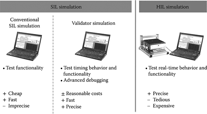
FIGURE 8.3 Validator: advanced software-in-the-loop simulation in between conventional software-in-the-loop and hardware-in-the-loop simulations.
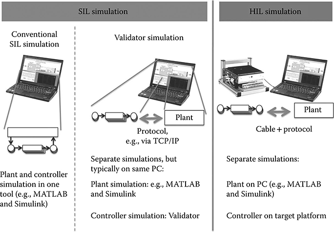
FIGURE 8.4 Structure of a simulation with the Validator.
A snapshot of real-time behavior of the application is depicted in Figure 8.5b, which indicates the sequence of accesses to the variable angle by the three tasks. Note that task DC is triggered first, at 5 ms, and then it is preempted by MC at 6 ms, before writing into the variable angle. Thus, MC reads from angle first. Thereafter, DC resumes and writes the angle, then it is preempted by PC, which reads the variable. Figure 8.5c shows the behavior of the application in a pure functional simulation, where each function is completely executed at the triggering time. In other words, the code is executed in logically zero time. Such a simulation can be obtained in Simulink® [3], for example, by importing the C code as so-called S-function(s) in Simulink. Figure 8.5d presents a timed-functional simulation, where each task has a specified execution time and sharing of processor time among tasks in the system is also simulated. A timed-functional model includes a scheduling component to decide when a triggered task obtains access to the processor. When the task is started, its code is still executed in zero time, thus using the inputs available at that moment; however, the outputs of the task are made available after the specified execution time has elapsed. Examples of SIL simulation environments that offer task-level timed simulation are the Timed Multitasking Ptolemy domain [4] and TrueTime [5]. Notice that the order in which the three tasks access the variable angle is different in the two simulations compared to the real-time case.
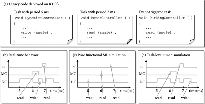
FIGURE 8.5 Examples of mismatch between simulated and real-time behaviors.
On the other hand, a simulation with the Validator would reflect the same order of accesses as in the real-time behavior shown in Figure 8.5b. This requires a detailed execution time analysis and a corresponding instrumentation of the embedded software by the Validator support tools as described in Section 8.3.2.
8.2 Architecture of a Simulation with the Validator
Remember that a simulation with the Validator is a closed-loop co-simulation of the plant under control and the controller tasks. Currently, the Validator supports continuous-time plant models in MATLAB® [6] and Simulink. For that purpose, a communication interface was implemented as a MATLAB and Simulink S-function (see Figure 8.6). The underlying protocol for communication between the plant and the simulation with the Validator is TCP/IP. So both simulations can execute in parallel on the same computer or on different cores or, for example, for efficiency reasons, on different computers. We will extend the Validator to support co-simulation with other simulation environments in the future. For that purpose, communication interfaces must be implemented for the particular simulation environment.
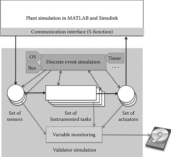
FIGURE 8.6 Architecture of a closed-loop simulation with the Validator.
The Validator also offers a file reader for processing time-stamped values of input data from recorded signals. This is useful for regression testing as discussed in Section 8.4.2.
The Validator simulation engine is a discrete event simulation that takes the platform specifications into account. The platform specifications comprising the operating system (OS), the communication bus, hardware timers, etc. are plug-ins of the Validator simulation engine. The lower half of Figure 8.6 sketches this aspect of the architecture of a Validator simulation. The discrete event simulation controls which of the tasks are executed once the control flow gets back to the discrete event simulation from a task execution. For example, based on the scheduling strategy used by the OS, a higher priority task must interrupt one with a lower priority. In such a situation, the discrete event simulation will switch the execution to the appropriate task. Dashed arrows express this control flow between the instrumented tasks and the discrete event simulation in Figure 8.6. In an analogous way, the Validator takes care of the appropriate reading of sensor values and writing of actuator values.
Figure 8.7 illustrates the discrete event simulation in the Validator in more detail. As the discrete event simulation of the controller tasks proceeds from what we call a spot (S) within a task to the next spot, the control flow between tasks and the discrete event simulation constantly switches back and forth. In the sample scenario in Figure 8.7, the discrete event simulation starts executing sampleTask(). This task executes till it reaches the first spot and returns control to the discrete event simulation. Based on the platform specification, the discrete event simulation decides to interrupt sampleTask() and to give control to anotherTask(), for example, because that one was triggered for execution and has higher priority than sampleTask(). As anotherTask() has only one spot at the end, it executes completely and then returns the control back to the discrete event simulation. Now the discrete event simulation gives back control to sampleTask(). The discrete event simulation continues with the execution of sampleTask() also at the other two spots.

FIGURE 8.7 Sample switching between tasks at spots (S).
8.2.1 Basic Features of the Validator
Let us conclude this overview of the architecture and some core simulation concepts by summarizing the features that result from a bare-bones setup of the Validator:
Variable monitoring. The Validator allows the logging of the time-stamped values of selected variables (global variables and variables local to tasks) to a file. The variable monitor in Figure 8.6 corresponds to that functionality.
Stop and restart simulation runs. The Validator allows stopping a simulation and saving the state of the overall simulation, that is, the simulations of both the plant and the controller tasks. A simulation can later be restarted from a saved state.
8.3 Setup of a Simulation with the Validator
The current version of the Validator basically supports the co-simulation of a plant represented as a variable-step model in MATLAB and Simulink with the controller software written in C. As an advanced feature for reengineering existing controller tasks or adding controller tasks, these tasks can be modeled in MATLAB and Simulink and the Validator then simulates the behavior of both the existing unchanged tasks and the modified or new controller tasks. The only constraint is that the modified or new controller tasks are modeled with discrete time semantics in MATLAB and Simulink. Let us now focus on the typical use case, that is, the co-simulation of a plant represented as variable-step model in MATLAB and Simulink with the controller software written in C.
8.3.1 Target Platform Specification
For an accurate simulation of the controller tasks on a virtual platform, the Validator must have configuration information about the target platform, which is provided by setting properties of the corresponding model components. To specify this information, we use Ptolemy’s front end, as the original research prototype of the Validator was implemented harnessing Ptolemy’s discrete event simulation. The screenshot in Figure 8.8 exemplifies the specification of the behavior of an interrupt service routine (ISR).
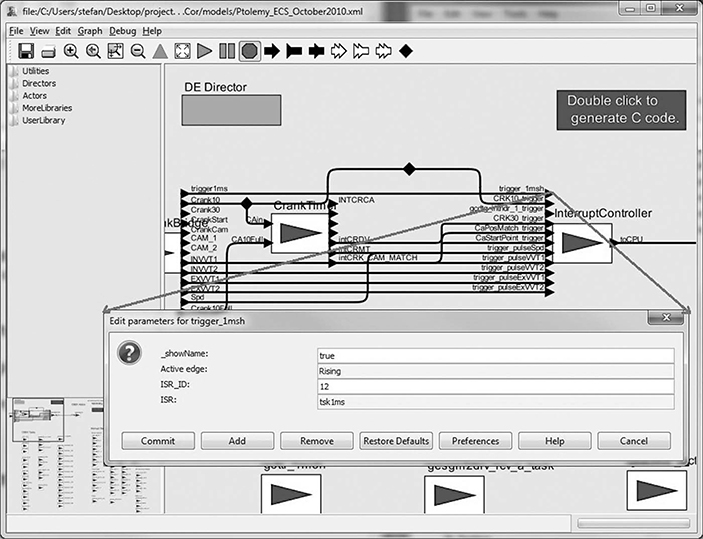
FIGURE 8.8 Specification of interrupt service routine behavior with the Ptolemy front end.
An ISR is represented as a so-called actor in Ptolemy. The actor-oriented programming model is in essence a dataflow-based programming model in which data flows from actor to actor. When activated, each actor performs its specific data processing. An actor-oriented environment such as Ptolemy must account for the execution order of actors. The Validator library, which is used to specify the target platform, comprises various kinds of actors:
Hardware actors model functionality and timing of common hardware parts such as interrupt controllers, timers, bus controllers, hardware sensors, and hardware actuators.
Operating system actors, which implement the functionality of the operating system on the target platform, including scheduling, resource management, and communication between tasks. Currently, the Validator provides actors for the OSEK operating system.
Note that actors are best understood as plug-ins to the discrete event simulation of the Validator, providing the various platform details.
8.3.2 Task Source Code Annotation
In addition to specifying the target platform, the source code of the controller tasks must be instrumented with callbacks to the simulation in the Validator. Details on which aspects require a callback is available in other work [7]. All the spots in the source code are instrumented with callbacks. An example of a type of spot is access to global variables. Between each pair of spots, the execution time must be determined. This is another crucial aspect of target platform information that the Validator must have to achieve its accuracy. From the Validator user point of view, it is only relevant that both the instrumentation and execution time estimation can be automated. Overall, a preparation of the controller tasks for a simulation with the Validator involves the following steps:
Execution time analysis of the application code. This is performed with existing program analysis tools such as AbsInt’s Advanced Analyzer (a3) tool [8]. To increase the accuracy of the estimates, generally details about the architecture of the execution platform must be made available to such tools.
Instrumentation of the code with execution time information.
Instrumentation with callbacks to pass control to the Validator simulation engine for the execution of the tasks.
Generation of what we call the Validator interface code between the Validator simulation engine and the tasks.
In the Validator, these steps are mostly automated by a tool set that achieves a straightforward preparation process. Nevertheless, this automation requires information about the hardware/software architecture, such as the list of lines of code where global variables are accessed.
8.4 Embedded System Validation and Verification with the Validator
This section describes two principal usage scenarios where the Validator excels compared to the state-of-the-art SIL and HIL simulations: advanced debugging of embedded systems and the incremental reengineering of existing embedded systems, including regression testing. Case studies illustrate each particular usage scenario of the Validator.
8.4.1 Simulation with the Validator as the Basis for Advanced Debugging
The key feature of the Validator that allows advanced debugging is that at every source code line in the controller tasks, the overall simulation, that is, of both the controller tasks and the plant, can be stopped. Then variables can be inspected and modified, external code can be executed, etc. Any C debugger can be attached to the Validator to perform the common debugging activities on the controller tasks. A state-of-the-art HIL simulation environment does not offer debugging capabilities. On the other hand, the impreciseness of the state-of-the-art SIL environments makes debugging unattractive or at least less helpful. The accuracy of a Validator simulation makes debugging a valuable means for the validation and verification of embedded systems. Figure 8.9 shows the schematic attachment of a debugger to the Validator. The jet fighter picture represents the plant model.
The screenshot in Figure 8.10 shows a sample set of controller tasks in Eclipse with the gnu debugger (gdb) plugin. The screenshot is discussed in more detail below. We have used gdb as it also supports reverse (or historical) debugging. This allows the following advanced debugging: Once you have turned on reverse debugging, the debugger records all state changes. So if the debugger stops execution at a breakpoint, you cannot only step forward as usual, but also step backward from that point in the code. For example, you want to find the cause of why an actuator value exceeds a certain limit. In this case you would set a conditional breakpoint where the actuator value is set. When the condition holds, the execution stops there and you can step back step by step.
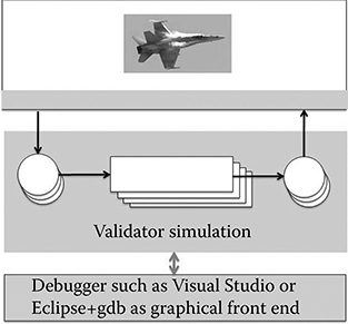
FIGURE 8.9 Attaching a debugger to the Validator.
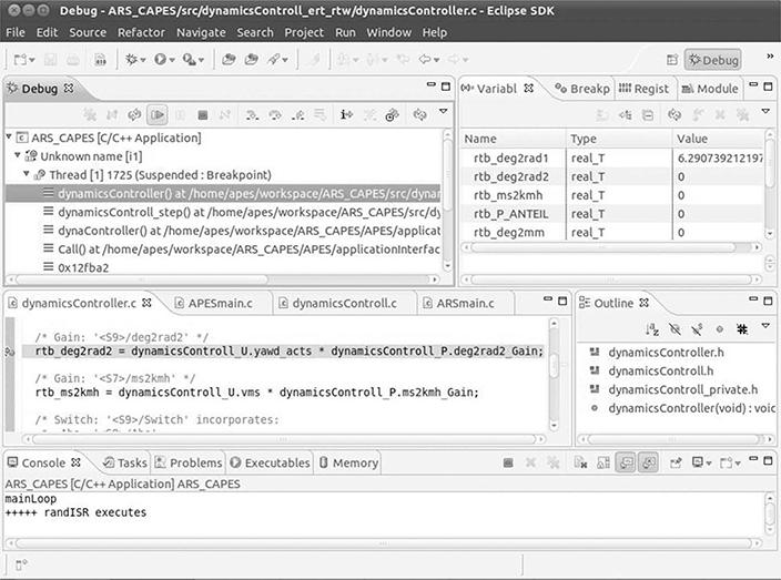
FIGURE 8.10 Start of a sample debugging session in Eclipse with the gnu debugger plugin.
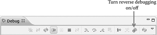
FIGURE 8.11 gnu debugger controls before activating reverse debugging.
The following sequence of screenshots illustrates reverse debugging from a developer’s point of view, with Eclipse and gdb as the graphical front end of the Validator.
In the state shown in Figure 8.10, we just entered the debugging mode by pressing the debug button (the bug in the menu bar on the top left side of the overall window). The execution stopped at an unconditional breakpoint in file dynamicsController.c. The statement at the breakpoint is an assignment statement in which the value of a variable called rtb_deg2rad2 is set. The line is highlighted in the tab labeled dynamicsController.c. According to the subwindow in the top right part of the window, the value of rtb_deg2rad2 is zero.
As a next step, we turn reverse debugging on by pressing the corresponding icon-button (see Figure 8.11). When stepping forward, the debug control panel changes to reflect the feature of reverse debugging, that is, being able to step forward and backward (see Figure 8.12).

FIGURE 8.12 gnu debugger controls for stepping forward and backward.
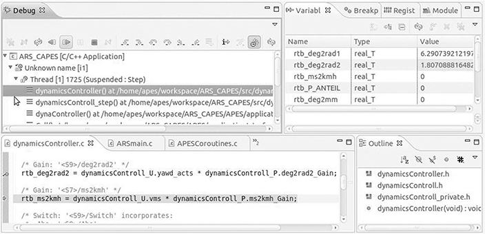
FIGURE 8.13 A step forward.

FIGURE 8.14 A step back.
Let us assume we just stepped forward one statement (see Figure 8.13). The assignment statement where we had originally stopped at the breakpoint has apparently changed the value of variable rtb_deg2rad2 from zero to approximately 1.807.
We can now press the button to go back one step in the debugging process. Figure 8.14 shows the result, that is, as expected, the value of variable rtb_deg2rad2 is again zero. Note that the discrete event simulation of the Validator was implemented such that reverse debugging also functions across multiple tasks. For example, if you have turned on reverse debugging, step forward, and the task is interrupted by another task, that is, the simulation switches to another task, you can still step back up to the point where you started reverse debugging.
As a future extension to the Validator, we will add the feature to also be able to set breakpoints in the plant simulation that halt the overall simulation.
8.4.2 Simulation with the Validator to Reengineer Legacy Systems
The initial motivation for developing the Validator was to provide solid support for the incremental migration of the Engine Controller System (ECS) of a large automotive manufacturer to a version in which the timing behavior is explicitly modeled with the Timing Definition Language (TDL) [9,10]. For that purpose, the behavior of the legacy ECS and the TDL-based ECS should be compared in detail in a SIL simulation, that is, as close to the behavior on the actual platform as possible. Figure 8.15 shows the generic setup for this kind of regression testing by means of the ECS example. The Validator can simulate both versions in parallel.
Note that the ECS comprises millions of lines of code, mostly written in C, and runs on top of an OSEK operating system. This required an efficient implementation of the discrete event simulation of the Validator and an efficient co-simulation with the automobile engine (=plant) model. The engine model is represented in MATLAB and Simulink. To accurately capture the times of the crank angle events, the engine model is simulated with a variable step solver.
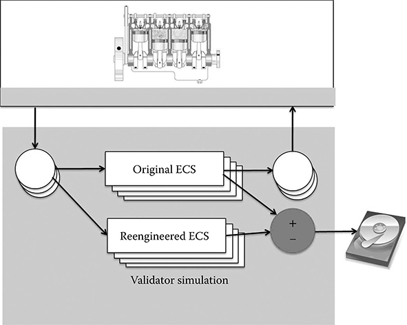
FIGURE 8.15 Regression testing with the Validator.
Implementation of the TDL semantics in the reengineered ECS [9] required a dedicated TDL component called TDL-Machine to be executed every 0.5 ms from the task with highest priority in the system. The TDL-Machine used additional global variables to store and restore values of original global variables at certain points in time.
The highest priority task in the original ECS had a period of 1 ms. To avoid introducing a new task, it was decided to change the original task to have a period of 0.5 ms, to call the TDL-Machine at every task invocation, and to execute the original task code every second invocation. Thus, the execution period of the original code was unaffected.
8.4.2.1 Sample Analysis
Let us take a look at one of the results of the regression tests: Figure 8.16 shows a selection of three signals monitored during a simulation of the two ECS versions with the Validator. Signals S1 and S2 are similar in the two versions. One can notice some delays introduced in the modified version by the execution times of the TDL-Machine. Signal S3 differs significantly towards the end of the simulated time frame.
The cause of the difference could be found by an investigation of task execution profiles. Task execution profile plots are shown in Figures 8.17a through c. In each plot, every task is assigned an identification number (ID). The execution state of a task with ID i is represented by a signal with y-coordinates between i and i + 0.6. A level of i + 0.6 indicates the execution mode E, a level of i + 0.4 means preempted mode P, a level of i + 0.2 indicates the waiting mode W, and a level of i means the task is in the suspended mode S. The plot in Figure 8.17a is obtained from the simulation of the original software, the plot in Figure 8.17b is obtained from the simulation of the software with the TDL-Machine and its execution time, and the plot in Figure 8.17c corresponds to the simulation of the software with the TDL-Machine but without its execution time. In case of Figure 8.17c, the TDL-Machine was executed in simulation, but its execution time was set to zero, for the purpose of debugging.
The ID of the highest priority task is 8. In the simulation represented by the plot in Figure 8.17a, the execution time of this task at time instant 5 is approximately 0.05 ms. In the simulation of the plot in Figure 8.17b, the same execution requires about 0.20 ms. In Figure 8.17c, the same task execution takes about 0.17 ms. It follows that the main difference between the executions in Figures 8.17a and 8.17b is not given by the execution time of the TDL-Machine, but it is because the different state of the hardware platform resulted from the execution of the TDL function. Since the TDL-Machine performs many accesses to new memory locations, the main difference occurs most probably in the cache state. If the delays in the signals in the new version are not acceptable, then one should focus on minimizing the effect of the TDL-Machine on the platform state rather than on minimizing the execution time of the function code. For example, the TDL-Machine could be changed to operate only on local variables, or additional variables used by this function could be stored in the processor’s internal memory space.
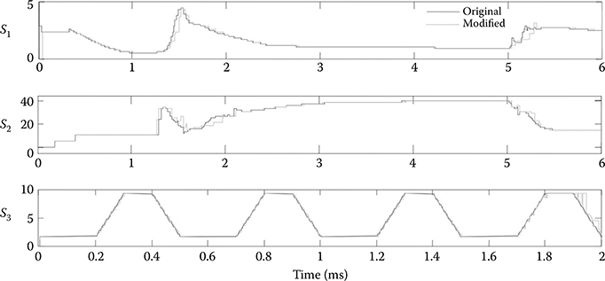
FIGURE 8.16 Comparison of three signals.
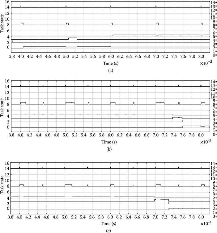
FIGURE 8.17 (a) Original ECS. (b) ECS with additional functionality. (c) ECS with additional functionality whose execution time is set to zero.
8.5 Related Work
This section groups existing work in the area of simulation of embedded applications into two categories, related to the main features of the Validator: the ability to synchronize with an external plant model for closed-loop simulation (co-simulation) and the special focus on legacy software and its execution time.
8.5.1 Co-Simulation
The main purpose of co-simulation is validating the functionality of hardware (HW) and software (SW) components by simulating two or more system parts that are described on different levels of abstraction. The challenge is the interface between the different abstraction levels. A simulation of the system should be possible throughout the entire design process where the model of the same component is refined iteratively [11]. Co-simulation as a basis for co-design and system verification can be performed in various manners where typically a trade-off between accuracy and performance must be made [12]. Various commercial and academic co-simulation frameworks have been proposed in literature; surveys can be found in Edwards et al. [12], Huebert [13], and Bosman [14].
In HW/SW co-simulation, the processor model is responsible for connecting hardware and software models. The processor can be modeled at gate level, which is the most accurate but also the slowest solution, with clock cycle accuracy or on an instruction-set level. Faster co-simulation tools do not model the processor but implement a synchronization handshake [15]. Some co-simulation environments also provide a virtual operating system to emulate or simulate the hardware [16].
Many approaches use ISS to obtain correct timing information. However, ISS are slow because of the fine granularity of the simulation. Performance issues are addressed for instance with caching [17] and distributed simulation by applying distributed event-driven simulation techniques.
The co-simulation framework used by the Validator does not provide a model of the central processor unit and does not employ an ISS because of performance reasons. We work with execution time at the source code level. Hardware components are modeled at a higher level of abstraction. The simulation tool was in an original prototype implemented based on Ptolemy. Another Ptolemy-based co-simulation approach can be found in Liu et al. [17].
8.5.2 Modeling and Simulating Legacy Code
There are various approaches that generate models from legacy code, but only a few of them include the timing aspect in the modeling. Some software reverse engineering efforts take the software and find equivalent modeling constructs in a modeling language to reconstruct the same behavior as exhibited by the software. An example is provided in Sangiovanni-Vincentelli [18], where C programs are reverse-engineered to Simulink models. This, however, usually leads to complex models that are not understandable and thus do not aid in gaining new insights in the embedded software system.
Code instrumentation and delaying of task execution to obtain a certain behavior is used by Wang et al. [19]. In this approach, the authors employ code instrumentation to generate deadlock-free code for multicore architectures. Timed Petri nets are generated from (legacy) code by instrumenting the code at points where locks to shared resources are accessed to model blocking behavior of software. A controller is synthesized from the code and used at runtime to ensure deadlock-free behavior of the software on multicore platforms by delaying task executions that would lead to deadlocks. The objective of the Validator is different: to replicate the real-time behavior of a given application (within certain accuracy limits). Thus, the Validator does not alter the functional behavior of the application.
In Sifakis et al. [20], a formal framework is described for building timed models of real-time systems to verify functional and timing correctness. Software and environment models are considered to operate in different timing domains that are carefully related at input and output operations. A timed automaton of the software is created by annotating code with execution time information. The tool presented in that work restricts the control part of task implementations and the plant model to Esterel programs. The authors state that for tasks written in general purpose languages such as C, an analysis must reveal observable states and computation steps. The Validator provides such an analysis and can be used for application code written in C and environment models in Matlab and Simulink.
The benefits of modeling all aspects of an embedded system at a suitable level of abstraction are well known and have been addressed in the platform-based design approach. Tools such as Metropolis [21] offer a framework for platform-based design where functionality and platform concerns are specified independently. A mapping between functionality and a given platform must be provided. Representation of components and the mapping between functional and architectural networks is possible at different levels of refinement. The purpose of Metropolis is to support the top-down design process. All system components are modeled in an abstract specification language, which is parsed to an abstract syntax tree and provided to back-end tools for analysis and simulation. Although Metropolis allows the inclusion of legacy components, its main goal is not a bottom-up analysis of legacy systems but a top-down specification of the required behavior and a specification of the platform. In the approach presented here, the behavior of the components such as the data flow or temporal constraints is retrieved from simulation. As opposed to Metropolis, we do not require a specification of the functionality in a metamodel language, which is further translated into SystemC [22] for simulation. Our approach directly includes the software as simulation components. Simulation tools related to the Validator are TrueTime [5] from academia and the commercial tool ChronSim from INCHRON [23]. Compared to these tools, the Validator offers a series of advanced features, as described in the chapter.
8.6 Conclusions
The Validator is tool suite for significantly improved SIL verification and validation of real-time embedded applications. The first prototype was developed with Ptolemy and was originally called the Access Point Event Simulator (APES). Chrona [24] developed the Validator as a product out of APES. Chrona’s Validator has evolved to a product version that scales to the simulation of real-world embedded software consisting of millions of lines of code. The Validator achieves time-functional simulation of application software and execution platform in closed loop with a plant model. The Validator works independently of a specific domain as long as a simulation model for a particular plant is available.
A simulation with the Validator is based on a systematic manner to instrument the application code with execution time information and execution control statements, which enables capturing real-time behavior at a finer and more appropriate time granularity than most of the currently available similar tools. Chrona’s Validator is able to simulate preemption at the highest level of abstraction that still allows for capturing the effect of preemption on data values, avoiding at the same time the slow, detailed simulation achieved by instruction set simulators. Moreover, the Validator can operate in closed loop with plant models simulated by a different tool. Also, Chrona’s Validator enables traversing preemption points during forward and reverse debugging of the application. In the Validator, one can start a simulation from a previously saved state. Being implemented entirely in C, the Validator can be easily interfaced or even integrated with existing simulation tools such as MATLAB and Simulink.
Acknowledgments
We would like to thank Edward Lee (University of California, Berkeley) for valuable insights during numerous discussions of the Validator concepts and his support in implementing an earlier prototype of the Validator with Ptolemy II.
References
1. Mosterman, Pieter J., Sameer Prabhu, and Tom Erkkinen. 2004. “An Industrial Embedded Control System Design Process.” In Proceedings of the Inaugural CDEN Design Conference (CDEN’04), pp. 02B6-1 through 02B6-11, July 29–30. Montreal, Quebec, Canada.
2. Krause, Matthias, Dominik Englert, Oliver Bringmann, and Wolfgang Rosenstiel. 2008. “Combination of Instruction Set Simulation and Abstract RTOS Model Execution for Fast and Accurate Target Software Evaluation.” In Proceedings of the 6th IEEE/ACM/ IFIP International Conference on Hardware/Software Codesign and System Synthesis (CODES+ISSS ‘08), 143–48. New York: ACM.
3. MathWorks®. Simulink® 7.5 (R2010a). http://www.mathworks.com/products/simulink/. Accessed on September 10, 2010.
4. Liu, Jie, and Edward Lee. 2002. “Timed Multitasking for Real-Time Embedded Software.” IEEE Control Systems Magazine 23: 65–75.
5. Cervin, Anton, Dan Henriksson, Bo Lincoln, Johan Eker, and Karl-Erik Årzén. June 2003. “How Does Control Timing Affect Performance? Analysis and Simulation of Timing Using Jitterbug and TrueTime.” IEEE Control Systems Magazine 23 (3): 16–30.
6. MathWorks®. Matlab® 7.10 (R2010a). http://www.mathworks.com/products/matlab/. Accessed on September 10, 2012.
7. Resmerita, Stefan, and Patricia Derler. May 2011. “Wolfgang Pree: Validator—Concepts and Their Implementation.” Technical Report, University of Salzburg.
8. AbsInt. 2011. aiT Worst-Case Execution Time Analyzer. http://www.absint.com/ait/. Accessed on July 12, 2010.
9. Resmerita, Stefan, Kenneth Butts, Patricia Derler, Andreas Naderlinger, and Wolfgang Pree. 2011. “Migration of Legacy Software Towards Correct-by-Construction Timing Behavior.” In Monterey Workshops 2010, edited by R. Calinescu and E. Jackson, LNCS 6662, pp. 55–76. Springer Verlag, Heildelberg.
10. Templ, Josef, Andreas Naderlinger, Patricia Derler, Peter Hintenaus, Wolfgang Pree, and Stefan Resmerita. 2012. “Modeling and Simulation of Timing Behavior with the Timing Definition Language (TDL).” In Real-time Simulation Technologies: Principles, Methodologies, and Applications, edited by K. Popovici and P. Mosterman (this volume), pp. 157–176, Boca Raton, FL: CRC Press.
11. Kalavade, Asawaree P. 1995. “System-Level Codesign of Mixed Hardware-Software Systems.” PhD thesis, University of California, Berkeley, Chair-Lee, Edward A.
12. Edwards, Stephen, Luciano Lavagno, Edward A. Lee, and Alberto Sangiovanni-Vincentelli. 1999. “Design of Embedded Systems: Formal Models, Validation, and Synthesis.” In Proceedings of the IEEE, 366–90. IEEE, Washington, DC.
13. Huebert, Heiko. June 1998. “A Survey of HW/SW Cosimulation Techniques and Tools.” Master’s thesis, Royal Institute of Technology, Stockholm, Sweden.
14. Bosman, G. 2003. “A Survey of Co-design Ideas and Methodologies.” Master’s thesis, Vrije Universiteit, Amsterdam.
15. Mentor Graphics Corporation. 1996–1998. “Seamless Co-verification Environment User’s and Reference Manual, V 2.2.” Wilsonville, Oregon.
16. Saha, Indranil Saha, Kuntal Chakraborty, Suman Roy, B. VishnuVardhan Reddy, Venkatappaiah Kurapati, and Vishesh Sharma. 2009. “An Approach to Reverse Engineering of C Programs to Simulink Models with Conformance Testing.” In ISEC ’09: Proceedings of the 2nd India Software Engineering Conference, pp. 137–8. New York: ACM.
17. Liu, Jie, Marcello Lajolo, and Alberto Sangiovanni-Vincentelli. 1998. “Software Timing Analysis Using HW/SW Cosimulation and Instruction Set Simulator.” In CODES/ CASHE ’98: Proceedings of the 6th International Workshop on Hardware/Software Codesign, pp. 65–9. Washington, DC: IEEE Computer Society.
18. Sangiovanni-Vincentelli, Alberto. February 2002. “Defining Platform-Based Design.” EEDesign of EE Times.
19. Wang, Yin, Stephane Lafortune, Terence Kelly, Manjunath Kudlur, and Scott Mahlke. 2009. “The Theory of Deadlock Avoidance via Discrete Control.” In POPL ’09: Proceedings of the 36th Annual ACM SIGPLAN-SIGACT Symposium on Principles of Programming Languages, pp. 252–63. New York: ACM.
20. Sifakis, Joseph, Stavros Tripakis, and Sergio Yovine. January 2003. “Building Models of Real-Time Systems from Application Software.” Proceedings of the IEEE 91 (1): 100–11.
21. Balarin, Felice, Massimiliano D’Angelo, Abhijit Davare, Douglas Densmore, Trevor Meyerowitz, Roberto Passerone, and Alessandro Pinto, et al. January 2009. “Platform-Based Design and Frameworks: Metropolis and Metro II.” In Model-Based Design of Heterogeneous Embedded Systems, edited by G. Nicolescu and P. Mosterman. Boca Raton, FL: CRC Press.
22. Ghenassia, Frank. 2006. Transaction-Level Modeling with Systemc: Tlm Concepts and Applications for Embedded Systems. Secaucus, NJ: Springer-Verlag New York, Inc.
23. Inchron. 2011. The Chronsim Simulator. http://www.inchron.com/chronsim.html. Accessed on September 10, 2010.
24. Chrona’s Validator tool suite. 2011. http://www.CHRONA.com. Accessed on September 10, 2010.