Chapter 16 Concurrent Simulation for Online Optimization of Discrete Event Systems

The path to fast and accurate computer simulation depends on the objective one pursues. In the case of offline applications, the goal is typically to simulate a highly complex system to study its behavior in detail and to ascertain its performance. An example might involve the design of an expensive large-scale system to be built, in which case it is essential to use simulation for the purpose of exploring whether it meets performance specifications and cost constraints under alternative designs and control mechanisms. In such a realm, reasonably fast simulation time is desirable but not indispensable, and one may be more likely to trade off execution speed for higher fidelity. On the contrary, for online applications, we often refer to real-time simulation as a tool for generating efficient models providing predictive capability while an actual system is operating as well as the means to explore alternatives that may be implemented in real time. An example might arise when a system is about to operate in an environment it was never originally designed for; one is then interested in simulating how the system would behave in such an environment, possibly under various implementable alternatives (e.g., adding resources to it or modifying the parametric settings of a controller). On the basis of the results, one might proceed in the new setting, abort, or choose the best possible modification before proceeding. In such cases, obtaining information fast from simulation is not just desirable, but an absolute requirement.

Speeding up the process of information extraction from simulation may be attained in various ways. First, one can use abstraction to replace a detailed model by a less detailed one that is still sufficiently accurate to provide useful information in a real-time frame for making decisions such as choosing between two or more alternatives to be implemented. Another approach is to use multiple processors operating in parallel. This is usually referred to as distributed simulation, where different parts of the entire simulation code are assigned to different processors. By operating in parallel, N such processors have the potential of reducing the time to complete a simulation run by a factor of N. However, this is rarely feasible since the execution must be synchronized. Thus, one slow processor may delay the rest either because its output is necessary for them to continue execution or because of inefficiencies in the way the code was distributed. Nonetheless, this approach enables interoperability as well as allowing for geographic distribution of processors and some degree of fault tolerance.^1,2

The goal of concurrent simulation is to provide, at the completion of a single run, information that would normally require M separate simulation runs and to do so with minimal overhead. Thus, suppose that the goal of a real-time simulation application is to determine how a given performance measure J(θ) varies as a function of some parameter θ in the absence of any analytical expression for J(θ). This requires the generation of a simulation run at least once for every value of θ of interest. It is easy to see how demanding this process becomes: if θ represents options from a discrete set {θ₁, … , θ_M}, we need M simulation runs under each of θ₁, … , θ_M. It is even more demanding when the system is stochastic, requiring a large number of simulation runs under a fixed θ_i to achieve desired levels of statistical accuracy. Concurrent simulation techniques are designed to accomplish the task of providing estimates of all J(θ₁), … , J(θ_M) at the end of a single simulation run instead of M runs. Moreover, if a simulation run under some θ_i requires T time units, then instead of M · T total simulation time, a concurrent simulation algorithm is intended to deliver all M estimates in T + τ_M time units where often τ_M < T and certainly T + τ_M << M · T. In general, θ = [θ¹, … , θ^N] is a vector of parameters, in which case concurrent simulation is applied to each element θⁱ over all M ⁱ values of θⁱ that are of interest. Thus, at the end of a single simulation run, we obtain estimates of $J (θ_{1}^{i}), \dots, J (θ_{M^{i}}^{i})$ $J (θ_{1}^{i}), \dots, J (θ_{M^{i}}^{i})$ for all i = 1,…, N at the same time. To keep notation manageable, however, in most of the discussion that follows we consider a scalar θ.

It is important to emphasize the difference between distributed and concurrent simulation. In distributed simulation, the code for a single simulation run is shared over M processors. Thus, at the end of the run, a single set of input–output data (equivalently, one estimate of the relationship J(θ)) is obtained. In concurrent simulation, a single processor simulates a system but also concurrently simulates it under M − 1 additional settings. Thus, at the end of the run, we obtain a total of M input–output data (equivalently, estimates of J(θ₁), … , J(θ_M)). If, in addition, M processors are available for concurrent simulation, then the speedup resulting from the concurrent construction is further increased by naturally assigning a processor to each of the M threads estimating J(θ_i) for each i = 1, … , M. The speedup benefit in concurrent simulation comes not from the presence of extra processing capacity (which also implies a higher cost) but from the efficient sharing of input data over multiple simulations of the same system under different settings. Another way of interpreting it is as a method that addresses the question “What if a given system operating under a nominal value θ₁ were to operate under θ₂, … , θ_M with the same input conditions?” The answer to these M − 1 “what if” questions can be obtained without having to reproduce M − 1 distinct simulations by “brute force”; instead, it can be deduced by processing data from the nominal simulation so as to track the differences caused by replacing θ₁ by θ_i, i = 2, … , M. In Monte Carlo simulation for instance, the computational cost of generating random variates from several distributions is much higher than the cost of performing this difference tracking and constructing state trajectories under multiple settings captured by θ₁, … , θ_M.

In this chapter, we will first review the formalism and theoretical foundations of concurrent simulation as it applies to the class of discrete event systems (DES), also developed in the works by Cassandras and Lafortune³ and Cassandras and Panayiotou.⁴ The state space of a typical DES involves at least some discrete components, giving rise to piecewise constant state trajectories. This can be exploited to predict changes in an observed state trajectory under some setting θ_i when the system operates under θ_j ≠ θ_i. Formally, this is studied as a general sample path constructability problem. In particular, given a DES sample path under a parameter value θ, the problem is to construct multiple sample paths of the system under different values using only information available along the given sample path. A solution to this problem can be obtained when the system under consideration satisfies a constructability condition. Unfortunately, this condition is not easily satisfied. However, it is possible to enforce it at some expense. For a large class of DES modeled as Markov chains, there are two techniques known as the Standard Clock (SC) method and the Augmented System Analysis (ASA), which provide solutions to the constructability problem. In a more general setting (where one cannot impose any assumptions on the stochastic characteristics of the event processes), we will describe the process through which the problem is solved by coupling an observed sample path to multiple concurrently generated sample paths under different settings. This ultimately leads to a detailed procedure known as the Time Warping Algorithm (TWA).

At this point, it is worth emphasizing that concurrent sample path constructability techniques can be used in two different modes. First, they can be used offline to obtain estimates of the system performance under different parameters θ₁, … , θ_M from a single simulation run under θ₀. A main objective in this case is to reduce the overall simulation time to achieve high speedup. This approach was investigated in the work by Cassandras and Panayiotou.⁴ The emphasis of this chapter is on the online use of sample path constructability techniques where the nominal sample path θ₀ is simply the one observed during the operation of the actual system. In this case, based on the observed data, the goal is to estimate the system’s performance again under a set of hypothetical parameter values θ₁, … , θ_M. In this case, a controller can monitor the performance of the system under the different parameters J(θ₀), … , J(θ_M), and at the end of each epoch, it can switch to the parameter that achieves the best performance. In this setting, another important advantage of concurrent sample path constructability techniques is that they use common random numbers (CRN), and as a result, the probability of selecting the parameter that optimizes the performance J(θ) is increased. Another important advantage of the online use of concurrent sample path constructability techniques is that it does not require any prior knowledge of the underlying distributions of the various events since those are already embedded in the occurrence times of the observed events. This makes the approach applicable even when the distributions are time varying.

We begin the chapter by reviewing the Stochastic Timed Automaton (STA) modeling framework for DES in Section 16.2. This is the framework used by most commercial discrete event simulators, thus facilitating the implementation of the concurrent simulation techniques to be described. In Section 16.3, we define the general sample path constructability problem. We also review the SC method and the ASA for DES with Markovian structure in their event processes. Then, in Section 16.4, we describe the procedure through which the general constructability problem is solved and derive the aforementioned TWA. In Section 16.5, we describe how the TWA can be used together with optimization schemes (e.g.,^5–8 to solve dynamic resource allocation problems (see also works by Panayiotou and Cassandras^9,10). The chapter ends with some final thoughts and conclusions.

16.2 Modeling and Simulating Discrete Event Systems

We begin with a DES modeled as an automaton (χ, ε, f, Γ, x₀), where χ is a countable state space, ε is a countable event set, f:χ × ε→χ is a state transition function, Γ:χ→2^ε is the active (or feasible) event function so that Γ(x) is the set of all events e ∈ ε for which f(x, e) is defined, and it is called the active event set (or feasible event set), and finally, x₀ is the initial state. The automaton is easily modified to (χ, ε, Γ, x₀, p, p₀) to include probabilistic state transition mechanisms: the state transition probability p(x′; x, e′) is defined for all x, x′ ∈ χ, e′ ∈ ε and is such that p(x′; x, e′) = 0 for all e′ ∉ Γ(x); in addition, p₀(x) is the probability mass function (pmf) P [x₀ = x], x ∈ χ, of the initial state x₀. For simplicity, we assume that the DES satisfies the “noninterruption condition,” that is, once an event is enabled, it cannot be disabled; however, this is not essential to the rest of our discussion.

This model is referred to as an untimed automaton,³ since it provides no information as to which among all events feasible at some state x will occur next. To resolve this issue, we define a clock structure associated with an event set ε (which we will hencefoth assume finite with cardinality N) to be a set V = {V₁, … , V_N} of event life-time sequences V_i = {v_i_,1, v_i_,2, …}, one for each event i ∈ ε, with v_i_,k ∈ ℝ⁺. This leads to the definition of a timed automaton (χ, ε, f, Γ, x₀, V), where V is a clock structure, and (χ, ε, f, Γ, x₀) is an (untimed) automaton. The timed automaton generates a state sequence

x^{'} = f (x, e^{'}) (16.1)

$x^{'} = f (x, e^{'}) (16.1)$

driven by an event sequence {e₁, e₂, …} generated through

e^{'} = \arg \min_{i \in Γ (x)} {y_{i}} (16.2)

$e^{'} = \arg \min_{i \in Γ (x)} {y_{i}} (16.2)$

with the clock values y_i, i ∈ ε, defined by

{y^{'}}_{i} = {\begin{cases} y_{i} - y * i f i \neq e^{'} and i \in Γ (x^{'}) \\ v_{i, N_{i + 1}} if i = e^{'} or i \notin Γ (x) \end{cases} i \in Γ (x^{'}) (16.3)

${y^{'}}_{i} = {\begin{cases} y_{i} - y * i f i \neq e^{'} and i \in Γ (x^{'}) \\ v_{i, N_{i + 1}} if i = e^{'} or i \notin Γ (x) \end{cases} i \in Γ (x^{'}) (16.3)$

where the interevent time y^* is defined as

y * = \min_{i \in Γ (x)} {y_{i}} (16.4)

$y * = \min_{i \in Γ (x)} {y_{i}} (16.4)$

and the event scores N_i, i ∈ ε, are defined by

{N^{'}}_{i} = {\begin{cases} N_{i + 1} if i = e^{'} i \notin Γ (x) \\ N_{i} otherwise \end{cases} i \in Γ (x^{'}) (16.5)

${N^{'}}_{i} = {\begin{cases} N_{i + 1} if i = e^{'} i \notin Γ (x) \\ N_{i} otherwise \end{cases} i \in Γ (x^{'}) (16.5)$

In addition, initial conditions are y_i = v_i_,1 and N_i = 1 for all i ∈ Γ(x₀). If i ∉ Γ(x₀), then y_i is undefined and N_i = 0.

Note that this is precisely how a discrete event simulator generates state trajectories of DES using the event lifetime sequences V_i = {v_i_,1, v_i_,2, …} as input. The simulator maintains the Clock, the State x, and the Event Calendar where all feasible events at state x along with their clock values are maintained. The entries of the Event Calendar are ordered so as to determine y^* through Equation 16.4 and hence determine the “triggering event” e′ in Equation 16.2. Once this is accomplished, the simulator updates the State through Equation 16.1 and the Clock by setting its new value to

t^{'} = t + y * (16.6)

$t^{'} = t + y * (16.6)$

Then, since x′ is available, Γ(x′) is determined, and all Clock values for i ∈ Γ(x′) are updated through Equation 16.3. This results in an updated Event Calendar and the process repeats. It is important to note that this state trajectory construction is entirely event driven and not time driven. In other words, it is the Event Calendar that determines the next State of the system as well as the next value of the Clock. If the Event Calendar ever becomes empty, the process cannot continue, a situation that we often identify as a “deadlock” in the system. This event-driven mechanism is to be contrasted to a time-driven approach where the clock is updated through t′ = t + ∆, where ∆ is a fixed time step. This is clearly inefficient, since often there is a large interval between the current event and the next event; during this interval, the simulator needlessly updates the clock. What is worse, however, is that one or more events may in fact occur within an interval [t, t + ∆] in which case such a time-driven procedure fails to update the state until t + ∆. To counteract that, one might use a smaller value of ∆, which in turn forces more needless clock updates.

The final step is to incorporate randomness into a timed automaton by allowing the elements of an event lifetime sequence to be random variables. Furthermore, in a more general setting, the state transition mechanisms can be assumed probabilistic. Thus, we define a stochastic clock structure associated with an event set ε to be a set of distribution functions G = {G_i: i ∈ ε} characterizing the stochastic clock sequences. This leads to the definition of a STA (ε, χ, Γ, p, p₀, G), where (ε, χ, Γ, p, p₀) is an automaton with a probabilistic state transition mechanism and G is a stochastic clock structure. The STA generates a stochastic state sequence {X₀, X₁, …} (i.e., a sample path) through a transition mechanism (based on observations X = x, E′ = e′):

X^{'} = x^{'} with probability p (x^{'}; x, e^{'})

$X^{'} = x^{'} with probability p (x^{'}; x, e^{'})$

and it is driven by a stochastic event sequence {E₁, E₂, …} generated through the same process as Equations 16.2 through 16.5 with E replacing e, Y_i replacing y_i, and V_i_,k replacing v_i_,k. In addition,

{V_{i, k}} ~ G_{i}

${V_{i, k}} ~ G_{i}$

where the tilde (∼) notation denotes “with distribution” and initial conditions are X₀ ∼ p₀(x), and Y_i = V_i_,1 and N_i = 1 if i ∈ Γ(X₀). If i ∉ Γ(X₀), Y_i is undefined and N_i = 0. For simplicity, for the remainder of the chapter, we will assume a STA with deterministic state transition functions (ε, χ, f, Γ, G) where the source of randomness is the stochastic nature of event lifetimes.

Example

To illustrate the definition of a STA, let us apply it to a simple single-server queueing system with a sequence of arriving tasks waiting in a First-In-First-Out (FIFO) queue with infinite capacity. This is normally written as “G/G/1,” where the first two Gs denote the probability distribution characterizing the arrival process and the service process, respectively: the letter G stands for “General” to indicate that neither distribution is assumed known. The number 1 indicates that there is a single server processing arriving task requests. In this case, we set χ = {0, 1, …} to be the state space, so that x ∈ χ is the number of tasks in the system (including one in process), and ε = {a, d} to denote an arrival and a departure event, respectively. Clearly, Γ(x) = {a, d} for all x ∈ χ except for Γ(0) = {a}, since a departure from an empty system is infeasible. Since all state transitions are deterministic, we revert to the usual state transition mechanism x′ = f(x, e′), and we have x′ = x + 1 if e′ = a and x′ = x − 1 if e′ = d and x > 0.

A G/G/1/K queueing system is one where the queueing capacity is limited to K tasks. In this case, the model above is modified so that χ = {0, 1, … , K} and x' = x + 1 if e' = a, x < K, while x' = x if e' = a, x = K. If, in addition, there is some information regarding the distribution functions of the arrival and service processes, then these are specified through stochastic clock structure G = {G_a, G_d}. For example, if the arrival process is Poisson with rate λ, we have G_a(t) = 1 − e⁻λ^t, t ≥ 0 with G_a(t) = 0 for t < 0, and if the service process is uniformly distributed over [0, 1], we have G_d(t) = t for t ∈ [0, 1], G_d(t) = 0 for t < 0, and G_d(t) = 1 for t > 1. In this case, the queueing system is represented by the notation M/U/1/K.

16.3 Sample Path Constructability

Let us consider a DES modeled as a STA and let Θ = {θ₀, θ₁, … , θ_M} be a finite set containing all possible values that a parameter θ in this model may take. As mentioned earlier, in general, θ is a vector, so if θ = [θ¹, … , θ^N] and θⁱ can take Mⁱ values, then we can write $Θ = {θ_{1}^{1}, \dots, θ_{M °}^{1}, \dots, θ_{1}^{N}, \dots, θ_{M^{N}}^{N}}$ $Θ = {θ_{1}^{1}, \dots, θ_{M °}^{1}, \dots, θ_{1}^{N}, \dots, θ_{M^{N}}^{N}}$ Moreover, it is possible that Θ is a set of feasible operating policies or design choices that affect the dynamics of the DES. For example, in a G/G/1/θ queueing system, we may consider the capacity θ as a model parameter taking integer values for some set Θ = {1, … , K}. Alternatively, we may want to study the performance of this DES as a function of different queueing disciplines such as FIFO, Last-In-First-Out (LIFO), and Random; in this case, Θ = {FIFO, LIFO, Random}. Yet another example is the simultaneous investigation of the queue capacity and the queueing discipline, and in this case, Θ₃ = Θ₁ × Θ₂ Let J(θ) denote a performance metric of the system under θ. Since the DES is in general stochastic, let

ω (θ) = {(e_{k}, t_{k}), k = 1, 2, \dots}

$ω (θ) = {(e_{k}, t_{k}), k = 1, 2, \dots}$

be a sample path of the system when it is operating under θ, where e_k ∈ ε is the kth event observed in this sample path and t_k is the associated occurrence time. The corresponding sample performance metric is denoted by L[ω(θ)], and we are interested in estimating performance metrics of the form

J (θ) = E [L [ω (θ)]]

$J (θ) = E [L [ω (θ)]]$

Our premise is that there is no closed-form expression for J(θ); therefore, we rely on simulation to obtain sample paths ω(θ) from which we can compute L[ω(θ)] and ultimately estimate the expected value E[L[ω(θ)]], typically through

\hat{J} (θ) = \frac{1}{R} \sum_{i = 1}^{R} L [ω_{i} (θ)]

$\hat{J} (θ) = \frac{1}{R} \sum_{i = 1}^{R} L [ω_{i} (θ)]$

where ω_i(θ) is the ith sample path (equivalently, simulation run or, for online applications, a finite length observation interval). In applications where the objective is to select the value of θ in = {θ₀, θ₁, … , θ_M} that minimizes J(θ), then the “brute force” trial-and-error approach involves a total of (M + 1) · R simulation runs to estimate performance for each of the M + 1 settings and then select the optimal one. For offline optimization, assuming all event lifetime distributions are known, then this is feasible, although possibly computationally expensive. For online applications, however, where event lifetime distributions may not be known exactly or where event lifetime distributions may be time varying, the brute force approach is infeasible. The goal of concurrent simulation methods is to extract estimates $\hat{J} (θ_{i}), i = 1, \dots, M$ $\hat{J} (θ_{i}), i = 1, \dots, M$ by observing only one sample path under parameter θ₀. To study whether this is possible and under what conditions, we pose the sample path constructability problem as follows:

For a DES under θ₀, construct all sample paths ω(θ₁), … , ω(θ_M) given a realization of lifetime sequences V₁, … , V_N and the sample path ω(θ₀).

Images

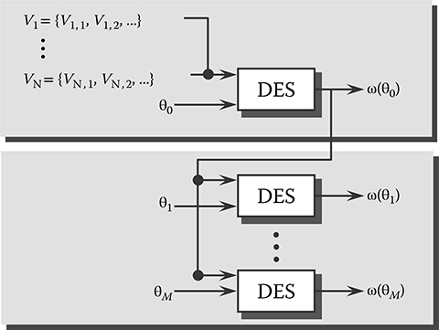
FIGURE 16.1 The sample path constructability problem.

This is illustrated in Figure 16.1. There is a simple sufficient condition under which the constructability problem can be solved. This condition consists of two parts. First, let {X_k(θ)}, k = 1, 2, … , be the state sequence observed in a sample path ω(θ) under θ in which the lifetime sequences are V_i = {V_i_,1, V_i_,2, …}, i = 1, … , N. We refer to this as the nominal sample path. Then, for θ_m ≠ θ, suppose the DES is driven by the same event sequence generated under θ, giving rise to a new state sequence {X_k(θ_m)}, k = 1, 2, … , and sample path ω(θ_m). We say that ω(θ_m) is observable with respect to ω(θ) if Γ(X_k(θ_m)) ⊆ Γ(X_k(θ)) for all k = 1, 2, … . Thus, we have the following observability condition (OB):

(OB) Let ω(θ) be a sample path under θ, and {X_k(θ)}, k = 0, 1, … , the corresponding state sequence. For θ_m ≠ θ, let ω(θ_m) be the sample path generated by the event sequence in ω(θ). Then, for all k = 0, 1, … , Γ(X_k(θ_m)) ⊆ Γ(X_k(θ)).

By construction, the two sample paths are “coupled” so that the same event sequence drives them both. As the two state sequences subsequently unfold, condition (OB) states that every state observed in the nominal sample path is always “richer” in terms of feasible events. In other words, from the point of view of ω(θ_m), all feasible events required at state X_k(θ_m) are observable in the corresponding state X_k(θ).

The second part of the constructability condition involves the clock values Y_i of events i ∈ ε. Let H(t, z) be the conditional distribution of Y_i defined as follows:

H (t, z) = P [Y_{i} \leq t | V_{i} > z]

$H (t, z) = P [Y_{i} \leq t | V_{i} > z]$

where z is the observed age of the event at the time H(t, z) is evaluated (i.e., the time elapsed since event i was last triggered). Given the lifetime distribution G_i(t), and since V_i = Y_i + z, we have

H (t, z) = P [V_{i} \leq z + t | V_{i} > z] = \frac{G_{i} (z + t) - G_{i} (z)}{1 - G_{i} (z)}

$H (t, z) = P [V_{i} \leq z + t | V_{i} > z] = \frac{G_{i} (z + t) - G_{i} (z)}{1 - G_{i} (z)}$

Since both the distribution H(t, z) and the event age generally depend on the parameter θ, we write H(t, z_i_,k(θ); θ) to denote the cumulative distribution function (cdf) of the clock value of event i ∈ ε, given its age z_i_,k(θ). Then, the constructability condition (CO) is as follows:

(CO) Let ω(θ) be a sample path under θ, and {X_k(θ)}, k = 0, 1, … , the corresponding state sequence. For θ_m ≠ θ, let ω(θ_m) be the sample path generated by the event sequence in ω(θ). Then,

Γ (X_{k} (θ_{m})) \subseteq Γ (X_{k} (θ)) for all k = 0, 1, \dots

$Γ (X_{k} (θ_{m})) \subseteq Γ (X_{k} (θ)) for all k = 0, 1, \dots$

and

H (t, z_{i, k} (θ_{m}); θ_{m}) = H (t, z_{i, k} (θ); θ) for all i \in Γ (X_{k} (θ)), k = 0, 1, \dots

$H (t, z_{i, k} (θ_{m}); θ_{m}) = H (t, z_{i, k} (θ); θ) for all i \in Γ (X_{k} (θ)), k = 0, 1, \dots$

The first part is simply (OB), while the second part imposes a requirement on the event clock distributions. Details on (CO) are found in the work by Cassandras and Lafortune,³ but we note here two immediate implications: (1) if the STA has a Poisson clock structure, then (OB) implies (CO), and (2) if Γ(X_k(θ_m)) = Γ(X_k(θ)) for all k = 0, 1, … , then (CO) is satisfied. Clearly, (1) simply follows from the memoryless property of the exponential distribution, and it reduces the test of constructability to the purely structural condition (OB). Regarding (2), it follows from the fact that if feasible event sets are always the same under θ and θ_m, then all event clock values are also the same.

Example

Consider a G/G/1/K queueing system, where K = 1, 2, … is the parameter of interest. Under K = 3, a sample path ω₃ is obtained. We then pose the question whether a sample path ω₂, constructed under K = 2, is observable with respect to ω₃. In what follows, {X_k(K)}, k = 1, 2, … , denotes the state sequence in a sample path generated with queueing capacity K = 1, 2, … . The two state transition diagrams are shown in Figure 16.2. Since condition (OB) must be tested under the assumption that both sample paths are generated by the exact same input, it is convenient to construct a new system whose state consists of the joint queue lengths of the two original systems. This is referred to as an augmented system. As shown in Figure 16.2, we assume both sample paths start from a common state (say 0, for simplicity). On the left part of the augmented system state transition diagram, the two states remain the same. In fact, a difference arises only when (1) X_k(3) = X_k(2) = 2 for some k, and (2) event a occurs. At this point, the state transition gives X_k _{+ 1}(3) = 3, but X_k _{+ 1}(2) = 2. From this point on, the two states satisfy X_k(3) = X_k(2) + 1, as seen in Figure 16.2, until state (1, 0) is visited. At this point, the only feasible event is a departure d, bringing the state back to (0, 0).

By inspection of the augmented system state transition diagram, we see that (OB) is trivially satisfied for the three states such that X_k(3) = X_k(2). It is also easily seen to be satisfied at (3, 2) and (2, 1), since Γ(x) = {a, d} for all x > 0. The only remaining state is (1, 0), where we see that Γ(X_k(2)) = Γ(0) = {a} ⊂ {a, d} = Γ(1) = Γ(X_k(3)), and (OB) is satisfied. Thus, sample paths of this system under K = 2 are indeed observable with respect to sample paths under K = 3.

Images

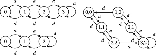
FIGURE 16.2 State transition diagrams for G/G/1/3 and G/G/1/2 along with the corresponding augmented system.

Let us now reverse the roles of the two parameter values and corresponding sample paths. Thus, the question is whether a sample path constructed under K = 3 is observable with respect to a sample path under K = 2. Returning to Figure 16.2, and state (1, 0) in particular, note that Γ(X_k(3)) = Γ(1) = {a, d} ⊃ {a} = Γ(0) = Γ(X_k(2)). Thus, the feasible event d, needed at state X_k(3) = 1 is unobservable at the corresponding state X_k(2) = 0. Therefore, it is interesting to note that condition (OB) is not symmetric with respect to the role of the parameter chosen as the “nominal” one.

As the previous example illustrates, even for DES modeled as Markov chains, condition (CO) is not generally satisfied because (OB) may fail. However, it is possible to enforce (OB) at the expense of some computational cost or the cost of temporarily “suspending” the construction of the sample paths under some values in {θ₁, … , θ_M}. We will review next two methods that accomplish this goal, the SC method and ASA, before addressing the more general question of solving the constructability problem for arbitrary DES.

16.3.1 Standard Clock Approach

The SC approach¹¹ applies to stochastic timed automata with a Poisson clock structure so that all event lifetime distributions are exponential, and we have $G_{i} (t) = 1 - e^{- λ_{i}^{t}}$ $G_{i} (t) = 1 - e^{- λ_{i}^{t}}$ for all i ∈ ε. Thus, every event process in such systems is characterized by a single Poisson parameter λ_i. As already pointed out, the distributional part of (CO) is immediately satisfied by the memoryless property of the exponentially distributed event lifetimes. The observability condition (OB) will be forced to be satisfied by choosing a nominal sample path to simulate such that Γ(x) = ε for all states x. To accomplish this, let

Λ (x) = \sum_{i \in Γ (x)} λ_{i} (16.7)

$Λ (x) = \sum_{i \in Γ (x)} λ_{i} (16.7)$

A property of Markov chains is that the distribution of the triggering event taking place at state x is given by

p_{i} (x) = \frac{λ}{Λ (x)}, i \in Γ (x) (16.8)

$p_{i} (x) = \frac{λ}{Λ (x)}, i \in Γ (x) (16.8)$

Moreover, exploiting the uniformization of Markov chains, we replace Λ(x) by a uniform rate γ ≥ Λ(x) common to all x so that the additional probability flow [γ − Λ(x)] at state x corresponds to “fictitious events” that leave the state unchanged. In our case, we choose this uniform rate to be the maximal rate over all events:

Λ = \sum_{i = ε} λ_{i} (16.9)

$Λ = \sum_{i = ε} λ_{i} (16.9)$

In the uniformized model, every event is always feasible. However, events i such that i ∉ Γ(x) for the original model leave the state unchanged, and they are ignored. Moreover, the mechanism through which the triggering event at any state is determined becomes independent of the state. Specifically, in Equation 16.7, we can now set Λ(x) = Λ for all x. Therefore, the triggering event distribution at any state is simply p_i = λ_i/Λ. The fact that all events are permanently feasible in the uniformized model, combined with the memoryless property of the exponential event lifetime distribution, immediately implies the constructability condition (CO). In short, the way the SC approach gets around the problem of potentially unobservable events is by simulating a system in which all events are forced to occur at all states, and hence satisfy (OB). Although this results in several fictitious events, that is, events i such that i ∉ Γ(x), it also makes for a general-purpose methodology within the realm of Poisson event processes.

There is one additional simplification we can make to this scheme. We can generate all interevent times {V₁, V₂, …} from the cdf G(t) = 1 − e^−t and then rescale any specific V_k through V_k(Λ) = V_k/Λ for any given Λ. This allows us to define all event times: assuming the system starts at time zero, we have t₁ = V₁, t₂ = t₁ + V₂, and so on. The resulting sequence is referred to as the SC and can be generated in advance of any simulation. The specific SC algorithm for constructing sample paths under {θ₀, … , θ_M} concurrently with the simulation of a nominal system constructed in this manner is as follows:

INITIALIZATION: Construct a SC: {V₁, V₂, …}, V_k ∼ 1 − e^–t, t > 0.
FOR EVERY CONSTRUCTED SAMPLE PATH m = 0, 1, … , M:

Determine the triggering event E_m (by sampling from the pmf p_i = λ_i/Λ).
Update the state: X′_m = f_m(X_m, E_m)
Rescale the observed interevent time V: V_m = V/Λ_m. Return to step 1 for the next event.

The SC concurrent simulation scheme is extremely simple and applies to any Markov chain regardless of its state transition mechanism. Its main drawback is that it is not applicable for online applications where some of the rates of the event lifetime distributions are not known a priori since fictitious events are not observable. Futhermore, for offline applications, several of the events generated at step 1 of the algorithm may be wasted in the sense that they are fictitious and cause no change in the state of one or more of the constructed sample paths.

16.3.2 Augmented System Analysis

Unlike the SC method, ASA^12,13 is based on observing a real sample path under some setting θ₀ and accepting the fact that constructability must be satisfied based on whatever events this observed sample path provides. Let ω(θ₀) denote the observed sample path, and we need to check whether we can use information extracted from ω(θ₀) to construct ω(θ_m) for some θ_m ≠ θ₀. As the observed state sequence {X_k(θ₀)} unfolds, we can construct the sequence {X_k(θ_m)} as long as Γ(X_k(θ_m)) ⊆ Γ(X_k(θ₀)). Now, suppose that we encounter a state pair (X(θ₀), X(θ_m)) such that Γ(X(θ_m)) ⊃ Γ(X(θ₀)). This means that there is at least one event, say i ∈ Γ(X(θ_m)), which is unobservable at state X(θ₀). At this point, the construction of ω(θ_m) must be suspended, since the triggering event at state X(θ_m) cannot be determined. Then, the key idea in ASA is the following: keep the state in ω(θ_m) fixed at X(θ_m) and keep on observing ω(θ₀) until some new state X′(θ₀) is entered that satisfies Γ(X(θ_m)) ⊆ Γ(X′(θ₀)). The only remaining question is how long ω(θ_m) must wait in suspension. Note that we do not require “state matching,” that is, we do not require that X′(θ₀) = X(θ_m) to continue the construction, but the weaker condition of “event matching”: Γ(X(θ_m)) ⊆ Γ(X′(θ)).

We will use ℳ_m to denote the mode of ω(θ_m), which can take on either the special value ACTIVE or a value from the state space χ_m. This gives rise to the following Event Matching algorithm:

INITIALIZATION: Set ℳ_m = ACTIVE and X_m = X₀.
WHEN ANY EVENT (say α) IS OBSERVED AND THE STATE IN ω(θ₀)

BECOMES X, FOR m = 1, … , M:

If ℳ_m = ACTIVE, update the state: X′_m= f_m(X_m, α) and if Γ(X′_m) ⊃ Γ(X) (i.e., observability is violated), set ℳ_m = X′_m.
If ℳ_m ≠ ACTIVE and Γ(ℳ_m) ⊆ Γ(X), set ℳ_m = ACTIVE; if ℳ_m ≠ ACTIVE, and Γ(ℳ_m) ⊃ Γ(X), then continue.

In step 2, the condition M_m ≠ ACTIVE and Γ(M_m) ⊆ Γ(X) implies that ω(θ_m) was suspended at the time this event occurs, but since the observability condition Γ(M_m) ⊆ Γ(X) is satisfied, the sample path construction can resume. The validity of the event matching scheme rests on basic properties of Markov processes, which enable us to “cut and paste” segments of a given sample path to produce a new sample path that is stochastically equivalent to the original one (for more details, see the work by Cassandras and Lafortune³). Note that no stopping condition is specified, since this is generally application dependent. Also, as in the case of the SC construction, the result of the Event Matching algorithm is a complete sample path; any desired sample function can subsequently be evaluated from it for the purpose of estimating system performance under all {θ₀, θ₁, … , θ_M} of interest. The main drawback of ASA is the need to suspend a sample path construction for a potentially long time interval. This problem is the counterpart of the drawback we saw for the SC approach, which consists of “wasted random number generations,” however, unlike SC, ASA can construct sample paths under different parameters using information directly observable from the sample path of an actual system. Finally, it is worth pointing out that the Event Matching algorithm can be modified so as to allow for at most one event process that is not Poisson; details of this extension are given in the work by Cassandras and Lafortune.³

16.4 Concurrent Simulation Approach for Arbitrary Event Processes

In this section, we describe a method for solving the constructability problem without having to rely on the Markovian structure of the event processes in the DES model, based on the sample path coupling approach first presented in the work by Cassandras and Panayiotou.⁴ We start by making some assumptions, followed by three subsections. Section 16.4.1 introduces some notation and definitions; Section 16.4.2 presents the Time Warping Algorithm (TWA) for implementing the general solution to the constructability problem; Section 16.4.3 quantifies the speedup realized through the TWA; and Section 16.4.4 discusses extensions resulting from relaxing the assumptions presented next.

The four assumptions that follow simplify our analysis and apply to a large class of DES. However, they can also be eventually relaxed (see the work by Cassandras and Panayiotou⁴).

(A1) Feasibility Assumption: Let x_n be the state of the DES after the occurrence of the nth event. Then, for any n, there exists at least one r > n such that e ∈ Γ(x_r) for any e ∈ ε.

(A2) Invariability Assumption: Let ε be the event set under the nominal parameter θ₀ and let ε_m be the event set under θ_m ≠ θ₀. Then, ε_m = ε.

(A3) Similarity Assumption: Let G_i(θ₀), i ∈ ε be the event lifetime distribution for the event i under θ₀ and let G_i(θ_m), i ∈ ε be the corresponding event lifetime distribution under θ_m. Then, G_i(θ₀) = G_i(θ_m ) for all i ∈ ε.

(A4) State Invariability Assumption: Let G_i(x_k ), i ∈ ε and x_k ∈ χ be the event lifetime distribution of event i if i is activated when the system state is x_k. Then, G_i(x_k ) = G_i(x_l ) for all x_k, x_l ∈ χ and all i ∈ ε.

Assumption A1 guarantees that in the evolution of any sample path, all events in ε will always become feasible at some point in the future. If, for some DES, assumption A1 is not satisfied, that is, there exists an event α that never gets activated after some point in time, then, as we will see, it is possible that the construction of some sample path will remain suspended forever waiting for α to happen. Note that a DES with an irreducible state space immediately satisfies this condition.

Assumption A2 states that changing a parameter from θ₀ to some θ_m ≠ θ₀ does not alter the event set ε. More importantly, A2 guarantees that changing to θ_m does not introduce any new events so that all event lifetimes for all events can be observed from the nominal sample path (the converse, i.e., fewer events in ε_m, would still make it possible to satisfy (OB)).

Assumption A3 guarantees that changing a parameter from θ₀ to some θ_m ≠ θ₀ does not affect the distribution of one or more event lifetime sequences. This allows us to use exactly the same lifetimes that we observe in the nominal sample path to construct the perturbed sample path. In other words, our analysis focuses on structural system parameters rather than distributional parameters. As we will see, however, it is straightforward to handle the latter at the expense of some computational cost.

Finally, assumption A4 guarantees that the observed lifetimes do not depend on the current state of the system. This allows us to use any event lifetime of an event e ∈ ε that has been observed irrespective of the current state of the system and, therefore, to employ “event matching” as opposed to “state matching” when a constructed sample path becomes active after being suspended for violating the (OB) condition.

16.4.1 Notation And Definitions

Let

ξ (n, θ) = {e_{j} : j = 1, \dots, n}

$ξ (n, θ) = {e_{j} : j = 1, \dots, n}$

with e_j ∈ ε, be the sequence of events that constitute an observed sample path ω(θ) up to n total events. Although ξ(n,θ) is clearly a function of the parameter θ, we will write ξ(n) and adopt the notation

\hat{ξ} (k) = {{\hat{e}}_{j} : j = 1, \dots, k}

$\hat{ξ} (k) = {{\hat{e}}_{j} : j = 1, \dots, k}$

for any constructed sample path under a different value of the parameter up to k events in that path. It is important to realize that k is actually a function of n, since the constructed sample path is coupled to the observed sample path through the observed event lifetimes. However, again for the sake of notational simplicity, we will refrain from continuously indicating this dependence.

Next, we define the score of an event i ∈ ε in a sequence ξ(n), denoted by $s_{i}^{n} = [ξ (n)] i$ $s_{i}^{n} = [ξ (n)] i$ , to be the nonnegative integer that counts the number of instances of event i in this sequence. The corresponding score of i in a constructed sample path is denoted by ${\hat{s}}_{i}^{k} = {[\hat{ξ} (k)]}_{i}$ ${\hat{s}}_{i}^{k} = {[\hat{ξ} (k)]}_{i}$ . In what follows, all quantities with the symbol “^” above them refer to a typical constructed sample path.

Associated with every event type i ∈ ε in ξ(n) is a sequence of s_n event lifetimes

V_{i} (n) = {v_{i} (1), \dots, v_{i} (s_{i}^{n})} for all i \in ε

$V_{i} (n) = {v_{i} (1), \dots, v_{i} (s_{i}^{n})} for all i \in ε$

The corresponding set of sequences in the constructed sample path is as follows:

{\hat{V}}_{i} (k) = {v_{i} (1), \dots, v_{i} ({\hat{s}}_{i}^{k})} for all i \in ε

${\hat{V}}_{i} (k) = {v_{i} (1), \dots, v_{i} ({\hat{s}}_{i}^{k})} for all i \in ε$

which is a subsequence of V_i(n) with k ≤ n. In addition, we define the following sequence of lifetimes:

{\tilde{V}}_{i} (n, k) = {v_{i} ({\hat{s}}_{i}^{k} + 1), \dots, v_{i} (s_{i}^{n})} for all i \in ε

${\tilde{V}}_{i} (n, k) = {v_{i} ({\hat{s}}_{i}^{k} + 1), \dots, v_{i} (s_{i}^{n})} for all i \in ε$

which consists of all event lifetimes that are in V_i(n) but not in ${\hat{V}}_{i} (k)$ ${\hat{V}}_{i} (k)$ . Associated with any one of these sequences are the following operations. Given some W_i = {w_i(j),…,w_i(r)},

Suffix Addition: W_i + {w_i(r + 1)} = {w_i(j), … , w_i(r), w_i(r + 1)} and
Prefix Subtraction: W_i − {w_i(j)} = {w_i(j + 1), … , w_i(r)}.

Note that the addition and subtraction operations are defined so that a new element is always added as the last element (the suffix) of a sequence, whereas subtraction always removes the first element (the prefix) of the sequence. At this point, it is worth pointing out that to construct the various event lifetime sequences, it is necessary that the event lifetime sequences are observable from the nominal sample path. For offline approaches, this is generally simple since the lifetimes can be directly recorded from the simulator. For online approaches, this is possible for invertible systems, that is, systems for which event lifetimes can be recovered from the output of a system (i.e., sequence of events, states, and transition epochs) (see the work by Park and Chong¹⁴ for invertibility conditions as well as an appropriate algorithm). Next, define the set

A (n, k) = {i : i \in ε, s_{i}^{n} > {\hat{s}}_{i}^{k}} (16.10)

$A (n, k) = {i : i \in ε, s_{i}^{n} > {\hat{s}}_{i}^{k}} (16.10)$

which is associated with ${\tilde{V}}_{i} (n, k)$ ${\tilde{V}}_{i} (n, k)$ and consists of all events i whose corresponding sequence ${\tilde{V}}_{i} (n, k)$ ${\tilde{V}}_{i} (n, k)$ contains at least one element. Thus, every i ∈ A(n, k) is an event that has been observed in ξ(n) and has at least one lifetime that has yet to be used in the coupled sample path $\hat{ξ} (k)$ $\hat{ξ} (k)$ . Hence, A(n, k) should be thought of as the set of available events to be used in the construction of the coupled path.

Finally, we define the following set, which is crucial in our approach:

M (n, k) = Γ ({\hat{x}}_{k}) - (Γ ({\hat{x}}_{k - 1}) - {{\hat{e}}_{k}}) (16.11)

$M (n, k) = Γ ({\hat{x}}_{k}) - (Γ ({\hat{x}}_{k - 1}) - {{\hat{e}}_{k}}) (16.11)$

where, clearly, M(n, k) ⊆ ε. Note that ${\hat{e}}_{k}$ ${\hat{e}}_{k}$ is the triggering event at the (k − 1)th state visited in the constructed sample path. Thus, M(n, k) contains all the events that are in the feasible event set $Γ ({\hat{x}}_{k})$ $Γ ({\hat{x}}_{k})$ but not in $Γ ({\hat{x}}_{k - 1})$ $Γ ({\hat{x}}_{k - 1})$ ; in addition, ${\hat{e}}_{k}$ ${\hat{e}}_{k}$ also belongs to M(n, k) if it happens that ${\hat{e}}_{k} \in Γ ({\hat{x}}_{k})$ ${\hat{e}}_{k} \in Γ ({\hat{x}}_{k})$ . Intuitively, M(n, k) consists of all missing events from the perspective of the constructed sample path when it enters a new state ${\hat{x}}_{k}$ ${\hat{x}}_{k}$ , that is, those events already in $Γ ({\hat{x}}_{k - 1})$ $Γ ({\hat{x}}_{k - 1})$ that were not the triggering event remain available to be used in the sample path construction as long as they are still feasible. All other events in the set are “missing” as far as residual lifetime information is concerned.

The concurrent sample path construction process we are interested in consists of two coupled processes, each generated by an STA as detailed in Section 16.2, through Equations 16.1 to 16.6. The observed sample path and the one to be constructed both satisfy this set of equations. Our task is to derive an additional set of equations that captures the coupling between them. In particular, our goal is to enable event lifetimes from the observed ξ(n) to be used to construct a sequence $\hat{ξ} (k)$ $\hat{ξ} (k)$ . First, observe that the process described by Equations 16.1 through 16.6 and applied to $\hat{ξ} (k)$ $\hat{ξ} (k)$ hinges on the availability of residual lifetimes ${\hat{y}}_{i} (k)$ ${\hat{y}}_{i} (k)$ for all $i \in Γ ({\hat{x}}_{k})$ $i \in Γ ({\hat{x}}_{k})$ Thus, the constructed sample path can only be “active” at state ${\hat{x}}_{k}$ ${\hat{x}}_{k}$ if every $i \in Γ ({\hat{x}}_{k})$ $i \in Γ ({\hat{x}}_{k})$ is such that either $i \in (Γ ({\hat{x}}_{k - 1}) - {{\hat{e}}_{k}})$ $i \in (Γ ({\hat{x}}_{k - 1}) - {{\hat{e}}_{k}})$ (in which case ${\hat{y}}_{i} (k)$ ${\hat{y}}_{i} (k)$ is a residual lifetime of an event available from the previous state transition) or i ∈ A(n, k) (in which case a full lifetime of i is available from the observed sample path). This motivates the following:

Definition 16.1

A constructed sample path is active at state ${\hat{x}}_{k}$ ${\hat{x}}_{k}$ after the occurrence of an observed event e_n if for every $i \in Γ ({\hat{x}}_{k}), i \in (Γ ({\hat{x}}_{k - 1}) - {{\hat{e}}_{k}}) \cup A (n, k)$ $i \in Γ ({\hat{x}}_{k}), i \in (Γ ({\hat{x}}_{k - 1}) - {{\hat{e}}_{k}}) \cup A (n, k)$ .

Thus, the start/stop conditions for the construction of a sample path are determined by whether it is active at the current state or not.

16.4.2 Observed and Constructed Sample Path Coupling Dynamics

Upon occurrence of the (n + 1)th observed event, e_n_{+ 1}, the first step is to update the event lifetime sequences ${\tilde{V}}_{i} (n, k)$ ${\tilde{V}}_{i} (n, k)$ as follows:

{\tilde{V}}_{i} (n + 1, k) = {\begin{cases} {\tilde{V}}_{i} (n, k) + v_{i} ({\hat{s}}_{i}^{n} + 1) if i = e_{n + 1} \\ \tilde{V} (n, k) otherwise \end{cases} (16.12)

${\tilde{V}}_{i} (n + 1, k) = {\begin{cases} {\tilde{V}}_{i} (n, k) + v_{i} ({\hat{s}}_{i}^{n} + 1) if i = e_{n + 1} \\ \tilde{V} (n, k) otherwise \end{cases} (16.12)$

The addition of a new event lifetime implies that the available event set A(n, k) defined in Equation 16.10 may be affected. Therefore, it is updated as follows:

A (n + 1, k) = A (n, k) \cup {e_{n + 1}} (16.13)

$A (n + 1, k) = A (n, k) \cup {e_{n + 1}} (16.13)$

Finally, note that the missing event set M(n, k) defined in Equation 16.11 remains unaffected by the occurrence of observed events:

M (n + 1, k) = M (n, k) (16.14)

$M (n + 1, k) = M (n, k) (16.14)$

At this point, we are able to decide whether all lifetime information to proceed with a state transition in the constructed sample path is available or not. In particular, the condition

M (n + 1, k) \subseteq A (n + 1, k) (16.15)

$M (n + 1, k) \subseteq A (n + 1, k) (16.15)$

may be used to determine whether the constructed sample path is active at the current state ${\hat{x}}_{k}$ ${\hat{x}}_{k}$ (in the sense of Definition 16.1). The following is a formal statement of this fact and is proved in the work by Cassandras and Panayiotou.⁴

Lemma 16.1

A constructed sample path is active at state ${\hat{x}}_{k}$ ${\hat{x}}_{k}$ after an observed event e_n _{+ 1} if and only if M(n + 1, k) ⊆ A(n + 1, k).

Assuming Equation 16.15 is satisfied, Equations 16.1 through 16.6 may be used to update the state ${\hat{x}}_{k}$ ${\hat{x}}_{k}$ of the constructed sample path. In so doing, lifetimes $v_{i} (s_{i}^{k} + 1)$ $v_{i} (s_{i}^{k} + 1)$ for all i ∈ M(n + 1, k) are used from the corresponding sequences ${\tilde{V}}_{i} (n + 1, k)$ ${\tilde{V}}_{i} (n + 1, k)$ . Thus, upon completion of the state update steps, all three variables associated with the coupling process, that is, ${\tilde{V}}_{i} (n, k), A (n, k)$ ${\tilde{V}}_{i} (n, k), A (n, k)$ , and M(n, k) must be updated. In particular,

{\tilde{V}}_{i} (n + 1, k + 1) = {\begin{cases} {\tilde{V}}_{i} (n + 1, k) - v_{i} ({\hat{s}}_{i}^{k} + 1) if all i \in M (n + 1, k) \\ {\tilde{V}}_{i} (n + 1, k) otherwise \end{cases}

${\tilde{V}}_{i} (n + 1, k + 1) = {\begin{cases} {\tilde{V}}_{i} (n + 1, k) - v_{i} ({\hat{s}}_{i}^{k} + 1) if all i \in M (n + 1, k) \\ {\tilde{V}}_{i} (n + 1, k) otherwise \end{cases}$

This operation immediately affects the set A(n + 1, k), which is updated as follows:

A (n + 1, k + 1) = A (n + 1, k) - {i : i \in M (n + 1, k), {\hat{s}}_{i}^{k} + 1 = s_{i}^{n} + 1}

$A (n + 1, k + 1) = A (n + 1, k) - {i : i \in M (n + 1, k), {\hat{s}}_{i}^{k} + 1 = s_{i}^{n} + 1}$

Finally, applying Equation 16.11 to the new state ${\hat{x}}_{k + 1}$ ${\hat{x}}_{k + 1}$ ,

M (n + 1, k + 1) = (({\hat{x}}_{k + 1}) - (Γ ({\hat{x}}_{k}) - {{\hat{e}}_{k + 1}}))

$M (n + 1, k + 1) = (({\hat{x}}_{k + 1}) - (Γ ({\hat{x}}_{k}) - {{\hat{e}}_{k + 1}}))$

Therefore, we are again in a position to check Equation 16.15 for the new sets M(n + 1, k + 1) and A(n + 1, k + 1). If it is satisfied, then we can proceed with one more state update on the constructed sample path; otherwise, we wait for the next event on the observed sample path until Equation 16.15 is again satisfied. Similar to Lemma 16.1, we have the following:

Lemma 16.2

A constructed sample path is active at state ${\hat{x}}_{k + 1}$ ${\hat{x}}_{k + 1}$ after event ${\hat{e}}_{k + 1}$ ${\hat{e}}_{k + 1}$ if and only if M(n + 1, k + 1) ⊆ A(n + 1, k + 1).

The analysis above can be put in the form of an algorithm termed TWA, which is described next.

Time Warping Algorithm (TWA):

The TWA consists of three parts: an initialization, an update of the observed system state and of sample path coupling variables, and the “time warping” operation.

1. Initialization

The event counts, event scores, clocks, and states of the observed and constructed sample paths are initialized in the usual way:

$\begin{matrix} n = 0, k = 0, s_{i}^{n} = 0 for all i \in ε, \\ t_{n} = 0, {\hat{t}}_{k} = 0, x_{n} = x_{0}, {\hat{x}}_{k} = {\hat{x}}_{0} \end{matrix}$ $\begin{matrix} n = 0, k = 0, s_{i}^{n} = 0 for all i \in ε, \\ t_{n} = 0, {\hat{t}}_{k} = 0, x_{n} = x_{0}, {\hat{x}}_{k} = {\hat{x}}_{0} \end{matrix}$

along with the lifetimes of the events feasible in the initial states:

y_{i} (n) = v_{i} (1) for all i \in Γ (x_{n})

$y_{i} (n) = v_{i} (1) for all i \in Γ (x_{n})$

and the missing and available event sets:

M (0, 0) = Γ ({\hat{x}}_{0}), A (0, 0) = \emptyset

$M (0, 0) = Γ ({\hat{x}}_{0}), A (0, 0) = \emptyset$

2. When Event e_n Is Observed

2.1. Use the STA model dynamics (Equations 16.1 through 16.6) to determine e_n _{+ 1}, x_n _{+ 1}, t_n _{+ 1}, y_i(n + 1) for all $i \in Γ (x_{n + 1}), s_{i}^{n + 1}$ $i \in Γ (x_{n + 1}), s_{i}^{n + 1}$ for all i ∈ ε

2.2. Add the e_n _{+ 1} event lifetime to ${\tilde{V}}_{i} (n + 1, k)$ ${\tilde{V}}_{i} (n + 1, k)$

\tilde{V} (n + 1, k) = {\begin{cases} {\tilde{V}}_{i} (n, k) + v_{i} ({\tilde{s}}_{i}^{n} + 1) if i = e_{n + 1} \\ {\tilde{V}}_{i} (n, k) otherwise \end{cases}

$\tilde{V} (n + 1, k) = {\begin{cases} {\tilde{V}}_{i} (n, k) + v_{i} ({\tilde{s}}_{i}^{n} + 1) if i = e_{n + 1} \\ {\tilde{V}}_{i} (n, k) otherwise \end{cases}$

2.3. Update the available event set A(n, k):

A (n + 1, k) = A (n, k) \cup {e_{n + 1}}

$A (n + 1, k) = A (n, k) \cup {e_{n + 1}}$

2.4. Update the missing event set M(n, k):

M (n + 1, k) = M (n, k)

$M (n + 1, k) = M (n, k)$

2.5. If M(n + 1, k) ⊆ A(n + 1, k), then go to the time warping operation in step 3; otherwise, set n ← n + 1 and go to step 2.1.

3. Time Warping Operation

3.1. Obtain all missing event lifetimes to resume sample path construction at state ${\hat{x}}_{k}$ ${\hat{x}}_{k}$

\hat{y} (k) = {\begin{cases} v_{i} ({\hat{s}}_{i}^{k} + 1) for i \in M (n + 1, k) \\ {\hat{y}}_{i} (k - 1) otherwise \end{cases}

$\hat{y} (k) = {\begin{cases} v_{i} ({\hat{s}}_{i}^{k} + 1) for i \in M (n + 1, k) \\ {\hat{y}}_{i} (k - 1) otherwise \end{cases}$

3.2. Use the STA model dynamics (Equations 16.1 through 16.6) to determine ${\hat{e}}_{k + 1}, {\hat{x}}_{k + 1}, {\hat{t}}_{k + 1}, {\hat{y}}_{i} (k + 1) for all i \in Γ ({\hat{x}}_{k + 1}) \cap (Γ ({\hat{x}}_{k}) - {{\hat{e}}_{k + 1}}), {\hat{s}}_{i}^{k + 1}$ ${\hat{e}}_{k + 1}, {\hat{x}}_{k + 1}, {\hat{t}}_{k + 1}, {\hat{y}}_{i} (k + 1) for all i \in Γ ({\hat{x}}_{k + 1}) \cap (Γ ({\hat{x}}_{k}) - {{\hat{e}}_{k + 1}}), {\hat{s}}_{i}^{k + 1}$ for all i ∈ ε

3.3. Discard all used event lifetimes:

{\tilde{V}}_{i} (n + 1, k + 1) = {\tilde{V}}_{i} (n + 1, k) - v_{i} ({\hat{s}}_{i}^{k} + 1) for all i \in M (n + 1, k)

${\tilde{V}}_{i} (n + 1, k + 1) = {\tilde{V}}_{i} (n + 1, k) - v_{i} ({\hat{s}}_{i}^{k} + 1) for all i \in M (n + 1, k)$

3.4. Update the available event set A(n + 1, k):

A (n + 1, k + 1) = A (n + 1, k) - {i : i \in M (n + 1, k), {\hat{s}}_{i}^{k + 1} = s_{i}^{n + 1}}

$A (n + 1, k + 1) = A (n + 1, k) - {i : i \in M (n + 1, k), {\hat{s}}_{i}^{k + 1} = s_{i}^{n + 1}}$

3.5. Update the missing event set M(n + 1, k):

M (n + 1, k + 1) = Γ ({\hat{x}}_{k + 1}) - (Γ ({\hat{x}}_{k}) - {{\hat{e}}_{k + 1}})

$M (n + 1, k + 1) = Γ ({\hat{x}}_{k + 1}) - (Γ ({\hat{x}}_{k}) - {{\hat{e}}_{k + 1}})$

3.6. If M(n + 1, k + 1) ⊆ A(n + 1, k + 1), then set k ← k + 1 and go to step 3.1; otherwise, set k ← k + 1, n ← n + 1 and go to step 2.1.

The computational requirements of the TWA are minimal: adding and subtracting elements to sequences, simple arithmetic, and checking conditions (Equation 16.15). It is the storage of additional information that constitutes the major cost of the algorithm.

Example

Let us consider once again a G/G/1/K queueing system as in previous examples, where the event set is ε = {a, d} and the state space is χ = {0, 1, … , K}. Let the observed sample path be one with queue capacity K = 2, and let us try to construct a sample path under K = 3 in the framework of Figure 16.1. Let Γ(x[K]) be the feasible event set at state x for the system under K and assume that both systems are initially empty. Unlike the SC and ASA methods, we can no longer maintain between the two sample paths (the observed one and the one to be constructed) a coupling that preserves full synchronization of events. This is because of the absence of Markovian event processes that allow us to exploit the memoryless property. Thus, we must maintain each feasible event set, Γ(x[2]) and Γ(x[3]), separately for each observed state x[2] and constructed state x[3]. Whenever an event is observed, its lifetime is assumed to become available (i.e., the time when this event was activated is known). Each such lifetime is subsequently used in the construction of the sample path under K = 3.

To see precisely how this can be done, we start out with a state x[3] = 0 for the constructed sample path so that Γ(x[3]) = {a}. Since no event lifetimes are initially available, we consider the sample path of this system as “suspended” with a missing event set M(0, 0) = {a}. The initial state of the observed sample path is x[2] = 0 so that Γ(x[2]) = {a}. Therefore, the first observed event is a. At this point, the constructed sample path may be “resumed,” since all lifetimes of the events in Γ(x[3]) are now available, namely, the lifetime of a, so we have the available event set A(1, 1) = {a}. This amounts to verifying the condition M(1, 1) ⊆ A(1, 1) in step 3.6 of the TWA above. The constructed sample path advances time and updates its state to x[3] = 1. Now Γ(x[3]) = {a, d}, but neither event has been observed yet, and therefore, the constructed sample path is suspended again until at least one a and one d event occur at the observed sample path. This start/ stop (or suspend/resume) process goes on until a sample path under K = 3 is constructed up to a desired number of events or some specified time, that is, we have M(2, 2) = {a, d}. In this example, assuming that both arrival and service processes have positive rates, it is clear that eventually M(n + 1, k + 1) ⊆ A(n + 1, k + 1) will be satisfied, after both an arrival event and a departure event are observed. Note that it is possible that when an event occurs causing the condition to be satisfied, a series of events on the constructed sample path is triggered, hence a sequence of state transitions and time updates as well. For instance, if Γ(x[3]) = {a, d}, a sequence of events {a, a, a, d} will cause four state transitions in a row as soon as d is observed. The fact that in this process we move backward in time to revisit a suspended sample path and then forward by one or more event occurrences lends itself to the term “time warping” in the TWA.

Regarding the scalability of the TWA, as in the case of the SC and ASA methods, it should be clear that the computational effort involved scales with the number of parameters considered, N, and the number of values to be explored for each parameter, M_i, i = 1, … , N. Setting M_i = M for all i = 1, … , N for simplicity, it follows that N · M concurrent estimators are active for each simulation run. This number is a worst case scenario. When a specific optimization problem is considered, where one can generally exploit the structure of the DES (as will be seen in the example mentioned in Section 16.5), it is possible to significantly reduce the number of active concurrent sample paths.

16.4.3 Speedup Factor

In a simulation setting, it makes sense to use concurrent simulation methods only if they can generate the required results faster than brute-force simulation. Thus, to define a speedup factor associated with a particular concurrent simulation method, suppose that the sample path constructed through such a method were instead generated by a separate simulation whose length is defined by N total events. Let T_N be the time it takes in Central Processor Unit (CPU) units to complete such a simulation run. Furthermore, suppose that when the nominal simulation is executed with a concurrent simulation algorithm as part of it, the total time is given by $T_{N}^{o} + τ_{K}$ $T_{N}^{o} + τ_{K}$ , where $T_{N}^{o}$ $T_{N}^{o}$ is the simulation time (with no concurrent sample path construction) and τ_K is the additional time involved in the concurrent construction of a sample path with K ≤ N events. We then define the speedup factor as

S = \frac{T_{N} / N}{τ_{K} / K}

$S = \frac{T_{N} / N}{τ_{K} / K}$

Thus, when a separate simulation (in addition to the one for the observed sample path) is used to generate a sample path under a new value of the parameter of interest, the computation time per event is T_N/N. If, instead, we use a concurrent simulation method in conjunction with the observed path, no such separate simulation is necessary, but the additional time per event imposed by the approach is τ_K/K, where K ≤ N in general. Clearly, S ≥ 1 is required to justify the use of concurrent simulation. Speedup factors resulting from the use of the TWA for various queueing systems are extensively investigated in the work by Cassandras and Panayiotou⁴ where the following upper bound is also derived:

S \leq \frac{1}{1 + β - α}

$S \leq \frac{1}{1 + β - α}$

where α is the fraction of time used for generating random numbers and variates (0 ≤ α ≤ 1) in the nominal sample path and β = r_N/T_N with r_N being the time taken to write to and read from memory in the TWA, which depends on the number of random variates observed in the nominal sample path and used in the constructed sample path. As a rule of thumb, when we build and execute a simulation model, we can readily measure α; if (1 − α) is relatively small, we can immediately deduce a potential speedup benefit through the TWA (the final result will depend on β as well). Furthermore, the work by Cassandras and Panayiotou⁴ has defined the class of Regular DES for which the cardinality of the missing event set |M(n, k)| in Equation 16.11 is bounded by 2 with the potential to achieve higher speedups. This class includes a large family of common systems such as all open and closed Jackson-like queueing networks.³

16.4.4 Extensions of the TWA

To simplify the notation and presentation of the TWA, at the beginning of Section 16.4, we made four assumptions that can be relaxed and still make TWA applicable.

In A1, we assumed that that the nominal sample path will never go into an absorbing state, or a set of states, for which an event e ∈ ε will never become feasible at any time in the future. This may freeze indefinitely the construction of one or more concurrent sample paths since such a sample path may have e in its missing event set; however, e will never occur in the future. In situations such as this, assuming some knowledge of the event lifetime distributions, one can use a random number generator to generate the required event lifetimes, thus allowing the construction of all constructed sample paths. A similar situation may arise when an event occurs rarely, which may force the construction of all concurrent sample paths to be suspended waiting for the occurrence of the rare event. In this case, a possible policy would be to use a random number generator to obtain the required lifetime if a constructed sample path is suspended for more than a certain number of observed events.

In A2, we assumed that changing a parameter from θ₀ to some θ ≠ θ₀ does not alter the event set ε. Clearly, if the new event set ε_m is such that ε_m ⊆ ε, the development and analysis of TWA is not affected. If, on the contrary, ε ⊂ ε_m, this implies that events required to cause state transitions under θ_m are unavailable in the observed sample path, which make the application of our algorithm impossible. Notice the similarity of this problem with the one discussed above. In this case, one can introduce phantom event sources that generate all the unavailable events as described, for example, in the work by Cassandras and Shi,¹⁵ provided that the lifetime distributions of these events are known.

In A3, we assumed that changing a parameter from θ₀ to some θ_m ≠ θ₀ does not affect the distribution of one or more event lifetime sequences. This assumption is used in Equation 16.12 where the observed lifetime $v_{i} (s_{i}^{n} + 1)$ $v_{i} (s_{i}^{n} + 1)$ is directly suffix-added to the sequence ${\tilde{V}}_{i} (n + 1, k)$ ${\tilde{V}}_{i} (n + 1, k)$ . Note that this problem can be overcome by transforming observed lifetimes V_i = {v_i(1), v_i(2), …} with an underlying distribution G_i(θ₀) into samples of a similar sequence corresponding to the new distribution G_i(θ_m) and then suffix-add them in ${\tilde{V}}_{i} (n + 1, k)$ ${\tilde{V}}_{i} (n + 1, k)$ . This is indeed possible, if G_i(θ₀), G_i(θ_m) are known, at the expense of some additional computational cost for this transformation (e.g., see the work by Cassandras and Lafortune³). One interesting special case arises when the parameter of interest is a scale parameter of some event lifetime distribution (e.g., it is the mean of a distribution in the Erlang family). Then, simple rescaling suffices to transform an observed lifetime v_i under θ₀ into a new lifetime ${\tilde{v}}_{i}$ ${\tilde{v}}_{i}$ under θ_m

{\tilde{v}}_{i} = (θ_{m} / θ_{0}) v_{i}

${\tilde{v}}_{i} = (θ_{m} / θ_{0}) v_{i}$

Finally, in principle, one can also relax assumption A4 and record all observed lifetimes not only based on the associated event but also based on the state in which they have been activated. Computationally, this is feasible. However, depending on the state spaces of the nominal and constructed sample paths, it is likely that the aforementioned “tricks” with phantom event sources will be required more frequently. A similar situation may arise if the underlying STA allows probabilistic state transition mechanisms. In this case, the state transitions should also be recorded on a per-state basis unless the state transition mechanism has a structure that can be exploited such that “event matching” is again adequate. For example, consider a system with two parallel FIFO queues with infinite capacity where an arriving customer enters queue 1 with probability p or queue 2 with probability 1 − p. Let (x₁, x₂) denote the state of the system where x_i, i ∈ {1, 2} is the length of each queue. In the event of a customer arrival, the new state will become (x₁ + 1, x₂) with probability p and (x₁, x₂ + 1) with probability 1 − p. In this case, the state transition probabilities have a structure that is independent of the current state; thus, one can exploit this and use the observed outcomes irrespective of the current state. Consequently, event matching is no longer necessary.

16.5 Use of Twa for Real-Time Optimization

In this section, we present an example where the TWA is used together with a real-time controller that controls the buffers allocated to different processes. Specifically, we consider the system shown in Figure 16.3 where customers arrive according to some distribution G_a(·) (generally unknown and possibly time varying) and are probabilistically routed to one of the S available servers. The routing probabilities p_i(t), i = 1, … , S, may also be unknown and time varying. Each customer, once assigned to a server, immediately proceeds to the corresponding finite capacity queue where, if there is available space, it waits using a FIFO discipline to receive service from the server. If no buffering space is available, the customer is considered blocked. Furthermore, the time taken to service a customer at server i is according to some distribution G_d,i(·), i = 1, … , S. In this context, we assume that there are K available buffers that must be allocated to the S servers (and can be freely reallocated to any server) to minimize some metric such as the blocking probability (the probability that a customer that is assigned to a server will find the corresponding buffer full). In other words, we are interested in solving the following optimization problem:

Images

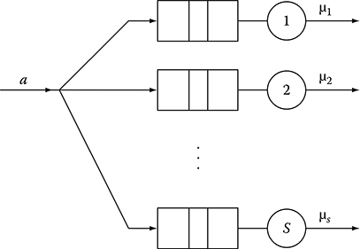
FIGURE 16.3 Queueing system with S parallel servers.

\min_{θ \in Θ} \sum_{i = 1}^{s} β_{i} J_{i} (n_{i}) s .t . \sum_{i = 1}^{s} n_{i} = K (16.16)

$\min_{θ \in Θ} \sum_{i = 1}^{s} β_{i} J_{i} (n_{i}) s .t . \sum_{i = 1}^{s} n_{i} = K (16.16)$

where 1 ≤ n_i ≤ K − S + 1 is the number of buffer units assigned to server i, J_i(n_i) is the blocking probability at queue i when allocated n_i buffer units, θ = [n₁, … , n_s] is an allocation vector and Θ is the set of all feasible allocation vectors. Finally, β_i is a weight associated with server i, but for simplicity, we will assume β_i = 1 for all i.

Typically, one is interested in solving Equation 16.16 when J_i(n_i) is of the form of an expectation J_i(n_i) = E [L_i(n_i, ω(n_i, [T₁, T₂]))] where L_i(n_i, ω(n_i, [T₁, T₂])) is a sample blocking probability observed at the system during the interval [T₁, T₂]. In general, there exists no closed-form solution for J_i(n_i) unless the system is driven by Poisson arrivals and exponential service times, all with known rates as well as known routing probabilities. Thus, a possible approach to solve this problem is to make an initial allocation θ₀ and observe the sample path of the system over the interval [0, T] (where T is a predefined period). Using the information extracted from the observed sample path, one can compute the sample performance metrics L_i(·), i = 1, … , S for the allocation θ₀ and use TWA to construct the sample paths for all other allocations θ ∈ Θ − {θ₀} and from them compute the corresponding sample performance functions. Consequently, at t = T, the controller can determine the allocation

θ*=arg min_{θ \in Θ} L (θ)

$θ*=arg min_{θ \in Θ} L (θ)$

where

L (θ) = \sum_{i = 1}^{s} L_{i} (n_{i}, ω (n_{i}, [0, T])), θ= [n_{1}, \dots, n_{s}] \in Θ

$L (θ) = \sum_{i = 1}^{s} L_{i} (n_{i}, ω (n_{i}, [0, T])), θ= [n_{1}, \dots, n_{s}] \in Θ$

Before proceeding any further, it is instructive to comment on an underlying assumption and two important parameters of the proposed optimization approach, namely, the length of the observation interval T and the cardinality of the set Θ. Note that the optimization approach uses data collected in the interval [0, T] to make buffer assignments that will be valid for t > T or, more precisely, for the interval [T, 2T]. Thus, the underlying assumption is that the future behavior of the system will be very similar to its past behavior. In other words, this approach is applicable to systems where the input stochastic processes that drive the system dynamics (in this example, the routing probabilities p_i(t), i = 1, … , S) change slowly compared to the observation interval T. Regarding the observation interval, its actual value depends on the variance of the input and output stochastic processes. If set too short, then the obtained performance metrics may be too noisy and, as a result, the controller may pick random allocations. On the contrary, T should not be set too large because the underlying assumption mentioned earlier may not be valid: if T is set too large and the behavior of the system has changed over time, then this will not be detected fast enough, and thus, the system may continue to operate at suboptimal allocations.

Regarding the cardinality of Θ, one can easily notice that it can become very large, which may cause computational problems due to the large number of sample paths that must be constructed. For the above example, the number of feasible allocations is $o (\frac{(K + S - 1)!}{K! (S - 1)!})$ $o (\frac{(K + S - 1)!}{K! (S - 1)!})$ . To alleviate the computational problem, one may resort to various optimization approaches taking advantage of some properties of the cost function. For the above example, we know that J_i(n_i) is decreasing and convex; thus, one may use “gradient”-based optimization approaches. In this case, we use finite differences together with a discrete resource allocation approach,¹⁶ which is briefly summarized below to reduce the number of constructed sample paths from $o (\frac{(K + S - 1)!}{K! (S - 1)!})$ $o (\frac{(K + S - 1)!}{K! (S - 1)!})$ to only S + 2. The idea of the discrete optimization approach is rather simple: at every step, it reallocates a resource (buffer) from the least “sensitive” server to the most sensitive one where sensitivity is defined as

Δ L_{i} (n_{i}) = L_{i} (n_{i}) - L_{i} (n_{i} - 1), n_{i} = 1, ..., K (16.17)

$Δ L_{i} (n_{i}) = L_{i} (n_{i}) - L_{i} (n_{i} - 1), n_{i} = 1, ..., K (16.17)$

Below are the detailed steps of the algorithm:

Algorithm: Dynamic Resource Allocation

1.0 Initialize: $θ_{0} = [n_{1}^{(0)}, ..., n_{S}^{(0)}]; C^{(0)} = {1, ..., S}; k = 0$ $θ_{0} = [n_{1}^{(0)}, ..., n_{S}^{(0)}]; C^{(0)} = {1, ..., S}; k = 0$

1.1 Evaluate $D^{(k)} (n_{1}^{(k)}, ...., n_{s}^{(k)}) \equiv [Δ L_{1} (n_{1}^{(k)}), ..., Δ L_{S} (n_{S}^{(k)})]$ $D^{(k)} (n_{1}^{(k)}, ...., n_{s}^{(k)}) \equiv [Δ L_{1} (n_{1}^{(k)}), ..., Δ L_{S} (n_{S}^{(k)})]$

2.1 Set $i^{*} = \arg \max_{i = 1, ..., C^{(k)}} [D^{(k)} (n_{1}^{(k)}, ..., n_{S}^{(k)})]$ $i^{*} = \arg \max_{i = 1, ..., C^{(k)}} [D^{(k)} (n_{1}^{(k)}, ..., n_{S}^{(k)})]$

2.2 Set $j^{*} = \arg \min_{i \in C (k)} [D^{(k)} (n_{1}^{(k)}, ..., n_{S}^{(k)})]$ $j^{*} = \arg \min_{i \in C (k)} [D^{(k)} (n_{1}^{(k)}, ..., n_{S}^{(k)})]$

2.3 Evaluate $D^{(k)} (n_{1}^{(k)}, \dots, n_{i}^{(k)} + 1, \dots, n_{j *}^{(k)} -, \dots, n_{s}^{(k)})$ $D^{(k)} (n_{1}^{(k)}, \dots, n_{i}^{(k)} + 1, \dots, n_{j *}^{(k)} -, \dots, n_{s}^{(k)})$

2.4 If $Δ L_{j *} (n_{j *}^{(k)} - 1) < Δ L_{i *} (n_{i *}^{(k)})$ $Δ L_{j *} (n_{j *}^{(k)} - 1) < Δ L_{i *} (n_{i *}^{(k)})$ Goto 3.1 ELSE Goto 3.2

3.1 Update allocation:

\begin{array}{l} n_{i *}^{(k + 1)} = n_{i *}^{(k)} + 1; n_{j *}^{(k + 1)} = n_{j *}^{(k)} - 1; n_{m}^{(k + 1)} = n_{m}^{k} for all m \in C^{(k)} and \\ m \neq i *, j *; \\ S e t k \leftarrow k + 1 \\ Reset C^{(k)} = {1, \dots, S}, and Goto 2 . 1 \end{array}

$\begin{array}{l} n_{i *}^{(k + 1)} = n_{i *}^{(k)} + 1; n_{j *}^{(k + 1)} = n_{j *}^{(k)} - 1; n_{m}^{(k + 1)} = n_{m}^{k} for all m \in C^{(k)} and \\ m \neq i *, j *; \\ S e t k \leftarrow k + 1 \\ Reset C^{(k)} = {1, \dots, S}, and Goto 2 . 1 \end{array}$

3.2 Replace C⁽^k⁾ by C⁽^k⁾ – {j^*};
IF |C⁽^k⁾| = 1, Reset C⁽^k⁾ = {1, … , S}, and Goto 2.1
ELSE Goto 2.2

When the system operates under a nominal allocation, one can obtain estimates of L_i(n_i) while concurrent estimators can provide estimates for L_i(n_i − 1); thus, the vector D^(k) (·) with all finite differences can be computed in step 1.1. Steps 2.1 and 2.2 determine the servers with the maximum and minimum finite differences i^* and j^*, respectively. Step 2.3 reevaluates the finite differences after a resource is reallocated from the least sensitive j^* to the most sensitive i^*. If the removal of the resource does not make j^* the most sensitive buffer, the reallocation is accepted in step 3.1, otherwise it is rejected in step 3.2.

Next, we consider a numerical example with S = 4 and K = 16. We assume that the arrival process is Poisson with rate λ = 1.3, and all service times (at any server) are exponential with rates µ_i = 1.0 for all i = 1, … , 4. At this point, we emphasize that the controller does not know anything about either the arrival or the service processes. Furthermore, we assume that the routing probabilities are also unknown to the controller and are time varying. Specifically, the routing probabilities change every 50,000 time units as given in Table 16.1.

Figure 16.4 presents the performance (loss probability) of the real-time controller (i.e., the dynamic resource allocation algorithm) in comparison to a static policy. Because of symmetry, the static optimal allocation is [4, 4, 4, 4], which achieves a loss probability between 0.08 and 0.1 for the entire simulation interval. As shown in the figure, the real-time controller can significantly improve the overall system performance since the real-time simulation components can “detect” the overloaded buffer and allocate more resources to it, thus reducing the overall loss probability. Initially, the controller adjusts the buffers such that the loss probability is between 0.02 and 0.04. At time 0.5 × 10⁵, the routing probabilities change abruptly, and thus, the loss probability significantly increases; however, as seen in the figure, the real-time controller quickly reallocates the buffers and the loss probability is again reduced. Similar behavior occurs every time the routing probabilities change.

In Figure 16.5, we also investigate the effect of the observation interval. The scenario investigated is identical to the one presented earlier. The only difference is the length of the observation interval T. In this experiment, we assume that the controller updates the allocation vector every NT observed events (here we use NT instead of T to indicate that the interval is determined by the number of events rather than time units). The figure presents the results for three different values of NT. As indicated in the figure, when NT is too large (NT = 7000), the controller does not capture the change in the routing probabilities, and as a result, it leaves the system operating at suboptimal allocations for long periods of time seriously degrading the overall system performance. On the contrary, when the observation interval is fairly short (NT = 166), the obtained estimates are fairly noisy, and as a result, the controller often makes “wrong” decisions, which also leads to poor performance.

TABLE 16.1
Routing Probabilities

From	To	Distribution
0	50,000	p₁ = [0.7, 0.1, 0.1, 0.1]
50,000	100,000	p₂ = [0.1, 0.7, 0.1, 0.1]
100,000	150,000	p₃ = [0.1, 0.1, 0.7, 0.1]
150,000	200,000	p₄ = [0.1, 0.1, 0.1, 0.7]

Images

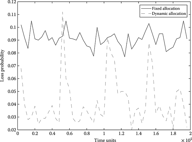
FIGURE 16.4 System performance under the dynamic allocation scheme versus a fixed resource allocation vector.

Images

FIGURE 16.5 System performance under different observation intervals.

16.6 Conclusions

This chapter has investigated the problem of real-time simulation for the online performance optimization of the policies or parameters of a DES. Given an observed sample path of a DES, the chapter has addressed the general sample path constructability problem and presented three concurrent simulation algorithms for solving the problem. The SC and the ASA approaches solve the problem very efficiently for a class of systems (although SC is more appropriate for offline simulation) with event lifetime distributions that satisfy the memoryless property. For more general systems, the TWA can be used to construct the sample paths of arbitrary DES using a sample path coupling approach. The TWA can be used in two modes, offline and online. In an offline setting, the objective of the TWA is to achieve a speedup factor greater than 1. On the contrary, in an online setting, the approach can be used for real-time control and optimization of DES. In this setting, the proposed concurrent simulation approach provides significant benefits since in general it does not require prior knowledge of the various event lifetime distributions. Furthermore, the approach inherently uses the CRN scheme that has been observed experimentally and was proved theoretically in some cases to be effective in variance reduction.¹⁷

Acknowledgments

The work of Christos Cassandras was supported in part by NSF under Grant EFRI-0735974, by AFOSR under grants FA9550-07-1-0361 and FA9550-09-1-0095, by DOE under grant DE-FG52-06NA27490, and by ONR under grant N00014-09-1-1051.

The work of Christos G. Panayiotou was supported in part by the Cyprus Research Promotion Foundation, the European Regional Development Fund, the Government of Cyprus, and by the European Project Control for Coordination of distributed systems (CON4COORD - FP7-2007-IST-2-223844).

References

1. Fujimoto, M. R. 2000. Parallel and Distributed Simulation Systems. New York: Wiley Interscience.

2. Boer, C. A., A. de Bruin, and A. Verbraeck. 2008. “Distributed Simulation In Industry—A Survey, Part 3—The HLA Standard in Industry.” In Proceedings of the 40th Conference on Winter Simulation, WSC ’08, 1094–102.

3. Cassandras, C. G., and S. Lafortune. 2007. Introduction to Discrete Event Systems. New York: Springer.

4. Cassandras, C. G., and C. G. Panayiotou. 1999. “Concurrent Sample Path Analysis of Discrete Event Systems.” Journal of Discrete Event Dynamic Systems: Theory and Applications 9 (2): 171–95.

5. Cassandras, C. G., and V. Julka. 1994. “Descent Algorithms for Discrete Resource Allocation Problems.” In Proceedings of the IEEE 33rd Conference on Decision and Control, 2639–44.

6. Panayiotou, C. G., and C. G. Cassandras. 1999. “Optimization of Kanban-Based Manufacturing Systems.” Automatica 35 (9): 1521–33.

7. Yan, D., and H. Mukai. 1992. “Stochastic Discrete Optimization.” SIAM Journal on Control and Optimization, 30 (3): 594–612.

8. Gong, W.-B., Y. C. Ho, and W. Zhai. 1992. “Stochastic Comparison Algorithm for Discrete Optimization with Estimation.” In Proceedings of 31st IEEE Conference on Decision and Control, 795–802.

9. Panayiotou, C. G., and C. G. Cassandras. 2001. “On-Line Predictive Techniques for ‘Differentiated Services’ Networks.” In Proceedings of IEEE Conference on Decision and Control, 4529–34.

10. Panayiotou, C. G., and C. G. Cassandras. 1997. “Dynamic Resource Allocation in Discrete Event Systems.” In Proceedings of IEEE Mediterranean Conference on Control and Systems.

11. Vakili, P. 1991. “Using a Standard Clock Technique for Efficient Simulation.” Operations Research Letters 10 (8): 445–52.

12. Cassandras, C. G., and S. G. Strickland. 1989. “On-Line Sensitivity Analysis of Markov Chains.” IEEE Transactions on Automatic Control 34 (1): 76–86.

13. Cassandras, C. G., and S. G. Strickland. 1989. “Observable Augmented Systems for Sensitivity Analysis of Markov and Semi-Markov Processes.” IEEE Transactions on Automatic Control 34 (10): 1026–37.

14. Park, Y., and E. K. P. Chong. 1995. “Distributed Inversion in Timed Discrete Event Systems.” Journal of Discrete Event Dynamic Systems 5(2/3), 219–41.

15. Cassandras, C. G., and W. Shi. 1996. “Perturbation Analysis of Multiclass Multiobjective Queueing Systems with ‘Quality-of-Service’ Guarantees.” In Proceedings of the IEEE 35th Conference on Decision and Control, 3322–7.

16. Cassandras, C. G., L. Dai, and C.G. Panayiotou. 1998. “Ordinal Optimization for a Class of Deterministic and Stochastic Discrete Resource Allocation Problems.” IEEE Transactions on Automatic Control 43 (7), 881–900.

17. Dai, L., and C. H. Chen. 1997. “Rates of Convergence of Ordinal Comparison for Dependent Discrete Event Dynamic Systems.” Journal of Optimization Theory and Applications 94 (1): 29–54.

..................Content has been hidden....................

You can't read the all page of ebook, please click here login for view all page.

Table of Contents for
Chapter 16 Concurrent Simulation for Online Optimization of Discrete Event Systems

16 Concurrent Simulation for Online Optimization of Discrete Event Systems

CONTENTS

16.1 Introduction

16.2 Modeling and Simulating Discrete Event Systems

16.3 Sample Path Constructability

16.3.1 Standard Clock Approach

16.3.2 Augmented System Analysis