
23 Real-Time Simulation of Physical Systems Using Simscape™
Steve Miller and Jeff Wendlandt
CONTENTS
23.1.1 Examples of Real-Time Simulation
23.1.2 Benefits of Real-Time Simulation
23.1.3 Challenges of Real-Time Simulation
23.2 Moving from Desktop to Real-Time Simulation
23.2.1 Procedure for Tuning Solver Settings
23.1 Introduction
Real-time simulation of multidomain physical system models (mechanical, electrical, hydraulic, etc.) requires finding a combination of model complexity, solver choice, solver settings, and real-time target that permit execution in real time. A better understanding of the trade-offs involved in each of these areas makes it easier to achieve this goal and use Model-Based Design to reap the benefits of using virtual systems before building hardware prototypes. This chapter outlines the steps in moving from desktop to real-time simulation and illustrates this process using models built from MathWorks® products based on Simscape™ simulation technology. The steps described apply to real-time simulation regardless of which real-time hardware is used.
23.1.1 Examples of Real-Time Simulation
Replacing physical devices, such as vehicles, robots, or planes, with virtual devices can drastically reduce the cost of testing control systems, software, and hardware. It can also improve the quality of the final product by enabling more complete testing of the entire system. Often it is necessary to run the computer simulation representing the virtual system in real time. This means that the inputs and outputs (I/O) in the virtual world of simulation must be read or updated synchronously with the physical world. When the simulation time reaches 5, 50, or 500 seconds, the exact same amount of time has passed in the physical world.
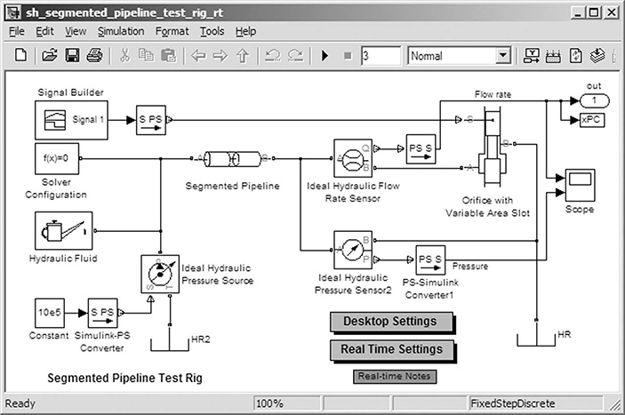
FIGURE 23.1 SimHydraulics demonstration model of water hammer in a pipeline.
Configuring a model and the numerical integrator to simulate in this manner can be difficult. The simulation execution time per step must be consistent and sufficiently shorter than the time step of the simulation to permit any other tasks that the simulation environment must perform, such as reading sensor inputs or outputting transducer signals. This is a challenging prospect because the conditions vary during simulation. Switches open, valves close, and these occasional events can require more computations to achieve an accurate result. To be successful, the solver settings, simulation step size, and the level of model fidelity must be adjusted to find a combination that permits real-time simulation while delivering accurate results.
Advances in solver technology have made it easier to configure simulations to simulate in this fashion. Features added to simulation tools, such as fixed-cost algorithms (algorithms where the computational cost per time step is nearly constant) and local solvers added to Simscape from MathWorks, make it possible to simulate even complex models such as hydraulic pipelines in real time. As an example, we simulated the SimHydraulics® demonstration model sh_segmented_pipeline_test_ rig (Figure 23.1) on a desktop computer using solver ode15s, a maximum step size of 0.03 seconds, and a relative tolerance of 1e-3. After applying the process covered in this chapter to the model, accurate results were achieved when running the model in real time using xPC Target™ [1] from MathWorks on an Intel Core 2 Duo E6700 (2.66 GHz) with a simulation step size of 1 millisecond (Figure 23.2).
This is a particularly challenging model numerically for it includes the water hammer effect, which takes place when a valve is abruptly opened or closed creating rapid changes in flow rate. Even with the restrictions imposed by executing on a real-time target, the simulation results capture the oscillations in the hydraulic circuit. To develop this process, the steps described in this chapter for moving from desktop to real-time simulation have been applied to this and more than 30 other models in different physical domains built with MathWorks physical modeling products, all of which were able to run in real time.
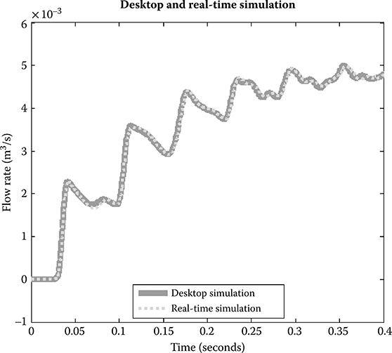
FIGURE 23.2 Desktop and real-time simulation results. The results are nearly identical.
23.1.2 Benefits of Real-Time Simulation
Real-time simulation is used in a number of steps in the development process and in some cases in the final product. In Model-Based Design, the plant model is used to develop and test the control and signal processing algorithms in desktop simulation. Once the designs are complete and the algorithms exist in production code, it is necessary to test that code as well as the production controller. Instead of connecting it directly to a hardware prototype, the plant model used in the design phase can be used to test the production code and processor if it is capable of running in real time. This is referred to as hardware-in-the-loop testing and offers many benefits, including the following:
Ability to test conditions that would damage equipment or personnel
Ability to test systems where no prototypes exist
Reduced costs in the later phases of development
Ability to test 24 hours a day, 7 days a week
In addition to the development process, real-time simulation is also used in the final product. Products that have a human in the simulation loop require real-time simulation. For example, flight simulators that are used to train pilots require real-time simulation of the plane, control system, weather conditions, and other aspects of their environment (see also Chapter 15).
23.1.3 Challenges of Real-Time Simulation
For a simulation to execute in real time, the amount of time spent calculating the solution for a given time step must be less than the duration of that time step. This requires that the execution time per simulation time step be bounded. Variable-step solvers, which are often used in desktop simulation, take smaller steps to accurately capture events that occur during the simulation. However, varying the step size is not an option for real-time simulation, and therefore, a fixed-step solver (implicit or explicit) must be used. This can make real-time simulation more challenging than desktop simulation. The model and fixed-step solvers must be configured so that system dynamics can be accurately captured without changing the step size. These requirements are constraints imposed by hard real-time systems, such as those used to test controller software and hardware. Soft real-time systems, such as video game physics, often have less stringent requirements.
A fixed-step solver that provides accurate results at a step size large enough to permit real-time simulation must be chosen. Most fixed-step solvers will produce equally accurate simulation results as a variable-step solver if a small enough step size is chosen. However, different fixed-step solver algorithms (implicit, explicit, lower/higher order, etc.) will require different step sizes to produce accurate results. They also require different amounts of computational effort per time step [2].
Once a solver is chosen, determining an appropriate step size is the next challenge. Increasing the time step to permit more time to calculate the result can lead to inaccurate results. Reducing the time step to improve the accuracy of the simulation results may make it impossible to execute in real time. Trial and error may be required to find the combination of settings that permit real-time simulation while producing accurate simulation results. The eigenvalues [3] of the system can give an indication of the time constants in the system and help determine what the required minimum step size is.
If this combination of settings cannot be found, it may be that the model contains effects that a fixed-step solver cannot handle at a step size that permits real-time simulation. These effects can be events in the simulation (hard stops, stick-slip friction, switches that open and close, etc.) or portions of the system that have a very small time constant (small masses attached to stiff springs, current or pressure oscillations, etc.). Identifying and modifying these elements is then required before searching for the combination of solver settings and step size that will permit real-time simulation.
Section 23.2 will cover the process of configuring a model used in desktop simulation for real-time simulation. The process involves determining if the model is built at an appropriate level of fidelity for real-time simulation, simplifying if necessary, and configuring solver settings to achieve accurate results.
23.2 Moving from Desktop to Real-Time Simulation
To move from desktop simulation to real-time simulation on the chosen real-time hardware, the following items must be adjusted until the simulation can execute in real time and deliver results sufficiently close to the results obtained from desktop simulation:
Solver choice
Number of solver iterations
Step size
Model size and fidelity
The procedure depicted in the flowchart in Figure 23.3 shows how to configure a model for real-time simulation.
This process has been applied to over 30 models containing hydraulic, electrical, mechanical, pneumatic, and thermal components that include a range of linear and nonlinear elements. In each case, real-time execution was achieved with very accurate results. The modeling concepts in these models included the following:
Combined multibody (3D-mechanical) and hydraulic or electrical systems
Dynamic, compressible fluid flow (hydraulic and pneumatic)
Physical phenomena (friction and clutch events)
Hybrid models (continuous-time plants plus discrete logic control systems)
Multirate systems (multiple sample rates within the model)
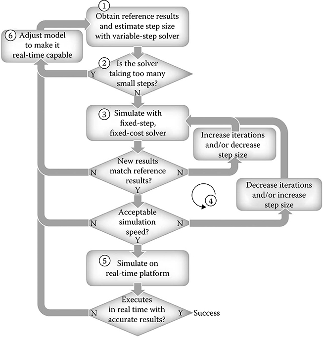
FIGURE 23.3 Flowchart depicting the process that helps engineers move from desktop simulation to real-time simulation.
23.2.1 Procedure for Tuning Solver Settings
Step 1: Obtain a converged set of results with a variable-step solver.
To ensure that the results obtained with the fixed-step solver are accurate, a set of reference results are needed. These can be obtained by simulating the system with a variable-step solver and ensuring that the results are converged by tightening the error tolerances until the simulation results do not change. For Simscape models, the recommended variable-step solvers are ode15s and ode23t.
Step 2: Examine the step sizes during the simulation to determine if the model is likely to run with a large enough step size to permit real-time simulation.
A variable-step solver will vary the step size to stay within the error tolerances and to react to zero-crossing events [4]. If the solver abruptly reduces the step size to a small value (e.g., 1e-15s), this indicates that the solver is attempting to accurately identify a zero-crossing event. A fixed-step solver may have trouble capturing these events at a step size that is sufficiently large to permit real-time simulation.
The following MATLAB® commands can be used to generate a plot that shows how the time step varies during the simulation:
semilogy(tout(1:end-1),diff(tout),‘-*’); title(‘Step Size vs. Simulation Time’,‘FontSize’,14,‘FontWeight’,‘bold’); xlabel(‘Simulation Time (s)’,‘FontSize’,12); ylabel(‘Step Size (s)’,‘FontSize’,12);The plots in Figures 23.4 and 23.5 illustrate the concepts explained above. They are produced by executing the preceding MATLAB code on the simulation results from the SimHydraulics model shown in Figures 23.6 and 23.7, which contains a number of components that create zero-crossing events.
This analysis should provide a rough idea of a step size that can be used to run the simulation. Determining what effects are causing these events and modifying or eliminating them will make it easier to run the system with a fixed-step solver at a larger step size and produce results comparable to the variable-step simulation.
Step 3: Simulate the system with a fixed-step, fixed-cost solver and compare the results to the reference set of results obtained from the variable-step simulation.
As explained in Section 23.1.3, a fixed-step solver (implicit or explicit) must be used to run the simulation in real time. The chosen solver must provide robust performance and deliver accurate results at a step size large enough to permit real-time simulation. The solver should be chosen to minimize the amount of computation required per time step while providing robust performance at the largest step size possible. To decide which type of fixed-step solver to use, it is necessary to determine if the model describes a stiff or a nonstiff problem. The problem is stiff if the solution the solver is seeking varies slowly, but there are other solutions within the error tolerances that vary rapidly [2].
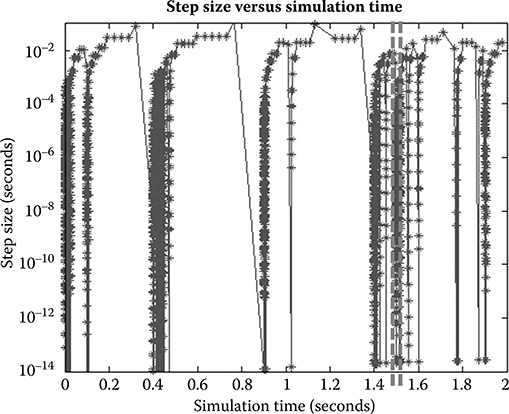
FIGURE 23.4 Plot of step size during variable-step simulation. Abrupt drops in step size indicate zero-crossing events. The amount of zero-crossing events and how easily the simulation recovers give a rough indication of how difficult it will be for a fixed-step solver to produce accurate results at the largest step size the variable-step solver uses.
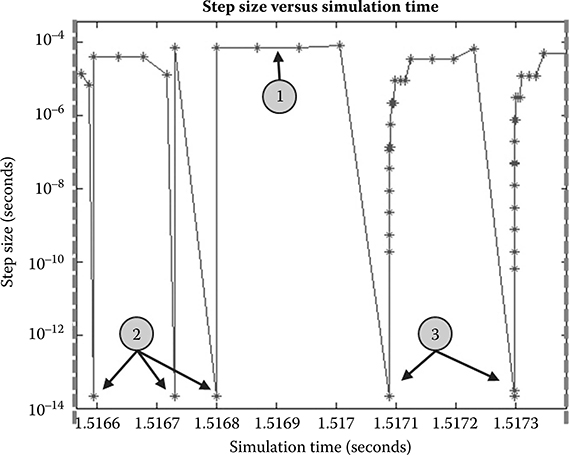
FIGURE 23.5 Plot of a smaller range of the step size during simulation. (1) indicates the step size that will meet the error tolerances for most of the simulation. (2) are examples of zero-crossing events where the solver recovered instantly and may not be difficult for the fixed-step solver. (3) are examples of zero-crossing events where the variable-step solver took longer to recover and will likely require a smaller step size for the fixed-step solver to deliver results with acceptable accuracy.
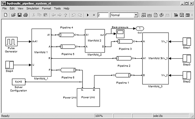
FIGURE 23.6 Hydraulic model of a pipeline system modeled in SimHydraulics containing valves, junctions, and a centrifugal pump.
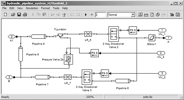
FIGURE 23.7 Portion of SimHydraulics model containing directional valves, flow control valves, and orifices.
Comparing the simulation results generated by a fixed-step implicit solver and a fixed-step explicit solver for the same model of a pneumatic system (Figure 23.8) shows a difference in accuracy that is dependent on step size (Figure 23.9) and model stiffness (Figure 23.10).
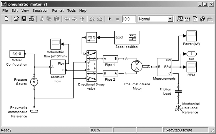
FIGURE 23.8 Pneumatic system containing a pump, valve, and motor, simulated using implicit and explicit fixed-step solvers.
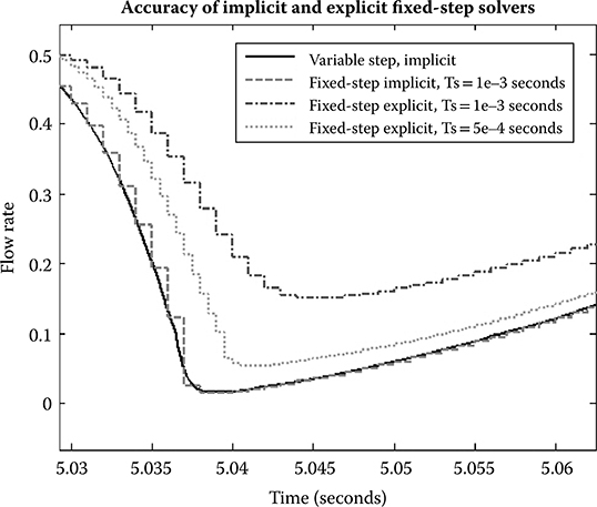
FIGURE 23.9 Plot showing simulation results for the same model simulated with a variable-step solver, fixed-step implicit solver, and fixed-step explicit solver. The explicit solver requires a smaller time step to achieve accuracy comparable to the implicit solver.
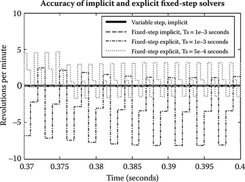
FIGURE 23.10 Plot showing simulation results for the same model simulated with a variable-step solver, fixed-step implicit solver, and fixed-step explicit solver. The oscillations in the fixed-step explicit solver simulation results suggest this is a stiff problem.
Explicit and implicit solvers use different numerical methods to solve the system of equations. An explicit algorithm samples the local gradient to find a solution, whereas an implicit algorithm uses matrix operations to solve a system of simultaneous equations that helps predict the evolution of the solution [2]. As a result, an implicit algorithm does more work per simulation step but can take larger steps. For stiff systems, implicit solvers should be used.
Both accuracy and computational effort must be taken into account when choosing a fixed-step solver. Simulating physical systems often involves multiple iterations per time step to converge on a solution. For a real-time simulation, the amount of computational effort per time step must be bounded. To have a bounded amount of execution time per simulation time step, it is necessary to limit the number of iterations per time step. This is known as a fixed-cost simulation. Fixed-cost simulation is used to prevent overruns, which occur when the execution time is longer than the sample time. Figure 23.11 shows how an overrun can occur if the number of iterations is not limited.
Iterations are necessary with implicit solvers. The iterations are handled automatically with variable-step solvers, but for the implicit fixed-step solver ode14x in Simulink®, the number of iterations per time step must be set. This is controlled by the parameter “Number Newton’s iterations” in the Solver pane of the Configuration Parameters dialog box in Simulink.
Iterations are also often necessary for each Simscape physical network for both explicit and implicit solvers. The iterations in Simscape are limited by setting the checkbox, “Use fixed-cost runtime consistency iterations” and entering the number of nonlinear iterations in the Solver Configuration block (see Figure 23.12). If the local solver option is used, it is recommended to initially set the number of nonlinear iterations to two or three.
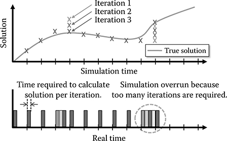
FIGURE 23.11 A fixed-step solver keeps the time step constant. Limiting any needed iterations per time step is necessary for fixed-cost simulation.
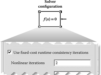
FIGURE 23.12 In Simscape, the Solver Configuration block permits limitation of the iterations per time step.
The amount of computational effort required by a solver varies with respect to a number of factors, including model complexity. To provide an indication of the relative cost for the fixed-step solvers available, a nonlinear model of a pneumatic actuation system (shown in Figure 23.8) containing a single Simscape physical network was simulated with each of the fixed-step solvers. These simulations were conducted at the same step size with similar settings for the total number of solver iterations. Figure 23.13 shows the normalized execution time.
From this plot, it is clear that for this example, most explicit fixed-step solvers require less computational effort than the implicit fixed-step solver ode14x. Although an explicit solver may require less computational effort, for stiff problems, an implicit solver is necessary for accurate results. For this example, the two local Simscape solvers (Backward Euler and Trapezoidal Rule) required the least computational effort. In most cases, they provide the best combination of speed and accuracy.
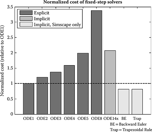
FIGURE 23.13 Plot of the normalized cost of all fixed-step solvers that can be used on Simscape models. The results were obtained by simulating a nonlinear model containing a single Simscape physical network with each solver at the same step size and similar settings for the total number of solver iterations.
A powerful option available in Simscape is to use a local solver on physical networks [5] . By using this option, it is possible to use an implicit fixed-step solver only on the stiff portions of the model and an explicit fixed-step solver on the remainder of the model (Figure 23.14). This minimizes the computations performed per time step, making it more likely the model will run in real time.
For Simscape models, the Backward Euler and the Trapezoidal Rule should always be tested and will most likely provide the best performance and the most flexibility because they can be configured per physical network. Figure 23.15 shows how to enable the local solver and the settings associated with it. The Backward Euler solver is designed to be robust and tends to damp out oscillations. The Trapezoidal Rule solver is designed to be more accurate and preserve oscillations. The Backward Euler algorithm tends to be less accurate than the Trapezoidal Rule but more numerically stable.
To summarize recommendations for setting up fixed-cost simulations:
If the system is nonstiff and is described by ordinary differential equations (ODEs), an explicit solver is usually the best choice.
If the system is stiff, an implicit solver (ode14x, Backward Euler, or Trapezoidal Rule) should be used and the number of iterations must be limited.
For Simscape models:
Performing a fixed-cost simulation requires setting the number of iterations to prevent overruns. This is done by selecting the “Use fixed-cost runtime consistency iterations” setting in the Solver Configuration block attached to the Simscape physical network.
The local solvers in Simscape should always be tested. Using a local solver is often the best choice for fixed-cost simulations.
When performing fixed-cost simulation using the local solvers in Simscape, it is recommended to initially set the number of nonlinear iterations to two or three.
If you are using ode14x on a model with a Simscape physical network, to perform a fixed-cost simulation, it is necessary to enable fixed cost and set the number of nonlinear iterations in the Solver Configuration block.
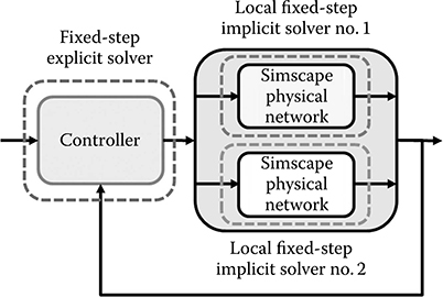
FIGURE 23.14 Using local solvers permits configuring implicit solvers on the stiff portions of the model and explicit solvers on the remainder of the model, minimizing execution time while maintaining accuracy.
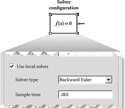
FIGURE 23.15 In Simscape, the Solver Configuration block permits configuration of local solvers on Simscape physical networks.
Step 4: Find the combination of step size and number of nonlinear iterations where the step size is small enough to produce results that are sufficiently close to the set of reference results obtained from variable-step simulation and large enough so that there is enough safety margin to prevent an overrun.
During each time step, the real-time system must calculate the simulation results for the next time step (simulation execution) and read the inputs and write the outputs (processing I/O and other tasks). If this takes less than the specified time step, the processor remains idle during the remainder of the step. These quantities are illustrated in Figure 23.16.
The challenge is to find appropriate settings that provide accurate results while permitting real-time simulation. In each case, it is a trade-off of accuracy versus speed. Choosing a computationally intensive solver, increasing the number of nonlinear iterations, or reducing the step size both increases the accuracy and reduces the amount of idle time, raising the risk that the simulation will not run in real time. Adjusting these settings in the opposite direction will increase the amount of idle time but reduce accuracy.
It is necessary to leave sufficient safety margin to avoid an overrun when simulating in real time. If the amount of time spent processing inputs, outputs, and other tasks as well as the desired percentage of idle time are known, the amount of time available for simulation execution can be calculated as follows:
Estimating the budget for the execution time helps ensure a feasible combination of settings is chosen.
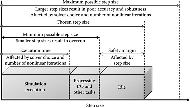
FIGURE 23.16 Trade-off involving solver choice, number of nonlinear iterations, and step size. For a given model, these must be chosen to deliver maximum accuracy and robustness with enough idle time to provide a sufficient safety margin.
The speed of simulation on the desktop can be used to estimate the execution time on the real-time target. There are many factors that affect the execution time on the real-time target, and therefore, simply comparing processor speed may not be sufficient. A better method is to measure the execution time during desktop simulation and then to determine the average execution time per time step on the real-time target for a given model. Knowing how these values relate for one model makes it possible to estimate execution time on the real-time target from the execution time during desktop simulation when testing other models.
Step 5: Using the selected solver, number of nonlinear iterations, and step size, simulate on the real-time platform and determine if the simulation can run in real time. The tests run on the real-time platform should cover a representative set of tests to ensure that the worst-case scenario for the idle time is captured. This may include varying parameter values, inputs, and a range of conditions for the external hardware (reading/writing the I/O). The model needs to be robust enough to handle all situations that it may encounter.
Step 6: If the simulation does not run in real time on the selected real-time platform, it will be necessary to determine the cause and choose an appropriate solution.
If the simulation does not run in real time on the real-time platform, it may be due to the fact that the model is not real-time capable. The combination of effects captured in the model and the speed of the real-time platform may make it impossible to find solver settings that will permit it to run in real time (Figure 23.17).
If the simulation is not real-time capable, there are some options that can be explored:
Use a faster real-time computer.
Determine new settings that reduce the execution time (e.g., reducing the number of nonlinear iterations) or permit a larger step size.
Eliminate effects that require significant computational effort or that require a small time step to accurately capture them.
If possible, configure the model and the real-time system to evaluate the physical networks in parallel. This can be done if for a given time step the networks are not dependent on one another. Experience with the generated code and the real-time target is required to use this option.
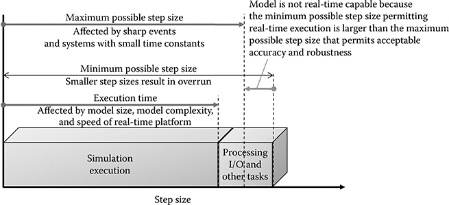
FIGURE 23.17 Diagram showing when a simulation is not real-time capable. The minimum possible step size permitting real-time execution is larger than the maximum possible step size that permits acceptable accuracy and robustness.
23.2.2 Adjusting Models to Make Them Real-Time Capable
In the event that no settings can be found that permit the simulation to run in real time on the available real-time computer while delivering accurate results, it is necessary to modify or remove effects from the model that prevent real-time simulation. Here are two categories and some examples.
Elements that create events
In this case, an event occurs so that the solution changes nearly instantaneously. The rapid change can be difficult for a fixed-step solver to step over and find the correct solution on the other side of the event. If it fails to find the solution, the solver may go unstable. Examples of elements that create these kinds of events include the following:
Hard stops, backlash
Stick-slip friction
Switches or clutches
Elements with a small time constant
In this case, an element or a group of elements has a very small time constant as compared to the desired simulation step size. These elements create fast dynamics that require a small step size so that a fixed-step solver can accurately capture the dynamics. Examples of systems that have a small time constant include the following:
Small masses attached to stiff springs with minimal damping
Electrical circuits with fast dynamics
Hydraulic circuits with small compressible volumes
If a scripting environment that has commands permitting interrogation of the model, such as MATLAB, is available, identifying these components and parameters can be done very quickly, which narrows the search for the effects that must be modified. There are methods to automate these searches using tools such as the Simulink Model Advisor that makes it easier to apply these searches to other models.
Examining the eigenmodes of the system can indicate which states have the highest frequency, and mapping those states to the individual components may point to the source of the problem. For nonlinear models, this can only be done at an individual operating point and that operating point can be identified by looking for small step sizes during a variable-step simulation.
Once the effects have been identified, the next step is to modify or eliminate them. Methods that can be used to modify these effects include the following:
Replacing nonlinear component models with linearized versions of those models
Using lookup tables to simplify complex equations
Producing a simplified model by using system identification theory on the I/O data
Smoothing discontinuous functions (step changes) by using filters and other techniques.
Once the model is modified, the process described in Section 23.2 can be applied to identify the appropriate solver configuration and settings to enable real-time simulation.
23.3 Results and Conclusions
The procedure described in this chapter has been applied to over 30 physical models built using Simscape, SimHydraulics, and SimElectronics®, and all of them are able to run in real time. These models contain hydraulic, electrical, mechanical, pneumatic, and thermal elements and include applications such as hydromechanical servovalves, brushless DC motors, hydraulic pipelines with water hammer effects, and pneumatic actuation systems with stick-slip friction. Nearly all of the models are nonlinear. As an indication of the size of the models, after equation reduction, the smallest model had 4 states and the largest model had 117 states. The original number of states before equation reduction is typically much larger.
All simulations were performed on an Intel Core 2 Duo E6700 (2.66 GHz) that was running xPC Target from MathWorks. With each model, settings that permitted real-time simulation on the target and delivered accurate results with more than enough idle time to ensure robust simulation were found. The maximum percentage of a step spent in simulation execution was less than 18%, meaning that there was plenty of safety margin for processing I/O and other tasks. The average percentage spent in simulation execution was 3.9% and the minimum was 6e-4%.
This chapter covered the background of real-time simulation and described the steps in moving from desktop to real-time simulation. Balancing the trade-off of model fidelity and simulation speed is a core challenge of moving from desktop to real-time simulation. Simscape local solvers permit a lot of flexibility for adjusting the amount of computation done per time step by permitting different sample rates and setting the number of iterations per time step. The benefits of real-time simulation are significant, including reduced development costs and higher quality products. As a core element of Model-Based Design, it will continue to play an important role in product development processes.
References
1. MathWorks. 2012. xPC User’s Guide. Natick, MA: MathWorks.
2. Moler, C. 2003. Stiff Differential Equations. MATLAB News and Notes. http://www.mathworks.com/company/newsletters/news_notes/clevescorner/may03_cleve.html.
3. Strang, G. 1988. Linear Algebra and Its Applications, February. San Diego, CA: Harcourth Brace Jovanovich.
4. MathWorks. 2012. Simulink User’s Guide. Natick, MA: MathWorks. http://www.mathworks.com/access/helpdesk/help/toolbox/simulink/ug/f7-8243.html#f7-9506.
5. MathWorks. 2012. Simscape User’s Guide. Natick, MA: MathWorks.