Because join is so important, and because there are so many issues we need to discuss in connection with it, I’ve decided to split my treatment of the topic into three separate chapters. In this first one, I want to limit my attention to what might be regarded as the simplest possible case: viz., the case in which the join in question is a one to one join specifically. As usual, I’ll base my discussions on some simple examples.

My first example is effectively the inverse of the first of the projection examples from the previous chapter. (As noted in that chapter, there’s a tight connection between join views and projection views in general.) To be specific, suppose we’re given base relvars ST and SC, looking like this (in outline):

ST { SNO , STATUS } KEY { SNO }
SC { SNO , CITY } KEY { SNO }

(As in Chapter 5, I ignore attribute SNAME for simplicity.) Now suppose we define the join of these two relvars, ST JOIN SC, as a view S:

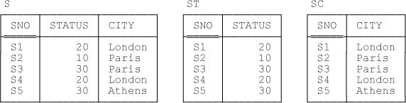
S { SNO , STATUS , CITY } KEY { SNO }

Further, let’s assume this join is strictly one to one, in the sense that every tuple in ST joins to exactly one tuple in SC and vice versa. In other words, we have information equivalence—the design consisting of ST and SC taken together and the design consisting of just view S are clearly information equivalent. Sample values are shown in Figure 6-1 (of course, that figure is identical to Figure 5-1 in Chapter 5, but now ST and SC are base relvars and S is a view).

Figure 6-1. Relvars S, ST, and SC—sample values

Here’s the predicate for the join (of course, it’s basically the usual predicate for relvar S, but simplified to take account of the fact that we’ve dropped attribute SNAME):

As usual, the first thing to do is consider what happens if all three relvars are base ones. But we’ve already done that, in the discussion of Example 1 in Chapter 5! So let me just repeat here the salient points from that discussion. First, as already indicated, each of the three relvars has {SNO} as its sole key. The following constraints also hold (as noted in Chapter 5, they’re all equality dependencies (EQDs), and together they ensure that the two designs are, as I’ve already said, information equivalent):

CONSTRAINT ... S  = JOIN { ST , SC } ;
CONSTRAINT ... ST = S { SNO , STATUS } ;
CONSTRAINT ... SC = S { SNO , CITY } ;
CONSTRAINT ... IDENTICAL { S { SNO } , ST { SNO } , SC { SNO } } ;

Actually, if you check, you’ll see I gave these constraints in a different order in the previous chapter. I’ve reordered them here to show that, first, S is indeed equal to the join of the other two relvars; next—in order to guarantee the desired information equivalence—ST and SC are indeed equal to the corresponding projections of S; and finally, every supplier number appearing in S also appears in both ST and SC and vice versa. Note: In fact, of course, this final constraint is a logical consequence of certain of the other three constraints taken together (which ones, exactly?).

The compensatory actions are the same as before, too, though again I’ve changed the sequence:

ON DELETE dt FROM ST , DELETE dc FROM SC ,
   INSERT it INTO ST , INSERT ic INTO SC :
   WITH ( t1 := it JOIN SC , t2 := ic JOIN ST ,
          t3 := S MATCHING dt , t4 := S MATCHING dc ) :
   INSERT t1 INTO S ,
   INSERT t2 INTO S ,
   DELETE t3 FROM S ,
   DELETE t4 FROM S ;

ON DELETE d FROM S , INSERT i INTO S :
   DELETE d { SNO , STATUS } FROM ST ,
   DELETE d { SNO , CITY } FROM SC ,
   INSERT i { SNO , STATUS } INTO ST ,
   INSERT i { SNO , CITY } INTO SC ;

Let me remind you also that INSERT and “key UPDATE” operations on ST and SC must be “double updates,” for otherwise they’ll fail on a Golden Rule violation.

Now suppose as we originally did that S is in fact a view, the join of ST and SC. Then:

Also, a user who sees only the join view S can behave in all respects exactly as if that view were a base relvar. Such a user will be aware of the fact that {SNO} is a key (but not of any other constraints, nor of any compensatory actions), and will be aware also of the corresponding predicate:

And, to spell the point out, INSERTs, DELETEs, and explicit UPDATEs on that view S all work exactly as they would if S were a base relvar instead.

So updating a one to one join view, in the case where we have information equivalence, is essentially straightforward. But what if we’re dealing with an information hiding situation? By way of a concrete example, suppose a supplier can be represented in base relvar ST and not base relvar SC or the other way around; in other words, instead of requiring every supplier to have both a status and a city, as we did in Example 1, suppose now only that every supplier is required to have at least one of those two properties.^[82] Then the join S of ST and SC loses information, inasmuch as it’s no longer guaranteed that ST and SC are equal to the projections of that join on the appropriate attributes. In fact, of the constraints mentioned in the previous section, the only ones that continue to hold are the usual key constraints ({SNO} is a key for each of S, ST, and SC), together with this one:^[83]

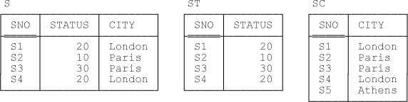
CONSTRAINT ... S = JOIN { ST , SC } ;

Sample values satisfying the foregoing conditions can be obtained by modifying Figure 6-1 to remove the tuple for supplier S5 from each of relvars S and ST but not from relvar SC (see Figure 6-2). Of course, the predicate for S is still as it was for Example 1.

Figure 6-2. A revised version of Figure 6-1

Back to Example 2. Let me now stress the fact that, precisely because the join view S loses information, a database containing just that view isn’t information equivalent to one containing base relvars ST and SC. (An example of a query on the latter that has no counterpart on the former is “Get supplier numbers for suppliers who have a city but no status.”) More precisely, any information that can be represented by S alone can certainly be represented by the combination of ST and SC, but the converse is false. As a consequence, it’s obvious that there’ll be updates on ST and/or SC that have no counterpart on S. An example is “Insert a tuple into SC for a supplier with supplier number S9 and city London,” without simultaneously inserting a tuple for that same supplier S9 into ST.

So what compensatory actions apply? Well, since there’s no longer a strict one to one relationship between relvars ST and SC, it’s now possible as just indicated to insert into, or delete from, just one of the two without simultaneously inserting into or deleting from the other. Thus, since S is required to be at all times equal to the join of ST and SC, we clearly have:

ON INSERT it INTO ST , INSERT ic INTO SC :
   INSERT ( it JOIN SC ) INTO S ,
   INSERT ( ic JOIN ST ) INTO S ;

ON DELETE dt FROM ST , DELETE dc FROM SC :
   DELETE ( S MATCHING dt ) FROM S ,
   DELETE ( S MATCHING dc ) FROM S ;

Now, I’ve shown these rules separately for reasons of clarity, but of course they can be combined into one:

ON DELETE dt FROM ST , DELETE dc FROM SC ,
   INSERT it INTO ST , INSERT ic INTO SC :
   DELETE ( S MATCHING dt ) FROM S ,
   DELETE ( S MATCHING dc ) FROM S ,
   INSERT ( it JOIN SC ) INTO S ,
   INSERT ( ic JOIN ST ) INTO S ;

And if you compare this rule with the corresponding rule for Example 1 from the previous section—the strict one to one case—you’ll see it’s essentially identical (except that I used some introduced names in that previous section, for clarity). Here in order to make it easier to do the comparison is that previous rule:

ON DELETE dt FROM ST , DELETE dc FROM SC ,
   INSERT it INTO ST , INSERT ic INTO SC :
   WITH ( t1 := it JOIN SC , t2 := ic JOIN ST ,
          t3 := S MATCHING dt , t4 := S MATCHING dc ) :
   INSERT t1 INTO S ,
   INSERT t2 INTO S ,
   DELETE t3 FROM S ,
   DELETE t4 FROM S ;

So much for updates on ST and/or SC. But what about the join view?—i.e., what happens if we do INSERTs or DELETEs on S, instead of on ST and/or SC? In fact INSERTs are reasonably straightforward:

ON INSERT i INTO S :
   INSERT i { SNO , STATUS } INTO ST ,
   INSERT i { SNO , CITY } INTO SC ;

Note that inserting a tuple t into S must cascade to both ST and SC. (It’s true that one of those cascaded INSERTs might in fact be a “no op,” but they can’t both be.)^[84] For (a) if S is a view—that’s the case we’re considering—and we were to cascade to (say) just ST, and no matching tuple previously existed in SC, then tuple t would never appear in S and we’d have an Assignment Principle violation on our hands; conversely, (b) if all three relvars were base ones and (again) we cascaded to just ST and no matching tuple previously existed in SC, then S would no longer be equal to ST JOIN SC and we’d have a Golden Rule violation on our hands instead. Indeed, the very fact that these two different scenarios give rise to two different exceptions suggests rather strongly (in accordance with The Principle of Interchangeability) that we need to have appropriate compensatory actions in place in order to hide the difference.

Observe now that the foregoing rule for INSERTs on S is identical to the corresponding rule for Example 1 from the previous section (the strict one to one case). Observe further that—as suggested in the introduction to this chapter—that rule can be loosely characterized as follows: “On inserting tuple t into A JOIN B, insert the A portion of t into A unless it already exists there, and insert the B portion of t into B unless it already exists there.” Note: Of course, by the A portion of t, what I really mean is that subtuple of t that’s the (tuple) projection of t on the attributes of A (and similarly for the B portion of t). And by it already exists there (where “it” refers to either the A portion or the B portion of t), I mean there’s already a tuple in the pertinent relvar (A or B) that’s equal to the pertinent subtuple.

So much for INSERTs on S. What about DELETEs? Well, first let me reiterate that we’re talking here about the case in which a constraint to the effect that ST{SNO} = SC{SNO} has not been stated. Of course, the fact that such a constraint hasn’t been stated doesn’t mean it isn’t supposed to hold!—it might or it might not (be supposed to hold, that is). To put the point another way, the fact that the DBMS doesn’t know the constraint is supposed to hold doesn’t mean it knows it isn’t (if you follow me).^[85] So the question becomes: What should the DBMS do—(a) assume the constraint holds anyway, or (b) assume it doesn’t? (Of course, it goes without saying that it does have to operate on the basis of one or other of these two assumptions.) Now, if the DBMS operates under assumption (a), it will do its best to ensure that suppliers are represented in both ST and SC (if they’re represented at all, that is), even though a supplier not so represented won’t cause a violation of The Golden Rule. (It won’t cause a violation of The Golden Rule precisely because the constraint hasn’t been stated.) In fact, if the DBMS does operate under assumption (a), the updating rules—the delete rules in particular—become exactly the same as those for the strict one to one case, and that’s the end of the discussion. So what happens if it operates under assumption (b)?

Before I try to answer that question, let me just state for the record that assumption (b) doesn’t correspond to a constraint—it corresponds to the absence of a constraint. I mean, I hope it’s obvious that there’s no formal CONSTRAINT statement we can write that says it’s legal for some supplier number to appear in ST and not SC or the other way around. (I mention this point because in fact I’ve encountered people who apparently believe the opposite. If you’re such a person yourself, then I suggest you try writing such a CONSTRAINT statement. If you try this exercise, I think it’ll quickly convince you that what I’m saying here is correct—if you weren’t convinced already, that is.)

Be that as it may, let’s take a closer look at assumption (b). Let’s consider a concrete example. Suppose we try to delete the tuple (S1,20,London) from S. Clearly, the DBMS could achieve the desired effect by doing any of the following: 1. deleting the tuple (S1,20) from ST; 2. deleting the tuple (S1,London) from SC; or 3. doing both. In other words, we might consider any of the following as a possible delete rule for S:

Note: There’s a fourth possibility too, of course: Reject the delete entirely, on the grounds that we don’t know which of the other three options to choose. On the grounds that it’s surely desirable in general for user requests to succeed if they sensibly can, however, it seems preferable to accept the delete and let it cascade appropriately—especially since cascading (more specifically, cascading to both ST and SC, option 3) is the logically correct thing to do if assumption (a) is in fact the right one (i.e., if ST{SNO} and SC{SNO} are supposed to be equal after all, even though no constraint to that effect has been explicitly stated).

Now, as I’m sure you’ve realized, we’re dealing with a big issue here. Indeed, what we’re talking about is the classic ambiguity issue (or what some people describe as an ambiguity issue, at any rate). To spell the point out, the fact that there doesn’t seem to be a good way to choose among the various options is exactly what critics complain about; I mean, it’s exactly why some writers believe view updating is, in the general case, impossible. So I want to present arguments in favor of my own position, which is that I think we should go with option 3 (i.e., cascade to both). Before I do that, however, let me just point out that no analogous problem arises in connection with the projection counterpart to the join example under discussion, even though (as I’ve said previously) join views and projection views are two sides of the same coin. The reason is this: If we start with relvar S and replace it by its projections ST and SC, then certainly any information that can be represented by the original design can also be represented by the revised design. But if we start with relvars ST and SC and replace them by their join S, then it’s possible that some information can be represented by the original design and not by the revised design—in which case information equivalence is lost. And it’s only if information equivalence is lost that the ambiguity issue arises.

There are a couple of final points I’d like to make in connection with updating one to one joins. The first is this. In terms of our running example, I’ve considered two possibilities: Every supplier has both a status and a city, or every supplier has at least one of those two properties. But there are at least two further possibilities:

A moment’s reflection is sufficient to show that the first of these possibilities isn’t very interesting. The reason is that such a supplier would always be represented in either ST or SC but not both; the join S would therefore always be empty, and deletes on that join would always be a “no op” and inserts on that join would always fail (unless they’re “no ops” as well). As for the second possibility, I suppose it could be argued that this is a case where an option 1 or option 2 delete rule might make sense. Well, maybe; I don’t find the argument very convincing myself; but I suppose I could be persuaded otherwise if it could be shown there was a really strong requirement here. For the time being, however, I propose to stay with my “one size fits all” rule as described earlier in the chapter (which does of course still work, even in the rather special case under discussion here).

My other point has to do with the fact that—as is of course well known—intersection is a special case of one to one join.^[90] It follows that the rules for updating through a one to one join apply to intersection as well (more precisely, they reduce to the rules for updating through an intersection, in the special case where the join itself reduces to an intersection). To spell those rules out (albeit in simplified form),^[91] let V be defined as A INTERSECT B. Then we have:

ON INSERT i INTO A :
   INSERT ( i INTERSECT B ) INTO V ;

ON INSERT i INTO B :
   INSERT ( i INTERSECT A ) INTO V ;

ON DELETE d FROM A :
   DELETE d FROM V ;

ON DELETE d FROM B :
   DELETE d FROM V ;

ON INSERT i INTO V :
   INSERT i INTO A ,
   INSERT i INTO B ;

ON DELETE d FROM V :
   DELETE d FROM A ,
   DELETE d FROM B ;

Now, I’ll have a lot more to say about intersection as such in Chapter 9, but I wanted to mention it here because it allows me to spell out what earlier in this chapter I referred to as “the classic ambiguity issue” in logical terms. As I’ve said, the rule for deleting through a one to one join, in the case where the term “one to one” is being used only loosely (as in Example 2), does involve a certain degree of pragma. Well, now I can pin down exactly what that pragma consists of. Recall from Chapter 2 that every relvar, and more generally every relational expression, has an associated predicate (in the latter case, the predicate is derived from the predicates for the relvars involved in the expression, in accordance with the semantics of the relational operations involved in that expression). So let the predicates for A and B be PA and PB, respectively; then the predicate for V = A INTERSECT B is PA AND PB. That is, if tuple t appears in V, then PA(t) AND PB(t) is true (implying, of course, that PA(t) and PB(t) are both individually true).^[92]

Now suppose we delete t from V. What we mean by that update is that the proposition PA(t) AND PB(t) is now no longer true; in other words, either PA(t) is false OR PB(t) is false (and possibly both). By contrast, deleting t from both A and B means PA(t) is false AND PB(t) is false; in other words, both are false. And so here we have the ambiguity issue in logical terms—namely, the proposed option 3 rule for deleting through a one to one join, in the case where the term “one to one” is being used only loosely, is tantamount to treating logical OR as logical AND.

Note: We might alternatively say that deleting t from V means NOT(PA(t) AND PB(t)) is true while deleting t from both A and B means NOT(PA(t)) AND NOT (PB(t)) is true. But NOT(PA(t)) AND NOT(PB(t)) is equivalent to NOT(PA(t) OR PB(t)), and hence the option 3 delete rule means we’re effectively treating logical AND as logical OR (the other way around, in other words). Of course, it makes no real difference to the objection either way.

I don’t want to explore this issue any further at this juncture; suffice it to say that David McGoveran has a proposal for resolving it, which I’ll describe in Chapter 15.