CHAPTER TEN
Labor Matters: Athlete Compensation
INTRODUCTION
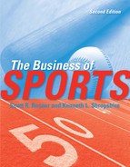
It is well known that professional athletes competing in each of the four major North American sports leagues receive lucrative compensation. In 2008 and 2009, average salaries across these leagues were $5.585 million in the NBA, $3.26 million in MLB, $1.9 million in the NHL, and $1.9 million in the NFL. What is not well known is how these salaries are determined. Professional athletes are often perceived as being overpaid instead of merely well paid. This reflects a misunderstanding of the relevant marketplace for athlete compensation. A comparison of athlete salaries to those of the average person is misleading. Instead, athletes should be regarded as entertainers when it comes to compensation. When considered in this manner, athlete compensation is quite reasonable. Much like entertainers, there is a limited supply of highly skilled athletes who the average person desires to watch either live or on television. This is a signifi-cant reason why athletes (and entertainers) are able to earn such high salaries. (See Table 1 for a list of the average salary growth in each league.)
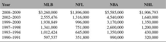
There is, however, an area in which it is fair to compare an athlete’s salary to the average worker’s—the economic justification for how much one is paid. Individuals who are employed in a free and open marketplace are compensated based on their marginal revenue product (MRP); that is, how much the individual employee contributes to the employer’s revenues. Conversely, individuals who are employed in a restricted, uncompetitive marketplace are not compensated based on their MRP. Instead, the employer retains most of the MRP, and the individual is compensated (and some would say exploited) at a more conservative rate. See Table 2 for the top American earners in U.S. sports.
The MRP concept explains why the salaries of professional athletes typically increase with the athletes’ years of experience. A truncated version of the reserve system that set athlete salaries in each league at artificially low rates until the mid-1970s in MLB (and later in other leagues) still exists. Similar to the reserve system that perpetually bound a player to a team at the team’s discretion, each league limits player access to a competitive marketplace for a period of years at the beginning of a player’s career. Not surprisingly, most studies indicate that athletes tend to earn close to the minimum salary established in the league’s collective bargaining agreement during this monopsonistic period. The team captures most of the athlete’s MRP at this stage of his career. After this initial period, the player in each league gains increased but still restricted access to the marketplace (and the full value of the MRP) for a period of years as a result of restricted free agency, salary arbitration, or both. Upon completing this stage, the athlete gains access to the open marketplace via unrestricted free agency. This allows the player to realize close to the full value of his MRP.
In professional sports leagues, the salary of an individual athlete is determined pursuant to the athlete compensation framework established by collective bargaining between the union and management. This determination is typically accomplished through a negotiation between a team and the athlete’s representative. Although the collective bargaining agreement establishes the parameters for this negotiation, the salary for any particular athlete depends on a number of factors both internal and external to that athlete. First, of course, are the factors internal to the athlete, which exist outside of the context of the collective bargaining agreement. The athlete’s skill level, position, experience, injury history, drawing power, and league all impact the compensation earned. A highly skilled, experienced, and seldom-injured athlete playing a “glamour” position in a thriving league will be better compensated than one lacking any of these qualities. In addition, several external factors that are products of the collective bargaining agreement can either increase or decrease athlete salaries. Free agency and salary arbitration increase athlete salaries, whereas a salary cap, luxury tax, and the presence of a reserve system can all decrease athlete salaries. Outside of the collective bargaining agreement, the presence of a competitor league typically leads to dramatic salary increases. These external factors require further elaboration.
Sources: National Football League Players Association, National Basketball Players Association, National Hockey League Players Association, and Associated Press.
As previously mentioned, free agency grants athletes access to a more open marketplace for their services. There are two basic types of free agency: restricted and unrestricted. An athlete is granted restricted free agency after completion of the initial reservation period at the beginning of his career. Restricted free agency provides the athlete whose contract has expired the ability to receive employment offers from other teams in the same league. The athlete’s movement to other teams is restricted, however, because the current employer typically has a right to match the outside offer and maintain the athlete’s services under those exact terms. Alternatively, the team can choose to allow the player to defect and may receive compensation from the new team in exchange for this player. Thus, restricted free agency allows the athlete to obtain a salary increase through the introduction of a quasi-open marketplace. The salary effect is lower if a compensation mechanism is in place, because this places a cost on outside teams that solicit new players. Conversely, the less restrictive the compensation mechanism, the greater the effect of restricted free agency on player salaries.
Unrestricted free agency provides more experienced athletes whose contracts have expired with the opportunity to receive offers from all league teams in an open marketplace. This allows players to receive fair market value for their services. Athlete compensation increases significantly with the arrival of free agent eligibility. It should not be surprising, then, that owners are generally opposed to free agency because of the effects that it has on player salaries. Though now accepted as an essential characteristic of the athlete compensation framework, owners still attempt to impose as limited a system of free agency as possible. However, free agency itself is not necessarily bad for owners. Rather, it is the intersection of free agency with the laws of supply and demand that negatively impacts owners. Unrestricted free agency is not available to every athlete every year. Instead, only those athletes with a particular level of experience whose playing contracts have expired are eligible for free agency. By limiting the number of athletes who are eligible for free agency each year, the supply of players entering the free agent marketplace is artificially lowered. This allows free agents to receive higher salaries than they would in a truly open marketplace where every player is a free agent every year. Doing so would flood the marketplace and depress salaries. So athletes actually have an interest in limiting their access to free agency in order to reap its maximum benefits.
Salary arbitration provides owners and athletes with a method of resolving disputes over the athlete’s salary for the upcoming season while ensuring that the athlete will continue his employment with the team uninterrupted by a holdout over salary. Salary arbitration allows athletes who have completed the initial phase of their careers to compare themselves to other similarly situated athletes in the marketplace in order to obtain salary increases. Athletes have been quite successful in doing so, especially because of the intersection that has occurred between free agency and salary arbitration. The free market effects of free agency have trickled down to the salary arbitration process.
The presence of a competitor league provides athletes with an attractive employment alternative. A new league needs players, the most talented and well known of whom are employed in the established league. These leagues do not abide by their rivals’ collective bargaining agreements. Thus, unencumbered by the established league’s reserve system, all athletes whose contracts have expired are able to gain access to an open marketplace regardless of experience. Historically, the introduction of another bidder for their services has led to a dramatic increase in players’ salaries. Similar to other industries, competition among employers in the labor marketplace benefits the employees—in this case, the athletes.
Over the years, owners have devised various tactics that attempt to depress athlete compensation below competitive levels. The reserve system accomplished this very effectively by perpetually binding a player to a team, thereby preventing him from obtaining a market-level salary. Since the evisceration of the reserve system nearly a generation ago, the collective bargaining process has yielded the development of salary caps and luxury taxes.
Source: Reprinted courtesy of SPORTS ILLUSTRATED: “The Fortunate 50” by Jonah Freedman, August 2, 2010. Copyright © 2010. Time Inc. All rights reserved. With data from “Tiger Tops SI’s List of Top Earners for Sixth Consecutive Year,” SportsBusiness Daily, July 2, 2009.
Notes: *Manning in 2009 has distributed $500,000 in grants through his PayBack Foundation to charities in Indianapolis, near the University of Tennessee (his alma mater), and in his hometown of New Orleans.
Candidates for the U.S. 50 had to be American citizens. SI consulted players associations, tour records, agents, and news reports to compile the list. Endorsement estimates came from Burns Entertainment & Sports Marketing, other sports-marketing execs and analysts, and agents. [Ed. Note: Covers the period from July 1, 2008–June 30, 2009.]
The presence of a salary cap provides a team with a degree of cost certainty in addressing their single highest expenditure—athlete salaries. A salary cap is actually a revenue sharing device for owners and athletes, with the owners guaranteeing the players a significant percentage of certain revenue streams. A hard cap places an absolute limit on this percentage and allows for few exceptions to this limit. A soft cap sets a limit but allows for a number of exceptions.
Another type of cost-containment mechanism is a luxury tax. Rather than limit the amount that each team can pay its players, a luxury tax gives a team a disincentive to exceed paying its players beyond certain salary levels by penalizing them for their excessive spending. This penalty is set at a percentage of the dollar amount of the excess. The higher the percentage and the lower the tax threshold, the greater the disincentive on the team.
The excerpts chosen for this chapter describe all of the aforementioned issues and ideas in great detail. In the first article, Quirk and Fort establish the broad framework for the discussion of athlete compensation. In the next selection, Kahn explains the impact of reserve systems, rival leagues, free agency, and incentives on the labor market for professional athletes. Berri, Brook, and Schmidt analyze the statistical determinants of salary for NBA players in the next selection. Michael Lewis’ bestseller Moneyball brought significant attention to the use of statistical information by teams attempting to gain a competitive advantage, a tactic that has since proliferated not only in baseball but in other sports as well. The reading from Hakes and Sauer examines the economics of this phenomenon in MLB, whereas Bill Gerrard’s excerpt does so in the context of more complex sports that rely on a greater degree of interdependence of players, specifically looking at English professional soccer. The next three readings review provisions of the collective bargaining agreements in North American professional sports leagues that inflate and deflate player salaries. Andrew Healy reviews teams’ inefficient use of the free agency system in MLB, whereas Stephen Yoost examines salary arbitration in the National Hockey League. Richard Kaplan then reviews the deflationary luxury tax system utilized in the NBA since the late 1990’s. In the final article, Duffy reviews the Bosman decision that led to the demise of the reserve system in European soccer and introduction of unfettered free agency, analyzing its impact on the sport throughout the continent.
FRAMEWORK
PAY DIRT: THE BUSINESS OF PROFESSIONAL TEAM SPORTS
James Quirk and Rodney D. Fort
PRO ATHLETES AS ENTERTAINERS
… Unlike unions in most industries, players’ unions do not negotiate “standard wage” policies binding on most or all members. Instead, individual player salaries are determined by direct negotiation between the player and the team owner. Unions do bargain for league-wide minimum salaries, so the changes over time in minimum salaries reflect in part changes in the bargaining power of unions….
While average salary levels are much lower for football and hockey, football (and, to a lesser extent, hockey) also showed marked increases in real salary levels in the 1980s, despite the restrictions on player mobility (free agency) for NFL football relative to baseball and basketball. Thus, in rounding up the usual suspects to explain the real growth in player compensation in all sports, free agency is not the only candidate. Other factors must be at work as well, including the impressive increase in demand for pro team sports tickets, and the striking increase in value of pro sports television rights for all pro team sports…
But the common perception of fans is that pro athletes are wildly overpaid, and that free agency is the culprit. Every red-blooded American boy wants to grow up to be a major leaguer in some sport, and most red-blooded American adult males would toss their careers in a minute if they thought they had a chance to make it in the pros. One example of this sports idolatry can be found in the vastly overinflated assessments that high school athletes make about their chances of turning pro, and, in turn, the similar mistaken perceptions that possess college athletes. Given that many fans would pay for the privilege of playing in the majors (and some actually do pay for the major league experience at adult major league baseball fantasy camps), fans find it a little difficult to accept the fact that pro athletes demand and get salaries in the six- or seven-figure range.
One way to add some perspective to the rise in real salaries for pro athletes is to look at the compensation paid to other entertainers. Perhaps Norby Walters put it best during his 1988 trial for signing college athletes to pro contracts prior to expiration of their college eligibility: “No difference. A sports star is a rock star. They’re all the same.”1 Walters’ insight is right on the mark—star pro athletes are entertainment stars every bit as much as movie and rock stars. The same factors are at work determining the sizes of the big incomes in sports as in other areas of entertainment. These factors are demand by the public for tickets to see stars, the rarity of skilled and/or charismatic individuals with star qualities (in the economist’s jargon, an inelastic supply of talent), and the bargaining power of stars relative to that of the promoters who hire them (team owners in the case of pro sports). In explaining the rise in salaries for sports stars, both increases in the demand for their output and changes in their bargaining power (for example, free agency’s replacing a reserve system) are relevant.
….
In an interesting analogy to the elimination of the reserve clause in baseball, movie entertainers’ earnings skyrocketed with the breakdown of the “contract player” mode of operation in place in the motion picture industry until the 1950s. Studio owners of that era, much as sports team owners today, argued vigorously that the runaway growth in star salaries spelled disaster for their industry. True to predictions, the earnings of movie stars did go up dramatically, but the U.S. motion picture industry remains quite healthy even up to the present time, and is one of the few American industries that has retained its competitive edge in an international setting.
It is interesting that the public perception of the importance of rising salaries for entertainers is so different between movie stars and pro athletes. That star salaries in pop music or the movies cause little public concern is borne out by where news on salaries can be found…. If the level of discussion about salaries in movies and in popular music is a murmur, then it is a high-pitched scream in pro sports….
To fans, the answer to why pro sports are different from other entertainment endeavors is obvious. Other mass entertainment media do not bring philosophers to their defense, lead presidents of the United States to throw out first pitches, or give poets pause to reflect. Whatever the reason, pro team sports are viewed differently from the other mass entertainment industries by almost everyone—fans, sportswriters, players, and owners. But there are some fundamental economic facts of life that apply across the board to all labor markets, including the market for rock stars and pro sports players.
THE WORKINGS OF THE PLAYER MARKET
The market for any labor service, such as the market for the services of pro athletes, follows the good old law of supply and demand and operates on the basis of bids and offers by teams and players. Looking at things from the point of view of any team, we can calculate the most that a profit-oriented team would offer a player; it is the amount that the player would add to the team’s revenue if he were signed. In the jargon of economists, as noted earlier, this is the player’s marginal revenue product, which we will refer to as his MRP. The player’s MRP is the most a team would pay a player because paying a player more than this would decrease team profits; on the other hand, signing a player for anything less than his MRP means that adding the player increases profits for the team.
… George Steinbrenner … was asked once how he decided how much to pay a player. He said, “It depends on how many fannies he puts in the seats.” That was George’s way of saying it depends on the player’s MRP….
From the player’s point of view, the least he would be willing to accept as a salary offer to sign with a team is what he could earn in his next-best employment opportunity (taking into account locational and other nonmonetary considerations). We hesitate to push our luck, but economists refer to this next-highest employment value as the player’s reservation wage. If a team offers a player less than his reservation wage, the player would simply reject the offer and remain employed in his next-best opportunity.
The player’s MRP and reservation wage give the maximum and minimum limits on the salary that a player can be expected to earn. Just where the player’s salary will end up within these limits depends on a number of considerations. Union activities have an impact, especially on players whose reservation wage would have been below the league-wide minimum salary resulting from collective bargaining. The most important consideration is the bargaining power of the player relative to that of the owner. Generally, the more close substitutes there are (that is, the easier he is to replace), the more bargaining power the team has, and the salary will be closer to the player’s reservation wage than to his MRP. The more unique are the skills and drawing power of the player (that is, the tougher he is to replace), the more bargaining power the player has, and the closer the salary will be to the player’s MRP.
Just how far apart the reservation wage and MRP limits on a player’s salary will be depends critically on the negotiating rights for players and owners, built into the player market by the rules of the sport. At one extreme is complete free agency, where the ability of players and owners to negotiate with whomever they choose is unrestricted. At the other extreme is the reserve clause system that operated in baseball until 1976. Under the reserve clause … a player can negotiate only with the team owning his contract. Generally speaking, the more freedom there is for players and owners to negotiate, the closer the minimum (reservation wage) and maximum (MRP) limits on a player’s salary will be. However, there can be substantial remaining bargaining room even under unrestricted free agency.
Suppose first that there is unrestricted free agency, with players and owners free to negotiate with whomever they choose. Under such circumstances, if we ignore locational and other nonmonetary considerations, each player will end up signing with the team to which he is most valuable (the team for which the player has the highest MRP). He will be paid a salary that lies between his MRP with that team, and his MRP with the team to which he is second most valuable (the team to which he has the second-highest MRP). The reason for this is that the team to which the player is most valuable can outbid any other team for the player’s services, and still increase its profits by hiring him. But the team can sign the player only if it offers him at least as much as the player can earn elsewhere (the player’s reservation wage), and the most the player can earn elsewhere is clearly his MRP with the team to which he is second most valuable. In a market with completely unrestricted free agency, if we ignore nonmonetary considerations, the grand conclusion is that the highest salary offered to the player will capture at least his second-highest value in the league, and can be up to (but not exceeding) his highest value in the league.
Under a reserve clause system, the team owning a player’s contract has exclusive negotiating rights to the player. Similarly, the college draft gives the team holding a player’s draft rights exclusive rights to negotiate with him (in baseball, for up to six years…). Instead of a competitive market for the player’s services, under a reserve clause system, there is only one bidder for the player’s services. The highest salary the team holding the player’s contract would be willing to pay the player still is the MRP of the player for that team; but under the reserve clause, there is no competitive pressure on the owner of the contract. As a result, the player’s reservation wage is not bid up to his second-highest MRP in the league. Instead, the player’s reservation wage under a reserve clause system is what the player can earn outside of the league, or the league minimum salary, whichever is higher.
Needless to say, for most athletes, the reservation wage calculated in this way lies far below the player’s value to any team in the league. Under the reserve clause system, a player’s wage will end up some place between his reservation wage and his MRP with the team owning his contract. The reserve clause system lowers the value of the player’s reservation wage by eliminating competing offers by other teams, and, unless the player happens to be under contract with the team in the league to which he is most valuable, the upper bargaining limit has been reduced as well. Predictably, the overall effect of a reserve clause system is to lower player salaries relative to what they would earn under free agency.
Put another way, a reserve clause system acts to direct more of the revenue that a player produces to the team owner than to the player. The effect of unrestricted free agency on a league that previously was under a reserve clause system, as in the case of baseball since 1976, would be a bidding up of player salaries to the point where most of the revenue that is linked to the performance of the team ends up in player salaries. Under a reserve clause system, the team can capture a significant fraction of the revenue linked to a team’s performance, as well as revenue that is not so linked.
For both players and owners, the issue of free agency is critical to their economic well-being. While claims that free agency will destroy pro sports thus far are clearly exaggerated, the division of the monopoly rents created by pro sports certainly is at stake. It should come as no surprise, then, that free agency is the central issue in pro team sports collective bargaining. A secondary collective bargaining concern is the league minimum salary, which under a reserve clause system becomes the reservation wage for most players. Under free agency, the league minimum salary is no longer relevant to regulars, but it remains an important bargaining element for other players not yet eligible for free agency.
The point of all this is that the sports labor market has the same fundamental driving forces as any other labor market, that is, the value produced by an employee and his or her bargaining power, with the wage rate ending up somewhere between the reservation wage and the player’s MRP, and with the player’s MRP depending upon the demand by the public for the sport. Interestingly, what goes on in the player market is often portrayed in the press in exactly the opposite fashion, as though it were changes in player salaries that controlled ticket prices and TV revenues.
TICKET PRICE AND PLAYER SALARIES
Owners of sports teams understandably are concerned about escalating salaries for players. After all, they have to pay the bills. But when owners and league commissioners express their opinions about the level of player salaries in public, they like to come on in their self-appointed role of protectors of the fans. Owners are fond of pointing out that if player salaries increase, they (the owners) will be forced to raise ticket prices, or turn to pay-per-view alternatives, in order to obtain the revenues to pay those salaries. The owners’ line would have it that putting a brake on salary increases really is in the interest of fans, who prefer low ticket prices to high ones. This argument seems to be very effective, because fans typically side with the owners in salary disputes with players and in labor negotiations with player unions….
While the owners get effective mileage from this line, it makes very little economic sense. With some rare classic exceptions, such as Phil Wrigley and Tom Yawkey, owners of sports teams are in the business to make money, or at least not lose money. Nobody has to force an owner to raise ticket prices if he or she is fielding a successful team with lots of popular support and a sold-out stadium. Put another way, even if player costs did not rise, one would expect that ticket prices and TV contract values would rise in the face of increasing fan demand. On the other hand, if the team already is having trouble selling tickets, only sheer folly would dictate raising ticket prices.
Given a team’s roster of players, the simple economic fact of life is that the ticket pricing decision by a profit-oriented owner is completely independent of the salaries paid to those players. Profit-oriented ticket-pricing decisions depend solely on the demand by fans for tickets to the team’s games. The demand for the inputs used to produce the games, including players, is derived from this profit-oriented decision, not the other way around. Ticket prices rise when fan demand rises, which in turn increases player MRPs, which spills over into higher salaries for players.
Nowhere is this logic more clearly evident than in the case of baseball in the period just after the beginning of free agency. Free agency acted immediately to raise player salaries…. But fans would not pay more to watch the same players just because they started earning more. The initial effect of free agency was to lower team profits with little impact on ticket prices…. With few exceptions, ticket prices fell in real terms during the very first years of free agency! Indeed, only the Boston Red Sox and New York Yankees had ticket prices in excess of their 1971 levels as late as 1980, four years after free agency. Thus, salaries rose, but ticket prices did not. Ticket prices prior to free agency were already set by owners at levels representing their best guesses as to what would maximize revenue for their teams. Free agency shifted the bargaining power in the direction of players, and player salaries went up. But changes in player salaries per se had no effect on the demand for tickets and no effect on ticket prices.
… This has been a period of rising demand by the public for the major pro team sports. Rising demand led to increases in both ticket prices and TV contract revenues. In turn, the increased demand for pro sports tickets and TV coverage acted to increase the value of skilled players to teams, that is, their MRPs rose. Then, the bargaining process translated the increased value of player skills into higher player salaries. Salaries continued to grow … for all pro sports, spurred on by the growth in team revenues. Under free agency, as in baseball and basketball, more of the increased revenue goes to players than under a reserve clause system … but salaries go up in either case when demand for the sport increases, and, contrary to the argument of owners, they are the effect and not the cause of higher ticket prices.
It might be that the mistaken perception about the link between player salaries and ticket prices comes from a confusion of two different sources of salary escalation. If a team’s salary bill rises because the team has acquired more expensive talent, then the owner can and undoubtedly will raise ticket prices, not because he or she is paying more in salaries, but because he or she is fielding a more attractive team. That was certainly the case with the Yankees in the early days of free agency…. But looking at the league as a whole, the same group of players was around right after free agency as before, so for an average team, the quality of players didn’t change. Consequently, there was no way that the average owner could pass on to fans the increase in salaries that came with free agency; the salary cost increase came directly out of profits, instead.
THE WINNER’S CURSE
Things are not quite as simple as we have been making them, of course—general managers and scouts really do earn the money they are paid. It is no easy task to predict how a player will perform next season, what his contribution to the team will be, and the size of the crowds the team will draw….
We do not pretend to any such skills. Instead, we assume that the market for players “works” in the sense that, on average, bids by skilled general managers and offers by skilled player agents lead to a situation in which players get paid pretty much according to what we have outlined, that is, what they would be worth in their second-best employment in the league.
Well, actually, they may get a little more than that, and maybe even more than their MRPs to the teams that sign them. There is a well-known phenomenon in bidding theory known as “the winner’s curse,” which might be operative in the player markets of the free agency period….
In a sealed-bid auction, say, for league TV rights, the prospective bidders (the networks and cable systems) each evaluate the revenue potential of the TV rights and then, at a specified time, each in effect submits a dollar bid in a sealed envelope. The “lucky” winner is the individual submitting the highest bid. “Lucky” is in quotes, because, by definition, the winning bidder ends up paying more for the right to televise games, and occasionally much more, than any other bidder was willing to offer. Given that all bidders had access to pretty much the same information about the potential market for TV, this suggests that the winner might well have made a mistake in overvaluing the revenue potential of the contract. This is the “winner’s curse”—winning in a sealed-bid auction means the winner might very well have bid too much, and maybe far too much, for the property. In particular, a measure of how much the winner has overbid is the difference between the winner’s bid and the second-highest bid. In the jargon of the field, this difference is what is “left on the table.”
The free agent market in baseball is not as formal as a sealed-bid auction, but there are problems for a general manager in determining how much a player will be worth to his team and in guessing how much other teams will be willing to offer the player. Ideally, a general manager would like to pay any player just $1 more than the player’s best offer anywhere else, but this option is only available in cases where the team has “right of first refusal,” that is, the right to match any outside offer.
With lots of teams out there operating in the free agent market (and assuming no collusion), there will be vigorous competitive bidding for players. Clearly, teams underestimating the MRPs of free agents will typically not be the teams signing them; instead, there is better chance that the “winners” in the free agent market will be teams overestimating player MRPs, and these are the teams stuck with the “winner’s curse.” And, in turn, the presence of the winner’s curse means that players get paid on average even more than their value in their second-best employment opportunities in the league. This cannot be too surprising. Sportswriters, each year, are fond of rubbing owners’ noses in the winner’s curse by pointing out how overpaid many (some would say most) free agents are, relative to their subsequent performance.
SALARY DETERMINATION IN BASEBALL
Assuming that the baseball player market operates to generate salary offers that correlate roughly with player MRPs, we can identify factors that can be said to “determine” baseball player salaries in the sense that these factors are highly correlated with market-determined salary levels, and thus do a good job of predicting the level of baseball player salaries…. The equation is a “best fit” model of salary determination in the sense that (1) it explains a large portion of the total variation in player salaries, and (2) adding other factors to the equation would not significantly improve its predictive power. Models … are used both by players and by owners in justifying their positions on salary demands in the baseball salary arbitration process….
… The clear conclusion is that income inequality in the rest of the U.S. economy, although high relative to other countries, pales in comparison to the inequality in recent years in baseball salaries.
It is also clear that baseball salaries have become less equally distributed over time, and skewed toward the top of the salary scale, with a noticeable jump between the reserve clause and free agency periods… Overall, from the baseball salary data, we can conclude that while all players benefited from free agency, a disproportionate share of the benefits went to the top players, who were the big gainers from free agency. Players at the lower end of the distribution, still held captive by united mobility for their first six years, lost ground relative to their star teammates.
….
Notes
1. Quoted in Rick Telander, The Hundred Yard Lie, New York: Simon & Schuster 1989, at 41.
THE SPORTS BUSINESS AS A LABOR MARKET LABORATORY
Lawrence M. Kahn
Professional sports offers a unique opportunity for labor market research. There is no research setting other than sports where we know the name, face, and life history of every production worker and supervisor in the industry. Total compensation packages and performance statistics for each individual are widely available, and we have a complete data set of worker–employer matches over the career of each production worker and supervisor in the industry. These statistics are much more detailed and accurate than typical microdata samples such as the Census or the Current Population Survey. Moreover, professional sports leagues have experienced major changes in labor market rules and structure—like the advent of new leagues or rules about free agency—creating interesting natural experiments that offer opportunities for analysis.
….
Of course, it is wise to be hesitant before generalizing from the results of sports research to the population as a whole. The four major team sports employ a total of 3,000 to 4,000 athletes who … earned … far above the … median earnings of full-time, full-year equivalent workers…. But at a minimum, sports labor markets can be seen as a laboratory for observing whether economic propositions at least have a chance of being true….
MONOPSONY AND PLAYER SALARIES
Sports owners are a small and interconnected group, which suggests that they have some ability to band together and act as monopsonists in paying players. The result is that player pay is held below marginal revenue product. I discuss three sources of evidence on monopsony in sports: evidence from the rise and fall of rival leagues, evidence from changes in rules about player free agency, and studies comparing the marginal revenue product of players with their pay. Sports owners have often had monopsony power over players in the sense that in many instances players have the option of negotiating only with one team. Here, salaries are determined by individual team–player bargaining in which marginal revenue product, and the outside options available to teams and players, will affect the outcome. Rules changes and the rise and fall of rival leagues have their effects by changing players’ and teams’ outside options.
RIVAL LEAGUES
There have been two time periods in which rival leagues posed a substantial threat to existing professional sports. The first is the period from 1876 to 1920, when there was a scramble of professional baseball leagues forming, merging, and dissolving. The second is the period from the late 1960s into the early 1980s, when new leagues were born in basketball, hockey, and football.
… Baseball is the oldest major league sport in the United States, beginning with the birth of the National League in 1876. In this early period, there was competition for player services from other baseball leagues. To protect itself against the competition of rival leagues and improve the team owners’ balance sheets, the National League introduced the “reserve clause” in 1879, which meant that players were bound to the team that originally acquired the rights to contract with them. Owners now had additional monopsony power over players, and player salaries dropped.
However, the lower salaries may have contributed to the birth of a new league in 1882, the American Association…. Average nominal National League salaries rose from $1,375 in 1882 to $3,500 in 1891…
This increase in salaries is not conclusive evidence that monopsony power of owners decreased; after all, salaries could have risen for other reasons, like the growth of baseball’s popularity. However, in 1891, four of the American Association teams were absorbed into the National League, and five dissolved AA franchises were bought out by the survivors…. [which coincided with] an abrupt, massive decline in National League player salaries starting in the first season of the merger: player pay fell from $3,500 in 1891 (before the merger) to $2,400 in 1892 to $1,800 in 1893. This pay cut was accomplished as the outcome of the National League owners announcement in 1893 of a new salary policy: the maximum pay for a player was to be $2,400. Indeed, some teams imposed lower caps: eight top players on the Philadelphia Phillies who were all paid more than $3,000 in 1892 found that they were all paid exactly $1,800 in 1893. The sharp decline in player salaries does not appear to reflect a major decline in the demand for baseball entertainment, as attendance climbed through the 1895 season.
The success of the National League waned somewhat in the late 1890s, partly due to a lack of competitive balance, but the baseball market was growing. A new rival league, the American League, began in 1901 with eight teams. It successfully lured many star players from the older league and actually outdrew it in attendance in 1902 by 2.2 million to 1.7 million. In response, the National League attempted to have its reserve clause enforced by state courts to prevent players from jumping leagues; however, because state courts have no jurisdiction for player movements outside a given state, it was ultimately unsuccessful in this effort.
A familiar pattern then emerges. The huge success of the American League brought with it a dramatic rise in player salaries. In fact the salary increase appears to begin in 1900, perhaps reflecting anticipation of the new league. The two leagues merged during the 1903 season, at the end of which the first World Series was played. Then in 1903, salaries in Major League Baseball fell immediately by about 15 percent…. Again, this decline does not seem to reflect any fall in baseball’s popularity that year.
Major League Baseball prospered for the rest of the first decade of the twentieth century, with player costs under control and attendance on the rise. However, attendance fell beginning in 1910, and owners kept a tight lid on salaries. Player discontent resulted in the formation of a union, the Fraternity of Professional Baseball Players of America, at the end of the 1912 season. The owners were under no legal obligation to bargain with a union and reacted to it with some hostility.
This dissatisfaction among players helped pave the way for the Federal League, which was able to recruit to long-term contracts several well-known Major League ballplayers beginning in 1913. The pay cycle began again. While the Federal League was in existence from 1913 through 1915, many players jumped leagues, and major league salaries went from about $3,000 in 1913 to $5,000 in 1915. After the 1915 season, most of the Federal League’s owners were “bought out” in December 1915 by the major leagues, and nominal salaries plummeted back to $4,000 by 1917, a fall that was even larger in real terms due to the inflation of the World War I period.
The Federal League owners who were not part of the settlement pursued an antitrust suit against the settling parties for creating a monopoly; however, this suit was lost in 1922, when the U.S. Supreme Court declared that baseball was not a business.1 This decision began baseball’s antitrust exemption, which was upheld several times, most notably in an unsuccessful attempt by a player named Curt Flood to become a free agent in 1969.2 While Flood lost his case, it may have set the stage for baseball players’ ultimately successful quest for free agency. However, this goal was not achieved through the antitrust laws; in fact, baseball’s exemption lasted with respect to player relations until legislation ending it was passed in 1998. Rather, collective bargaining brought free agency to baseball, as discussed below.
The early experiences of Major League Baseball provide some compelling evidence for the potential impact of monopsony in this labor market. However, the comparisons just discussed all concern baseball, and thus have no real control group. In the modern period, we can use salaries in some sports as control groups for other sports.
From the late 1960s into the 1970s, highly credible rival leagues were born in basketball and hockey. The American Basketball Association (ABA), which lasted from 1967 to 1976, was able to field some very good teams. In 1976, four of its teams were absorbed into the NBA, and these all made the NBA playoffs in several seasons after the merger. The NBA Players Association (NBPA) challenged the merger on antitrust grounds, but then withdrew its lawsuit as the result of a settlement which granted free agency rights to NBA players. The World Hockey Association (WHA), which lasted from 1971 to 1979, also had several excellent teams which were absorbed into the NHL starting in 1979.
The rise and fall of these two rival leagues offer another opportunity to test how monopsony might affect salaries since the other two major team sports—baseball and football—had no such competition in their labor markets until the advent of free agency in baseball in 1976 and the birth of the United States Football League (USFL) in 1982.
… In 1967, there were no rival leagues in baseball, football, or hockey, and the ABA was just getting started. Further, there was no free agency, and players unions had not yet negotiated their first agreements. Thus, the 1967 salaries can be viewed as representing common initial conditions with respect to negotiating rules, although not necessarily with respect to demand conditions.*
By 1970 and 1972, the ABA had been in existence for several years, and NBA players rapidly became the highest paid of the major team sports. The World Hockey Association started in 1971, and by 1972, NHL players outearned football and baseball players by similar margins. These upward movements in the relative salaries of basketball and hockey players, while consistent with effects of the new competition, need to be judged against the changing popularity of these two sports. For example, in the NBA, total attendance rose by 120 percent between 1966–67 and 1971–72, while television revenues went from $1.5 million to $5.5 million during the same period, rises that were much, much greater than the increases for football or baseball during this time…. The shock of higher salaries may also have spurred the teams to market themselves better. Moreover, NBA salaries as a percentage of gross basketball revenues rose from 30 percent in 1967 to 66 percent in 1972, which suggests a structural shift in salary determination that goes beyond a rise in revenues. In the NHL, attendance growth was actually much faster in the five years before the birth of the WHA (135 percent) than while the WHA was in business (7 percent). Thus, the acceleration of NHL salaries after 1971 is telling indeed.
There is one more important example of the impact of a rival league on player salaries, the United States Football League (USFL). Like some of the baseball experiences earlier in the century, the USFL was born out of labor strife in the established league; in this case, it was a seven-week NFL strike in 1982, in which the players had failed to gain any significant ground in their fight for free agency or a share of revenues. From 1982 to 1985, the USFL posed a challenge to the established NFL. The USFL had strong financial backing from such owners as Donald Trump; many NFL players switched leagues; and the USFL was able to sign some high-profile college players such as Anthony Carter and Herschel Walker. However, poor television ratings for the USFL ultimately signaled its demise.
The pattern of football player salaries during the USFL years follows that set by the example of other rival leagues. Real salary increases for NFL players averaged 4 percent per year from 1977–1982, before the USFL, and 5 percent per year from 1985–1989, just after the USFL. In between, real player salary increases were 20 percent per year from 1982–1985. Changes in the popularity of football do not seem sufficient to explain the explosion of salaries during the USFL years. From 1977 to 1981, NFL attendance rose 23 percent, but attendance was actually 2 percent lower in 1985 than in 1981; further, NFL television revenues rose by similar rates before and during the USFL years. Overall, NFL salaries during the USFL period were much higher than could have been predicted on the basis of revenues during that time.†
If one uses other sports as a control group for the experience of football salaries in the USFL years, the same lesson emerges. The salary growth for football players from 1982 to 1985 was 8–10 percentage points per year higher than baseball and basketball, and 17 percentage points per year higher than for hockey players. However, during the 1981–85 period, attendance grew 5 percent in baseball, 11 percent in the NBA, 11 percent in the NHL, and, as noted, fell 2 percent in the NFL; television revenues grew 211 percent in baseball and 35 percent in the NBA, compared to 29 percent in the NFL. The faster growth of NFL salaries during the 1982–85 period despite worse attendance and television revenue increases again suggests the importance of the USFL.
FREE AGENCY
Until 1976, players in each of the four major sports were bound by the reserve clause to remain with their original team, unless that team decided to trade or sell them to another team. They were not allowed to become free agents, who could sell their services to any team.
The path toward free agency started in baseball. The Major League Baseball Players Association (MLBPA) was started in 1952, but it didn’t become a modern union until the former United Steelworkers negotiator, Marvin Miller, took over in 1966. The MLBPA achieved a collective bargaining agreement in 1968, and in 1970 the National Labor Relations Board ordered the parties to use outside arbitrators for resolving grievances. In a farsighted decision, Miller obtained management’s agreement to incorporate the standard player contract, which included the reserve clause, into the collective bargaining agreement. This meant that grievances about the interpretation of this clause were a proper subject for arbitration. In December 1975, an arbitrator ruled that the reserve clause meant that the team could reserve a player for only one year beyond the expiration of any current contract. With the reserve clause in place, almost all teams signed players exclusively to one-year contracts, and so this ruling would have freed virtually all of the veteran players after the 1976 season. The teams, threatened with this possibility, were thus moved to negotiate a formal system of free agency with the union in 1976, calling for free agency (with some relatively minor compensation to any team losing a free agent) for players with at least six years of Major League Baseball service. This provision remains basically in place. In 1994, about 33 percent of players had at least six years’ service. [Ed. Note: In 2009, 308 of the 1,293 players on MLB teams’ 40-man rosters, voluntarily retired lists and disabled lists had at least 6 years of service.]
The rise of free agency in the 1976–77 period had a powerful impact on the salaries of baseball players. The average real increase in baseball salaries was from 0–2 percent per year from 1973–75. In 1976 the average real salary increase was almost 10 percent; in 1977, the first year under the new collective bargaining agreement, 38 percent (!); in 1978, 22 percent, before falling back into single digits growth in 1979. Moreover, baseball salaries as a percentage of team revenues rose from 17.6 percent in 1974 to 20.5 percent in 1977 to 41.1 percent in 1982, further suggesting that free agency has had a structural effect on baseball salary determination.* A final point to note about baseball salary determination is that in a series of grievance arbitration decisions in the 1980s, the owners were found guilty of colluding by not making offers to free agents. This reassertion of cartel wage-setting behavior appeared to be successful in restraining salary growth. Real annual growth in baseball salaries fell from 11 percent in the 1982–85 time period to 3 percent from 1985–87. Moreover, salaries as a percent of revenues fell from about 40 percent in 1985 to 32 percent in 1989 during the collusion period. In 1989, arbitrators levied a $280 million back pay penalty on the owners to be paid out over the 1989–91 period as compensation for the losses imposed by collusion, and salaries as a percent of revenue bounced back to 43 percent by 1991. The collusion episode provides a further illustration of the potential impact of monopsony on salaries.
Basketball players also won free agency in 1976, but by a different route, through the settlement of the players’ antitrust suit challenging the ABA–NBA merger. As a result, free agency in the NBA came on the heels of the ABA–NBA salary war period of 1967–76. Possibly as a result, average salaries grew more slowly in the NBA in the 1977–82 period than in football or baseball, a comparison which does not suggest a major impact of free agency in the NBA in addition to the impact of competition from the ABA. On the other hand, NBA salaries amounted to about 70 percent of revenue in 1977 and “nearly three quarters” in 1983, suggesting some further increase in basketball players’ relative power after the coming of free agency even without the benefit of an alternative league.3 Finally, basketball imposed a salary cap in 1983, and salaries did indeed decelerate after 1985. However, there were many exceptions to the salary cap, and it may ultimately have had little effect on salaries during this period.
EVIDENCE OF THE DEGREE OF MONOPSONISTIC EXPLOITATION
To this point, the argument has relied on presenting abrupt shifts in salaries that are difficult to explain without appealing to the theory of monopsony. An alternative mode of research on salary determination is to compare estimates of players’ marginal revenue products to salaries, and in this way to approximate the degree of monopsonistic exploitation….
… Scully found that star players in 1987 were paid 29–45 percent of marginal revenue product; even though this was the height of the collusion period, the percentage was still much higher than the 15 percent he found for the reserve clause days.4 Zimbalist’s approach compares the players eligible and not eligible for free agency.5 In 1989, for those players with less than three years service, and thus not eligible for salary arbitration or free agency, the ratio of salary to marginal revenue product was just .38 times what it was for those eligible for salary arbitration only and .18 times that for those eligible for free agency.†
These measures of monopsonistic exploitation must be interpreted cautiously since (as noted by the authors of the studies) they do not control for a player’s effects on revenue other than through his own playing statistics’ effects on winning.* However, taken as a whole, this line of research produces additional evidence that making the labor market more competitive leads to higher salaries than would be the case under monopsony. Nonetheless, during the 1980s there still appeared to be widespread monopsonistic exploitation in baseball, and research from this period also showed similar results for basketball.
[Ed. Note: The author’s discussion of the Coase theorem and sports and racial discrimination is omitted. See Chapter 18 for a discussion of the latter topic.]
….
INCENTIVES, SUPERVISION, AND PERFORMANCE
Some of the most intriguing evidence on the links from incentives to performance comes from sports that have not been much discussed to this point, like golf and marathon running. Ehrenberg and Bognanno used data from the 1984 U.S.-based Professional Golf Association (PGA) and 1987 European PGA tours to estimate the impact of incentives on player performance.6 Because the prize structure of a given tournament is known in advance, one can compute the dollar gain to improving one’s finishing position in a tournament. Ehrenberg and Bognanno found that a greater dollar gain to a better finish had a statistically significant favorable effect on a player’s performance, controlling for the player’s ability, his opponents’ ability, and the difficulty of the course. In addition, golfers appear to perform better when it matters more, particularly in the later rounds of a tournament. Finally, golfers’ labor supply, as measured by their propensity to enter a given tournament, is positively affected by the expected gain to participating, implying an upward-sloping labor supply schedule.† However, a more recent replication study, using 1992 PGA data, found that monetary incentives had small and statistically insignificant effects on player performance and that results were sensitive with respect to who rated the weather that prevailed during a tournament.7
The framework devised by Ehrenberg and Bognanno has been used to examine the incentive impact of prize money in two additional sports: marathon running and auto racing.8 In auto racing, Becker and Huselid found that larger monetary rewards to better finishes lowered individual racers’ finishing times and raised the incidence of accidents, presumably due to a greater effort to go fast.9 In marathon races, Frick found that better prize money and performance bonuses for setting records lowered racing times.10
In the major team sports that have been the primary focus of this paper, free agency has brought with it an increased incidence of long-term contracts, a finding Lehn argued was consistent with wealth effects, as players in essence buy long-term income insurance.11 He noted that as the incidence of long-term contracts went from virtually zero during the days of the reserve clause to 42 percent of baseball players with at least two years pay guaranteed as of 1980, the share of baseball players who spent time on the disabled list rose from an average of 14.8 percent from 1974 to 1976 (before free agency) up to 20.8 percent from 1977 to 1980 (the early years of free agency). Lehn surmised that this increase was a moral hazard response by players on guaranteed long-term contract. In this instance, moral hazard refers to a player’s impact on the decision to go or stay on injured reserve.
To perform a sharper test of this hypothesis, he compared players in 1980 who had long-term contracts of three years or more with those who had short-term contracts of two years or less. Prior to signing these contracts, those with long-term contracts were almost two years younger and had 2.2 days per season less disability than those who signed short-term contracts. Thus, those with long-term contracts do not appear to be an especially injury-prone group. Nonetheless, after signing their agreements, those with long-term contracts averaged 12.6 disabled days per season, compared to only 5.2 days for those with 0–2 years. Lehn confirms in a regression setting that this effect is highly statistically significant.12 The finding is strongly suggestive of a moral hazard effect, although one cannot completely rule out that players who had private information that they were fragile were more likely to sign long-term contracts, in which case the results could also reflect adverse selection.
Of course, one way for a team to reduce the moral hazard response is to reward players for not being injured. Lehn notes that 38 out of 155 players with contracts of three or more years, or about 25 percent, had incentive clauses in their contracts.13 These clauses sometimes rewarded either being available to play for most of the season or postseason awards won (such awards typically require being active for all or most of the year). Before signing such long-term contracts, those who ended up with incentive bonuses had virtually identical average propensities to be injured as those without such incentive bonuses. However, after signing, the injured time of players without incentive bonuses was 2.4 times that of those with bonuses. Again, a strong moral hazard response is suggested, although as before, we cannot rule out the adverse selection possibility that players who suspected that they were likely to be fragile have turned down the opportunity to sign a contract with an incentive bonus.
Hiring better quality management is an alternative route, along with contract incentives, for eliciting desired performance levels. In a study of the impact of baseball managers, I estimated the effect of better managers on team and individual player performance.14 Managerial quality was measured by first running a 1987 regression with manager salary as the dependent variable and managerial experience, career winning percentage, and a National League dummy variable as the explanatory variables. Then, using the coefficients from the regression, I plugged in each manager’s actual experience and winning percentage to get a predicted salary level. I then calculated that during the 1969–86 period, hiring a better quality manager significantly raised the team’s winning percentage relative to its past level—even if one also controls for team scoring and runs allowed, suggesting that good managers win the close games. The effect of good managers was even larger when I didn’t control for offense and defense. The latter effect could indicate that better managers are superior judges of talent, or motivate their players, and thus indirectly contribute to offense and defense.
I also studied individual player performance relative to established career levels when the team was taken over by a new manager. The better the quality of the new manager, the better a player’s future performance relative to his past performance. In related calculations, I found an increase in managerial quality more than pays for itself based on Scully’s results for the effect of winning on revenue.15 Because of this, one might have expected the salaries of highly talented managers to be bid up. The fact that they weren’t as measured in the 1987 salary data used in this study may be further indirect evidence of collusion between baseball owners during this time period.
FINAL THOUGHTS
Labor issues in sports may seem distant from the rest of the economy, since they often seem to pit millionaire players against billionaire owners. But while it would be unwise to extrapolate too strongly from the labor market experience of sports, evidence on a particular labor market should not be discounted just because the market has a high profile, either. The strong evidence for monopsony in sports has some parallels to a similar effect that has been found among groups such as public school teachers, nurses, and university professors.16 The evidence from these areas suggests that the phenomenon of employer monopsony power could be more widespread than is commonly acknowledged by economists. The presence of customer discrimination in sports reminds us that there are many sectors in the economy with producer–customer contact where discrimination could persist. The results on player performance suggest that athletes are motivated by similar forces that affect workers in general.
While this paper has concentrated on sports in North America, many of the same economic issues arise in the sports industry elsewhere. Professional soccer leagues in Europe are tremendously lucrative and also must be concerned with player movement and competitive balance…. In fact, European soccer draws more TV revenue than the NBA, Major League Baseball, or the NHL. The promotion and demotion of individual teams to and from a… European superleague involving teams from several countries raise fascinating questions about the role of competitive balance.
….
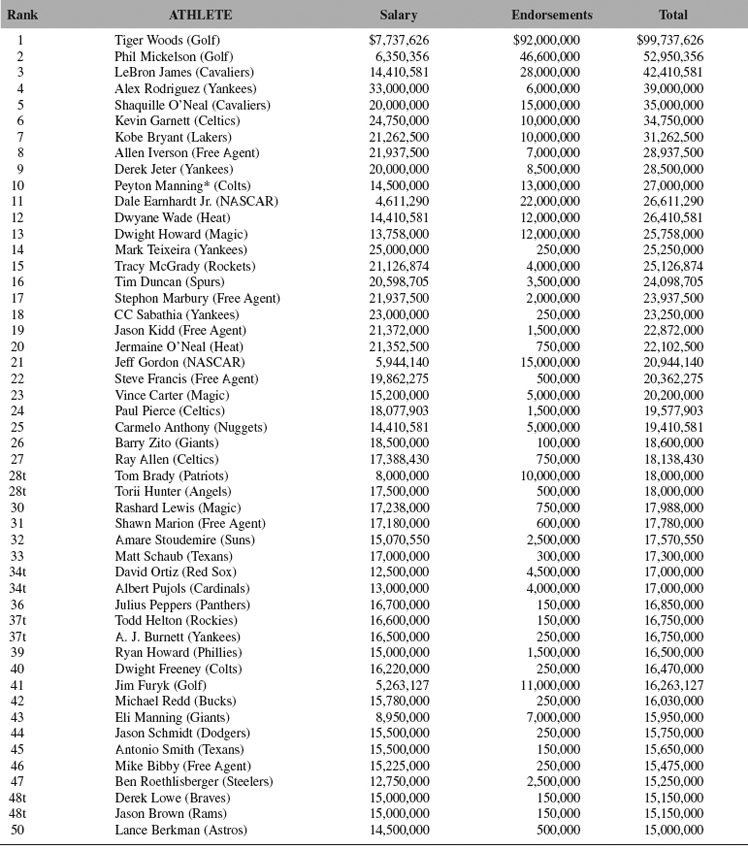
(See Table 3 for salary cap growth in the NBA and NFL.)
Notes
1. Federal Baseball Club of Baltimore, Inc. vs. National League of Baseball Clubs, et al., 259 U.S. 200 (1922).
2. Flood vs. Kuhn, 407 U.S. 258 (1972).
3. Staudohar, Paul D. 1996. Playing for Dollars: Labor Relations and the Sports Business. Ithaca, NY: Cornell University Press, at 108.
4. Scully, Gerald W. 1989. The Business of Major League Baseball. Chicago: University of Chicago Press.
5. Zimbalist, Andrew. 1992. Baseball and Billions. New York: Basic Books.
6. Ehrenberg, Ronald G. and Michael L. Bognanno. 1990. “Do Tournaments Have Incentive Effects?” Journal of Political Economy. 98:6, pp. 1307–1324; Ehrenberg, Ronald G. and Michael L. Bognanno. 1990. “The Incentive Effects of Tournaments Revisited: Evidence from the European PGA Tour.” Industrial & Labor Relations Review. 43:3, pp. 74–88.
7. Orszag, Jonathan M. 1994. “A New Look at Incentive Effects and Golf Tournaments.” Economics Letters. 46:1, pp. 77–88.
8. Ehrenberg, Ronald G. and Michael L. Bognanno. 1990. “Do Tournaments Have Incentive Effects?” Journal of Political Economy. 98:6, pp. 1307–1324; Ehrenberg, Ronald G. and Michael L. Bognanno. 1990. “The Incentive Effects of Tournaments Revisited: Evidence from the European PGA Tour.” Industrial & Labor Relations Review. 43:3, pp. 74–88.
9. Becker, Brian E. and Mark A. Huselid. 1992. “The Incentive Effects of Tournament Compensation Systems.” Administrative Science Quarterly. 37:2, pp. 336–50.
10. Frick, Bernd. 1998. “Lohn und Leistung im Professionellen Sport: Das Beispiel Stadt-Marathon.” Konjunkturpolitik. 44:2, pp. 114–40.
11. Lehn, Kenneth, 1990. “Property Rights, Risk Sharing and Player Disability in Major League Baseball,” in Sportometrics. B. Goff and R. Tollison, eds. College Station, Texas: Texas A&M Press, pp. 35–58.
12. Id.
13. Id.
14. Kahn, Lawrence M. 1993. “Managerial Quality, Team Success and Individual Player Performance in Major League Baseball.” Industrial & Labor Relations Review. 46:3, pp. 531–47.
15. Scully, Gerald W. 1989. The Business of Major League Baseball. Chicago: University of Chicago Press.
16. Ehrenberg, Ronald G. and Robert S. Smith, 2000. Modern Labor Economics, 7th ed. Reading, Mass.: Addison-Wesley.
Table 3 Salary Cap Growth in NBA and NFL
Source: ESPN.com, NFLPA documents, additional data on file from authors.
DOES ONE SIMPLY NEED TO SCORE TO SCORE?
David J. Berri, Stacey L. Brook, and Martin B. Schmidt
“Players must not only have objectives, but know the correct way to achieve them. But how do the players know the correct way to achieve their objectives? The instrumental rationality answer is that, even though the actors may initially have diverse and erroneous models, the informational feedback process and arbitraging actors will correct initially incorrect models, punish deviant behavior, and lead surviving players to correct models.” Douglass North (1994)
INTRODUCTION
The writing of Douglass North lays forth the role instrumental rationality plays in the workings of an efficient market. Given the requirements outlined above and the prevalence of imperfectly competitive industries, one may not expect many markets to be characterized as efficient. A potential exception is the professional sports industry. Unlike most industries, professional team sports have an abundance of information on individual workers and stark consequences for failure. Failure in sports is not only met with a loss of revenues and employment, but public derision via various media outlets. Given the severity of consequences and abundance of information, it is not surprising that economists expect economic actors in professional team sports to follow the dictates of instrumental rationality.
Despite this expectation, there is some research that suggests that instrumental rationality does not always characterize decision-making in professional sports. In baseball we have the “Moneyball” story [see Lewis (2003) and Hakes & Sauer (2006)], or the argument that on-base percentage was under-valued by decision-makers in Major League Baseball. Michael Lewis (2003) told this story primarily with anecdotal evidence in his best-selling book. Hakes and Sauer (2006) confirmed that the empirical evidence was at one point consistent with the Moneyball story. Historically decision-makers in baseball did undervalue on-base percentage.
Turning to the National Football League we see the work of Romer (2006). Romer investigated how often NFL head coaches choose to “go for it” on fourth down and found that coaches were far too conservative. Going for it more frequently would increase the probability that coaches would win games; hence, the actions of the head coaches actually ran counter to their stated objective.
Staying in the NFL we see the work of Massey and Thaler (2006). This work offered evidence of inefficiency in the amateur draft of the National Football League. Specifically, high draft choices were consistently over-valued, in a fashion the authors argue is inconsistent with the precepts of rational expectations.
With respect to professional basketball—the subject of this study—we have the work of Staw and Hoang (1995) and Camerer and Weber (1999). Each of these authors examined the escalation of commitment in the NBA, defined by Camerer and Weber as follows:
“when people or organizations who have committed resources to a project are inclined to ‘throw good money after bad’ and maintain or increase their commitment to a project, even when its marginal costs exceed marginal benefits.” [Camerer and Weber: 59–60]
With respect to the NBA, Staw and Hoang (1995) and Camerer and Weber (1999) investigated the impact a player’s draft position has on playing time. Both of these sets of authors offer evidence that, after controlling for the prior performance of the player, where a player was chosen in the draft still impacts the amount of playing time the player receives after the first two years of the player’s career. Such a finding suggests that NBA decision-makers are slow to adopt new information, maintaining an assessment of a player when the available evidence suggests that the initial perspective is incorrect.
The purpose of this present inquiry is twofold. First we wish to re-examine several pieces of evidence previously presented in the literature. As we will demonstrate, much of this research suggests that decision makers in the National Basketball Association (NBA)—as suggested by the study of escalation of commitment—do not process information efficiently. Our review will be followed by two empirical models. The first will update Berri and Schmidt (2002), which examined the coaches’ voting for the All-Rookie team in the NBA. A second model will ascertain the relationship between player salary and various measures of player productivity. Each of these models—previously described in less detail in The Wages of Wins [Berri, Schmidt, and Brook (2006)]1—will shed light upon the extent information is utilized efficiently in the evaluation of players in the NBA.
THE LESSONS LEARNED
Our story begins with a review of the lessons the current body of literature teaches about the economics of professional basketball. We begin this list of lessons with the story told by a number of published works examining racial discrimination in professional basketball.
Lesson One: Points Scored Dominates the Evaluation of Player Productivity in the NBA
… Berri (2006) surveyed twelve studies examining racial discrimination in the NBA.7 … Given that some papers offered more than one model, Berri’s survey examined fourteen specific models.
Surprisingly, most aspects of player productivity were not consistently linked statistically to the decision-variable examined. In fact, the only factor consistently found to be correlated with player evaluation in the NBA is points scored. In fourteen of the fifteen models examined, points scored was found to be both the expected sign and statistically significant.8 Of the other factors employed by researchers, only total rebounds and blocked shots were statistically significant more often than not.9 The significance of assists was evenly split,10 while field goal percentage was significant in only four of the nine models where it was employed. Every other factor was not significant more than once. In sum, player evaluation in the NBA appears to be driven by points scored and, perhaps, total rebounds, blocked shots, and assists.
Such results tell two important stories. The first centers on the importance of scoring in the NBA. Virtually every study employed a player’s total points or points scored per game.11 One should note, though, that a player’s accumulation of points is dependent on the playing time the player receives and the number of shots taken. Simply staying on the floor and taking a large number of field goal and free throw attempts can lead to the accumulation of lofty point totals. Clearly, efficiency in utilizing shot attempts would also be an indicator of a player’s worth to a basketball team. As noted, though, field goal percentage was not statistically significant in the majority of studies where this factor was considered.12 In other words, a player who scores points can expect to receive a higher salary. Evidence that scoring needs to be achieved via efficient shooting is not quite as clear.
The second story told is about the insignificance of many other facets of a player’s performance. Players do not appear to be evaluated in terms of free throw percentage, steals, or personal fouls. Turnovers, a factor Berri (2009, in press) has identified as significant in determining wins in the NBA, has only been included once and was found to be insignificant. Given the ambiguous results uncovered with respect to everything else besides a player’s points scored per game, these results suggest that a player interested in maximizing salary, draft position, employment tenure, and playing time should primarily focus upon taking as many shots as a coach allows.
Lesson Two: Player Productivity on the Court Creates Team Wins
The literature on team-wins production, though, suggests that wins are about more than points scored per game. We begin this discussion with an obvious statement. The actions of the players on the court determine the outcome of the contest observed. The key to understanding the individual contribution to team wins, though, requires a bit more investigation.
The seminal work of Gerald Scully (1974) provides a guide to those seeking to uncover the relationship between player action and team wins in professional team sports. Scully, in an effort to measure the marginal product of a baseball player, offered a model connecting team wins to player statistics.13
Berri (in press) recently adopted the Scully approach in developing a simple measure of marginal product in professional basketball. This model,14 indicates that points scored, rebounds, steals, turnovers, and field goal attempts each had an equal impact on team wins. Although points scored are important in determining outcomes, factors associated with acquiring possession of the ball also significantly impact a team’s on-court success.
The review of the literature on racial discrimination revealed the importance of points scored, as well as rebounds, blocked shots, and assists. This list of factors can be thought of as highlight variables, since any collection of highlights from the NBA will consists of players scoring points, collecting rebounds, blocking shots, or making creative passes. Although these highlight variables are often correlated with player compensation, wins in the NBA are about more than these highlight factors.
Lesson Three: Team Wins Drive Team Revenue
Perhaps team wins, though, are not the objective of NBA organizations. Such a possibility was considered in the work of Berri, Schmidt, and Brook (2004). These authors examined the importance of winning games as opposed to the star power of a team’s roster. Specifically, a team’s gate revenue was regressed upon team wins, all-star votes received, and a collection of additional explanatory variables. The results indicate that it is wins, not star power, which primarily determines a team’s financial success.
Two anecdotes support this empirical finding. The team who led the league in attendance during the 2003–04 regular season was the Detroit Pistons. Although the Pistons eventually won the 2004 NBA championship, Detroit achieved its success via team defense. Only five teams scored fewer points than the Pistons. Detroit’s regular season scoring leader, Richard Hamilton, ranked only 27th in the league with 17.6 points per game.15
The story of Allen Iverson and the Philadelphia 76ers further supports the low economic value of star power and scoring for an NBA team. In 2005–06 the 76ers sold out every game on the road.16 At home, though, the 76ers were one of only three teams to play before crowds that were less than 80 percent of their home arena’s capacity. Although the 76ers employed a major star and scorer in Allen Iverson, the team’s sub-0.500 record resulted in below average home crowds.
Lesson Four: Team Payroll is not Highly Correlated with Team Wins
Given the abundance of information on player productivity and the expectation that player productivity is linked to player salary, one might expect payroll and wins to be correlated. Stefan Szymanski (2003) investigated the link between wages and team success in a variety of professional team sports, including the NBA. Although the relationship between relative payroll and wins was found to be statistically significant, only 16% of winning percentage in the NBA was explained by relative payroll.17
A similar result was reported by Berri and Jewell (2004). Specifically, a model was offered that looked at the importance of adding payroll, via the addition and subtraction of players, and simply giving existing players an increase in salary. Of these two factors, only adding payroll was statistically significant. Of interest, though, was that the explanatory power of the model employed was only 6%. Much of the changes in team success upon the court in the NBA are not explained by alterations to a team’s level of talent, as measured by additions to team payroll.
Lesson Five: Player Performance is Relatively Consistent Across Time
The lack of a strong relationship between wins and payroll is also observed in Major League Baseball and the National Football League. Berri, Schmidt, and Brook (2006) report that relative payroll in baseball only explains 18% of team wins in MLB from 1988 to 2006. If we look at the NFL from 2000 to 2005 we find that only 1% of wins are explained by relative payroll.18
The inability of payroll to explain wins can at least partially be explained when we look at how difficult it is to project performance in both football and baseball. Berri (2007) and Berri, Schmidt, and Brook (2006) present evidence that performance in football is quite difficult to predict. Summary measures such as the NFL’s quarterback rating, metrics like QB Score, Net Points Per Play, and Wins Per Play—introduced in Berri, Schmidt, and Brook (2006)—and various metrics reported by FootballOutsiders.com tend to be quite inconsistent across time. Less than 20% of what a quarterback does in a current season, measured via any of the above listed metrics, is explained by what a quarterback did last season. A similar result is reported for running backs by Berri (2007).
When we look at baseball we also see a problem with projecting performance. Berri, Schmidt, and Brook (2006) report that less than 40% of what a hitter does in the current season can be explained by what he did last season.19 These results suggest that even if teams were perfectly rational, the inability to project performance is going to result in a weak link between pay and wins.
Although performance inconsistency can explain what we see in the NFL and MLB, in the NBA a different story is told. The aforementioned work of Berri (in press) and Berri, Schmidt, and Brook (2006) detailed a metric called Win Score…
Berri, Schmidt, and Brook (2006) reports that 67% of a player’s Win Score per-minute is explained by what the player did the previous season…. A virtually identical result can be seen with respect to metric reported by the NBA entitled NBA Efficiency.20 … The correlation between NBA Efficiency per minute this season and last season is 0.82.21
These results indicate that player performance in basketball—relative to what we see in football and baseball—is quite consistent. Yet payroll and wins do not have a very strong relationship in the NBA. Hence we need to look for another story beyond inconsistent performance. Before we get to this, though, we need to spend just a moment on one last lesson.
Lesson Six: NBA Efficiency is not About Efficiency
The Win Score metric is based on the statistical relationship between wins and a team’s offensive and defensive efficiency. The estimation of this relationship—reported in Berri (in press) and Berri, Schmidt, and Brook (2006)—reveals that 94% of team wins can be explained by the team’s efficiency metrics. Furthermore, teams tend to average one point per possession. Consequently, factors such as points scored, rebounds, turnovers, steals, and field goal attempts have the same impact, in absolute terms, on team wins.
When we turn to NBA Efficiency we see a similar result. Points scored, rebounds, turnovers, and steals have the same valuation in absolute terms. But rather than consider shot attempts, the NBA’s metric considers missed shots. As a result, an inefficient scorer can increase his value just by increasing his shot attempts.
Consider an NBA player who makes one of the three shots from two-point range. According to NBA Efficiency, his value rises by two from the made shot, and falls by two from the missed shots. So he breaks even. From three-point range he only needs to make one of four to break-even. Most NBA players, though, make at least 33% of their shots from two point range and 25% of shots from beyond the arc. Consequently most NBA players can simply increase their value, according to the NBA’s metric, by simply taking more shots.22
Now consider the story told by Win Score, and the more complex metric introduced by Berri, Schmidt, and Brook (2006), Wins Produced. Both of these metrics note that a field goal attempt uses the team’s possession. For a player to break-even he must make 50% of his two-point shots and 33% of shots from three-point range. Players who fail to shoot efficiently are wasting possessions and hurting a team’s chances to win.
So we have two picture of player performance. Which of these are most consistent with player evaluation in the NBA?
EXAMINING THE ALL-ROOKIE TEAM
To answer this question, let’s first consider voting for the All-Rookie team. Each year the NBA coaches vote for the members on this team. This is the only award—other than the All-Defensive team—that is determined by the NBA’s coaches (as opposed to the media). The voting for this award hence gives us a quantitative measure of the coaches’ evaluation of playing talent.
Berri and Schmidt (2002) examined the voting for this award across four seasons, beginning with the 1994–95 season. Berri, Schmidt, and Brook (2006) updated this analysis with additional seasons. The paperback edition of Berri, Schmidt, and Brook offered a further update, extending the analysis from 1994–95 to 2006–07. It is these empirical results we wish to review.
… The minimum number of voting points a rookie could receive is zero. We considered in our study all rookies who might have received consideration. The sample we chose included all rookies who played at least 12 minutes per game and appeared in 41 contests. In all, 354 rookies were examined. Of these, 21 received the maximum number of votes while 92 were not chosen by any coach.
To explain the variation in this data we considered three variables. The first is player performance (PROD), which can be measured via NBA Efficiency, Wins Produced, points scored, or a collection of player statistics. The other two variables include the initial assessment of a rookie’s value, or his draft position (DFT). We also considered the number of games the rookie played ….
The three estimations… rely upon three different measures of player performance. The first is NBA Efficiency, per game.24 … we see that 73% of the natural log of voting points can be explained by our model. When we turn to Wins Produced per game, a measure highly correlated with team wins,25 we find that only 50% of the variation in voting points can be explained.
What is interesting is that if you turn to a third measure, points scored per game26, we find that we can explain 74% of the variation in voting points. In other words, if we only consider one facet of player performance—scoring—we can explain more of the variation in the coaches’ voting than either of our metrics that summarize much of what a player does on the court….
…. In sum, factors associated with scoring dominate the coaches’ evaluation of rookie performance.
Beyond the statistics, it is interesting that draft position was statistically significant in each estimation of our model. This result suggests that independent of player performance, how a player was viewed on draft night still influences the coaches’ evaluation of a player after an entire year of NBA performance. In other words, like the aforementioned work examining the escalation of commitment, we see evidence that coaches are slow to change their initial assessment of a player.
A TEST OF RECENT FREE AGENTS
One could argue that voting for the All-Rookie team is not indicative of how coaches evaluate talent. It is possible that these votes are not taken seriously and may even be filled in by assistant coaches. Although it seems unlikely that coaches would consistently endorse performances that they know are inferior, one might still wish to see if a more substantive decision suffers from the overemphasis on scoring.
The more substantive decision is the salary paid to free agents….
Beyond simply re-visiting the basic approach in the literature, we also will address a criticism initially noted by Jenkins (1996). Specifically, researchers often regressed current salary upon current player statistics. The NBA, though, often signs players to multi-year contracts. As noted by Berri and Krautmann (2006), for the 2002–03 season, 70% of players labored under a contract that was at least three years in length. More than 14% of the league had a contract that was seven years or longer. Jenkins (1996) argued that to ascertain the relationship between productivity and salary, one must consider measures of productivity at the time the salary is determined.29 In other words, one should restrict the study of salary in professional sports to recent free agents.
Following the lead of Jenkins (1996), we collected data on 255 players who had a multi-year contract begin from the 2001–02 season to 2006–07 campaign. We then constructed a model of player salary… Specifically, we employed as our dependent variable the log of average real salary the player was scheduled to receive over the life of the contract.30 Our choice of independent variables begins with the same collection of performance statistics we employed in our examination of the All-Rookie team. Additionally we considered a number of non-performance factors that might impact player compensation. The first is player injury, which we attempt to capture by considering the number of games played the past two seasons (GP).31 Additionally we consider the size of the market where the player signs (POP).32 Theoretically increases in both games played and market size should lead to larger salaries.
In addition to injury and market size, we also consider the position the player plays. There are five positions in the game of basketball: center, power forward, small forward, shooting guard, and point guard.33 Each of these positions is typically assigned a number, with centers typically listed as a five and the point guard position labeled with the number one. Centers and power forwards are generally taller than guards and small forwards, with many players in excess of seven feet tall. Such height is scarce in the general population, potentially driving up the price of talented front court players. In contrast, quality guards might be in greater abundance, hence driving down the price of these players.34
The final player characteristic we consider is experience (XP), which we incorporate with the number of years played. The guaranteed rookie contracts that first round draft choices receive causes our sample of free agents to generally consist of older players. We suspect that holding performance constant, teams will prefer younger players to older players, so experience should diminish free agent salary.
The final variable we consider is the primary focus of each salary model we have previously noted, the race of the player.
….
As with our examination of the All-Rookie team… first estimated with three different measures of player performance: NBA Efficiency, Wins Produced, and points scored….
All three estimations reveal that market size, playing power forward or small forward, and the race of the player do not impact player compensation. The results with respect to the other non-performance variables were mixed, with both insignificant and significant results reported.
How much of salary we can explain depends on which performance measure we employ. When we utilized NBA Efficiency per game, we can explain 64% of player salary. When we turn to Wins Produced our explanatory power falls to 41%. We can improve upon what we see from Wins Produced when we turn to points scored. When we consider points scored per game as our sole measure of player performance we can explain 59% of a player’s average wage.
What if we turn to the entire collection of player statistics? … [W]hen we utilize the entire vector of player statistics we again find that race is insignificant. We also find that we can explain 64% of player salary, which is the same result we uncovered for NBA Efficiency. Interestingly, beyond points scored, we find that only rebounds and blocked shots statistically impact player compensation. Shooting efficiency, turnovers, steals, assists, and personal fouls do not appear to change the average wage a player commands.
… Once again, it is points scored that have the largest economic impact on player evaluation. A 10% increase in points scored per game increases average salary by 7.7%. A similar increase in rebounds only leads to a 4.8% increase in compensation.
In sum, as we move from a vector of player statistics or the NBA Efficiency model, to a measure of productivity based upon the statistical relationship between player statistics and team wins, our ability to explain player salary declines. Such a result is quite consistent with the argument laid forth in our review of the literature. Player evaluation in the NBA seems overly focused upon scoring. Negative actions, such as inaccurate shooting or accumulating turnovers, do not seem to result in corresponding declines in player compensation.
CONCLUDING OBSERVATIONS
Our review of the literature, as well as our own analysis of the voting for the All-Rookie team and the wages paid to free agents, tell the same story. Players in the NBA need to score to score a major payday.
This was actually the same story told by Glenn Robinson, the first player chosen in the 1994 NBA Draft. Five games into his NBA career the young Glenn Robinson made the following observation: “I expect to do what I’m supposed to do. But a lot of people that don’t know the game, they think it’s all about scoring. I look at it from a team perspective. We have to do well as a team. I don’t need to go out there and score 30 points a game and have us lose. That won’t do us any good. It would help me individually.” Robinson added: “But I want to see all of us get something done.”37
A point similar to Robinson’s observation was also offered by the legendary coach, Red Auerbach.38 From 1950 to 1966, Auerbach guided the Boston Celtics to nine championships, including eight in a row from 1959 to 1966. What was the key to this team’s success? In a biographical sketch posted at ESPN.com it was noted that Auerbach didn’t focus on the individuals on his teams. He looked at the “whole package.” While many of his players were outstanding, the Celtics were the first organization to popularize the concept of the role player. “That’s a player who willingly undertakes the thankless job that has to be done in order to make the whole package fly,” Auerbach said. Auerbach went on to add that the Celtics represent a philosophy that in its simplest form maintains that victory belongs to the team. “Individual honors are nice, but no Celtic has ever gone out of his way to achieve them,” he said. “We have never had the league’s top scorer. In fact, we won seven league championships without placing even one among the league’s top 10 scorers. Our pride was never rooted in statistics.”
Auerbach also bemoaned in an interview broadcast on ESPN Classic that the focus of today’s players is on statistics, as opposed to winning. In Auerbach’s view, Bill Russell was a great player because he didn’t obsess on his own statistics, but rather sacrificed his stats so the team could win. Although Russell averaged only fifteen points per contest, he did grab 22.5 rebounds per game. In other words, although Russell was not much of a scorer, he was an amazing rebounder.
Of course rebounds are a stat. Looking over Auerbach’s comments it appears that when he references statistics, he is talking about scoring. And that appears to be the wisdom of Auerbach: Wins are not just about scoring.
Both Robinson and Auerbach argued that scoring can help individual players, but not necessarily produce wins. Assuming teams and players are trying to win, why does scoring dominate the evaluation process?
In The Wages of Wins a possible answer to this question was provided. Player evaluation in the NBA tends to rely upon visual observation of the player, as opposed to analysis of the numbers. Visual observation would tend to be drawn to the most dramatic event on the court, scoring. Factors such as missed shots and turnovers would not tend to stand out in the mind of the observer. Consequently, these factors tend to be downplayed in the evaluation of players.
Such a story suggests that decision makers need to do more than just possess the necessary information to make the “correct” decision. This information also has to be well understood. Often, though, decision makers have not been trained in the statistical techniques necessary to uncover the statistical relationships necessary for good decision making. As a result, on-base percentage can be undervalued in baseball. NFL coaches can often fail to go for it on fourth down when the data say they should. And finally, scoring can be over-valued in the NBA.
Once again we note that sports have an abundance of information and clear consequences of failure. Yet, decision making in sports has been shown to be inconsistent with the precepts of instrumental rationality. Given this result, we have to wonder: If decision makers in sports are not fully rational, should we expect decision-makers in non-sports industries—where information is less abundant and consequences less severe—to process information efficiently?
Notes
1. This paper was originally presented at the Western Economic Association meetings in 2004 and served as the foundation of chapter 10 of The Wages of Wins. This book did not provide any equations or econometric tables, hence this paper will also serve the purpose of presenting these findings more formally.
….
7. These 12 studies included Kahn and Sherer (1988), Koch and Vander Hill (1988), Brown, Spiro, and Keenan (1991), Dey (1997), Hamilton (1997), Guis and Johnson (1998), Bodvarsson and Brastow (1998, 1999), Hoang and Rascher (1999), Bodvarsson and Partridge (2001), McCormick and Tollison (2001), and Eschker, Perez, and Siegler (2004). With the exception of Hoang and Racher, who considered employment discrimination, and McCormick and Tollison, who considered the allocation of playing time, each study considered the subject of wage discrimination. Kahn and Sherer, in addition to wage discrimination, also presented a model examining the role race played in determining a player’s initial draft position.
8. The term statistical significance is open to interpretation. A common rule of thumb is that the t-statistic should be greater than two. Such a rule, though, could be thought of as too restrictive. Consequently, Berri (2006) argued that a coefficient was only to be considered insignificant in this discussion if its t-statistic falls below 1.5. In other words, an effort was made to increase the likelihood that a variable was significant. Even with this effort, often the non-scoring factors were found to be insignificant.
9. Ten models considered blocked shots and six found this factor to be statistically significant. Eight models considered total rebounds, while seven others broke total rebounds into offensive and defensive rebounds. Total rebounds was statistically significant in five of the eight models. Of those that considered the type of rebound, none found offensive rebounds to be statistically significant. Only one study, McCormick and Tollison (2002), found defensive rebounds to be significant.
10. The ambiguous nature of assists was highlighted in the work of Koch and Vander Hill (1988). These authors found that assists were statistically significant and positive in one regression examining player salary. In another regression, though, assists were statistically significant and negative.
11. Of the studies examining wage discrimination, only Brown, Spiro, and Keenan (1991) considered a player’s per-minute performance. In examining the player draft, Kahn and Sherer (1988) also considered a player’s total accumulation of the statistics employed. Both Hoang and Rascher (1999) and McCormick and Tollison (2001) employed a player’s per-minute production.
12. Six models of wage discrimination considered the impact of field goal percentage. Of these, only the studies that examined the 1985-86 season found shooting efficiency to be both statistically signifi-cant and positively correlated with a player’s salary. This point is highlighted in the work of Bodvarsson and Brastow (1999). These authors tested the same model with data from the 1985-86 and 1990-91 seasons. For the former campaign, field goal percentage is statistically significant. For the latter season, though, it is insignifi-cant.
13. Scully’s approach was also employed by Medoff (1976), Raimondo (1983), Scott, Long, and Sompii (1985), Zimbalist (1992a, 1992b), Blass (1992), and Berri (1999), among others.
14. This model was originally detailed in a working paper by Berri. The appendix to Berri and Krautmann (2006) sketched out the basic idea. In Berri, Schmidt, and Brook (2006) more details were provided. Finally, the original working paper was completed and is scheduled for publication as Berri (in press).
15. Data on team attendance, team scoring, and individual scoring can be found at ESPN.com. Further evidence of the lack of impact from points scored can be found in Berri, Schmidt, and Brook (2006), who report that increases in a team’s points scored per game does not lead to increases in gate revenue in the NBA.
16. This result is consistent with Berri and Schmidt (2006) which reports star power is quite valuable on the road. The NBA does not split regular season gate revenue, so the money a star generates on the road goes to the star’s opponent.
17. Relative payroll is a team’s payroll divided by the league average. Szymanski looked at 1986 to 2000. Berri, Schmidt, and Brook (2006) updated this work via an examination of wins and payroll in the NBA across 15 seasons, beginning with the 1990-91 season and ending with the 2006-07 campaign. For these 15 seasons, relative payroll only explains 10% of team wins.
18. The NFL regression had 190 observations. Relative payroll was also only significant at the 10% level.
19. The metrics considered included OPS (On base percentage Slugging average), SLOB (On base percentage multiplied by slugging average), and Runs produced per plate appearance. Runs produced is calculated via the linear weights measure developed by Thorn and Palmer (1984) and utilized by Blass (1992). Across a sample that began in 1994 and concluded in 2004, only 29% of runs produced per plate appearance were explained by past performance. For OPS and SLOB the explanatory power was 33% and 37%, respectively.
20. The NBA’s efficiency measure is reported at NBA.com. This metric is quite similar to Heeran’s (1992) TENDEX system and Bellotti’s (1993) Points Created model. TENDEX was first formulated by Heeran in 1959. Heeran begins with a model identical to the one currently employed by the NBA, but then weights each player’s production by both minutes played and the average game pace his team played throughout the season being examined. Bellotti’s Points Created model is also quite similar. Bellotti begins with the basic TENDEX model and then simply subtracts 50% of each player’s personal fouls.
21. The result is a sample of 2,836 NBA players from the 1994-95 season through 2003–04.
22. A paperback edition of The Wages of Wins was prepared in 2007. The updated version noted that the critique of NBA Efficiency also applies to the Player Efficiency Rating developed by Hollinger (2002). “In devising his metric Hollinger argued that each two point field goal made is worth about 1.65 points. A three point field goal made is worth 2.65 points. A missed field goal, though, costs a team 0.72 points. Given Hollinger’s values, with a bit of math we can show that a player will break even on his two point field goal attempts if he hits on 30.4% of these shots. On three pointers the break-even point is 21.4%. If a player exceeds these thresholds, and virtually every NBA played does so with respect to two-point shots, the more he shoots the higher his value in PERs. So a player can be an inefficient scorer and simply inflate his value by taking a large number of shots.”
….
24. The NBA Efficiency measure varies depending upon position played. On a per-minute basis, power forwards and centers average between .49 and .50, while small forwards and guards range from 0.41 to 0.43. To overcome this position bias, we calculated a position adjusted NBA Efficiency measure. Specifically we determined each rookie’s per-minute NBA Efficiency value. We then subtracted the average at each position, and then added back the average value for NBA Efficiency across all positions, or 0.45. Once we took these steps, we then multiplied what we had by the number of minutes a player played and divided by games played.
25. As noted by Berri, Schmidt, and Brook (2006) the average difference between team wins and the summation of the Wins Produced by a team’s players is 2.4 from 1993-94 to 2004-05.
26. Like NBA Efficiency per game, points scored per game was adjusted for position played.
27. We took the concept of points-per-shot (PPS) from an article by Neyer (1996). As Neyer explained, this is the number of points a player or team accumulates from its field goal attempts. Its calculation involves subtracting free throws made from total points, and then dividing by field goals attempted. Employing points per shot, rather than field goal percentage, allowed for the impact of three-point shooting to be captured more efficiently.
28. Except for points-per-shot and free throw percentage, all measures were adjusted for position played in a fashion consistent with our adjustment of NBA Efficiency.
29. The work of Jenkins (1996) employed data from the 1980s and 1990s, representing perhaps the longest time period employed in studies of salary discrimination in the NBA. Unfortunately, Jenkins also differed from other works in his choice of player productivity measures. Unlike studies that employed a collection of player statistics, Jenkins followed the lead of professional baseball studies by employing an index of player performance. Hence, we cannot use Jenkins’s work to ascertain the relative importance of points scored, blocked shots, assists, etc.
30. The data on player salary came from USAToday.com: Basketball Salaries Database (http://www.usatoday.com/sports/basketball/nba/salaries/default.aspx). The salary data was converted into constant 2004 dollars.
31. We wish to thank Justin Wolfers for suggesting this variable.
32. Data for U.S. cities was found at the website of the U.S. Census Bureau (http://www.census.gov). Data for Canadian cities was found at Statistics Canada: (http://www.statcan.ca/start.html).
33. Data on player position was taken from various web sites, including ESPN.com. In general, centers and power forwards play closer to the basket and are primarily responsible for rebounds and blocked shots. Point guards and shooting guards play further from the basket and are responsible for ball handling. Small forwards have a mixture of responsibilities.
34. The scarcity of tall people, or “the short supply of tall people” was examined in the work of Schmidt and Berri (2003), Berri et. al. (2005), and Berri, Schmidt, and Brook (2006).
….
37. This was quoted in an Associated Press article written by Jim Litke (1994).
38. The following discussion of Auerbach was first offered at The Wages of Wins Journal (http://dberri.wordpress.com) and also offered in the updated version of The Wages of Wins.
References
….
Berri, D. J. (1999). Who is most valuable? Measuring the player’s production of wins in the National Basketball Association. Managerial and Decision Economics, 20(8), 411–427.
Berri, D. J. (2006). Economics and the National Basketball Association: Surveying the literature at the tip-off. In J. Fizel’s (Ed.) The handbook of sports economics research, (pp. 21–48). Armonk, NY: M.E. Sharpe, Inc.
Berri, D. J. (2007) Back to back evaluation on the gridiron. In J. H. Albert & R. H. Koning’s (Eds.) Statistical thinking in sport, (pp. 235–256). Boca Raton, FL: Chapman & Hall/CRC.
Berri, D. J. (in press). A simple measure of worker productivity in the National Basketball Association. In B. Humphreys & D. Howard’s (Eds.) The business of sport. Westport, CT: Praeger.
….
Berri, D. J., & Jewell, T. (2004). Wage inequality and firm performance: Examining a natural experiment from professional basketball. Atlantic Economic Journal, 32(2), 130–139.
Berri, D. J., & Krautmann, A. C. (2006). Shirking on the court: Testing for the incentive effects of guaranteed pay. Economic Inquiry, 44, 536–546.
Berri, D. J., & Schmidt, M. B. (2002). Instrumental vs. bounded rationality: The case of Major League Baseball and the National Basketball Association. Journal of Socio-Economics, 31(3), 191–214.
….
Berri, D. J., Schmidt, M. B., & Brook, S. L. (2004). Stars at the gate: The impact of star power on NBA gate revenues. Journal of Sports Economics, 5(1), 33–50.
Berri, D. J., Schmidt, M. B., & Brook, S. L. (2006). The wages of wins: Taking measure of the many myths in modern sport. Palo Alto, CA: Stanford University Press.
….
Camerer, C. F., & Weber, R. A. (1999). The econometrics and behavioral economics of escalation of commitment: A re-examination of Staw and Hoang’s NBA data. Journal of Economic Behavior and Organization, 39, 59–82.
….
Football Outsiders. Method to our madness. Retrieved February 2007, from http://www.footballoutsiders.com/methods.ph.
….
Hakes, J. K., & Sauer, R. D. (2006). An economic evaluation of the Moneyball hypothesis. Journal of Economic Perspectives, 20(3), 173–185.
….
Jenkins, J. A. (1996). A re-examination of salary discrimination in professional basketball. Social Science Quarterly, 77(3), 594–608.
….
Lewis, M. (2003). Moneyball: The art of winning an unfair game. New York, NY: W.W. Norton & Company.
….
Massey, C., & Thaler, R. (2006). The loser’s curse: Overconfidence vs. market inefficiencies in the National Football League draft. Unpublished paper.
….
North, D. (1994). Economic performance through time. American Economic Review, 84(3), 359–368.
….
Romer, D. (2006). Do firms maximize? Evidence from professional football. Journal of Political Economy, 114(2), 340–365.
….
Scully, G. W. (1974). Pay and performance in Major League Baseball. American Economic Review, 64(6), 917–930.
….
Staw, B. M., & Hoang, H. (1995). Sunk costs in the NBA: Why draft order affects playing time and survival in professional basketball. Administrative Science Quarterly, 40(3), 474–494.
….
Szymanski, S. (2003). The economic design of sporting contests. Journal of Economic Literature, XLI(4), 1137–1187.
….
AN ECONOMIC EVALUATION OF THE MONEYBALL HYPOTHESIS
Jahn K. Hakes and Raymond D. Sauer
In his 2003 book Moneyball, financial reporter Michael Lewis made a striking claim: the valuation of skills in the market for baseball players was grossly inefficient. The discrepancy was so large that when the Oakland Athletics hired an unlikely management group consisting of Billy Beane, a former player with mediocre talent, and two quantitative analysts, the team was able to exploit this inefficiency and outproduce most of the competition, while operating on a shoestring budget.
The publication of Moneyball triggered a firestorm of criticism from baseball insiders (Lewis, 2004), and it raised the eyebrows of many economists as well. Basic price theory implies a tight correspondence between pay and productivity when markets are competitive and rich in information, as would seem to be the case in baseball. The market for baseball players receives daily attention from the print and broadcast media, along with periodic in-depth analysis from lifelong baseball experts and academic economists. Indeed, a case can be made that more is known about pay and quantified performance in this market than in any other labor market in the American economy.
In this paper, we test the central portion of Lewis’s (2003) argument with elementary econometric tools and confirm his claims. In particular, we find that hitters’ salaries during this period did not accurately reflect the contribution of various batting skills to winning games. This inefficiency was sufficiently large that knowledge of its existence, and the ability to exploit it, enabled the Oakland Athletics to gain a substantial advantage over their competition. Further, we find that, even while various baseball interests denounced Beane and Lewis as charlatans in a stream of media reports, market adjustments were in motion (for discussion, see Lewis, 2004; Craggs, 2005). These adjustments took place around the time Lewis’s book was published, and with sufficient force that baseball’s labor market no longer exhibits the Moneyball anomaly.
Because sports often embody situations where choices are clear and performance and rewards are measurable, they generate useful conditions for studying the behavior of market participants. There are many examples. McCormick and Tollison (1986) use variation in fouls from basketball games to illustrate how the likelihood of punishment affects crime. Brown and Sauer (1993a, 1993b) used point spreads for professional basketball games to consider the influence of psychology and information on market prices. Studies find that the behavior of soccer players conforms well with game-theoretic predictions of equilibrium behavior in penalty kick situations (Chiappori, Levitt and Groseclose, 2002). Moreover, in laboratory experiments that are analytically similar to penalty kick situations (but not described in a soccer context) soccer players act as predicted, whereas students from the general population do not, highlighting the relevance of experience in natural settings to results in the lab (Palacios-Huerta and Volij, 2006).
The present paper depicts a particularly clear case of mispricing in the baseball labor market, accompanied by successful innovation and subsequent adjustment in market prices. Although reasons for the failure of efficient pricing are not fully understood, it seems clear that the correction in market prices was tied to the diffusion of knowledge, as competing franchises mimicked the Athletics’ strategy, in part by hiring Beane’s chief assistants away from the Oakland organization.
MEASURES OF OFFENSIVE PRODUCTIVITY IN BASEBALL AND THEIR CONTRIBUTION TO WINNING
Measures of Batting Skill
A Major League Baseball game consists of nine scheduled innings, in which each team has an opportunity to score runs on offense in its half of each inning. The team on offense is limited to three outs per inning, after which play and scoring cease. Play then resumes with the opponent taking its turn at bat. The limit on outs is crucial. Scoring runs is the objective of the team at bat, and this is accomplished by a combination of skills: in particular, skill at hitting the ball and the ability to avoid making an out.
The most common measure of batting skill is the batting average, which is the ratio of hits to total at-bats. The batting average is a crude index. By weighting singles and home runs the same, it ignores the added productivity from hits of more than a single base. Much better is the slugging percentage, which is total bases divided by at-bats, so that doubles count twice as much as singles, and home runs twice as much as doubles.
Nevertheless, both the batting average and slugging percentage ignore potentially relevant dimensions of batter productivity. When baseball statistics are calculated, sacrifices and walks are not counted as official at-bats, and so they do not figure into either batting average or slugging percentage. In particular, since a fundamental element of batting skill is the ability to avoid making an out, the failure to account for walks is a serious omission. Hitting a single leads to a higher batting average, and receiving a walk doesn’t show up in batting average, but in both cases the batter ends up at first base. The statistic that takes walks into account is called on-base percentage, which is defined as the fraction of plate appearances (including both official at-bats as well as walks) in which the player reached base successfully through either a hit or a walk.
Members of the Society for American Baseball Research (SABR) have studied a variety of combinations of on-base percentage and slugging percentage in the hope of generating a single statistic that will capture a batter’s contribution. It has long been known among this group, dubbed sabermetricians, that linear combinations of these two percentages are very highly correlated with runs scored, the primary objective of an offense. The essence of the Moneyball hypothesis is that the ability to get on base was undervalued in the baseball labor market.
Contribution to Winning
We use linear regression analysis to confirm that on-base percentage is a powerful indicator of how much a batter contributes to winning games. In Table 4, the dependent variable in the regression is the team’s winning percentage. The data for these calculations are performance data over five seasons from 1999 to 2003. Column 1 of Table 4 shows that looking only at a team’s own on-base percentage and the on-base percentage of its opponent can explain 82.5 percent of the variation in winning percentage. Column 2 shows that looking only at a team’s own slugging percentage and the opponent’s slugging percentage can explain 78.7 percent of the variation in winning percentage. Column 3 incorporates both measures of batting skill, which improves the explanatory power of the regression to 88.5 percent of variance. The coefficients on skills for a team and its opponents are quite close to each other, as would be expected in a two-sided symmetric game.1 This is to be expected given the well-documented high correlation between runs scored and linear combinations of on-base and slugging percentage.
The final column of Table 4 is used to assess Moneyball’s claim (Lewis, 2003, p. 128) that, contrary to then-conventional wisdom, on-base percentage makes a more important contribution to winning games than slugging percentage. To facilitate the comparison, the “on-base” and “on-base against” coefficients are restricted to be the same, as are the “slugging” and “slugging against” coefficients. The coefficients in this regression for on-base percentage are more than twice as large as the coefficients for slugging, which supports Lewis’s claim. A one-point change in a team’s on-base percentage makes a significantly larger contribution to team winning percentage than a one-point change in team slugging percentage
Table 4 The Impact of On-Base and Slugging Percentage on Winning
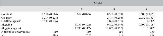
Source: Journal of Economic Perspectives. Used with permission.
Notes: Data are aggregate statistics for all 30 teams from 1999–2003. Coefficient estimates were obtained using ordinary least squares. Coefficients for annual 0/1 dummy variables are suppressed. Standard errors are in parentheses. Superscript “R” indicates that the coefficient was restricted to equal its counterpart in the regression. The p-value for the null hypothesis that restrictions are valid is 0.406 (F = 0.52).
THE LABOR MARKET’S VALUATION OF SKILL AND THE ATHLETICS’ MANAGEMENT STRATEGY
Wages in Major League Baseball
We now turn to the question of the labor market’s valuation of batting skills…. during the five seasons spanning 2000–2004. The average wage for position players increased over the sample period, from $2.56 million to $3.32 million, with the figure for 2004 slightly lower than the prior year. Home run hitters, defined as those with more than 25 homers in a season (roughly one standard deviation above the mean), earn $3 million to $4 million more than the average player.
Valuation of Batting Skill in Baseball
An efficient labor market for baseball players would, all other factors held constant, reward on-base percentage and slugging percentage in the same proportions that those statistics contribute to winning. We assess this proposition by estimating earnings equations for position players (which means that we exclude pitchers) for the 2000–2004 seasons.
….
Relative to younger players who have limited ability to negotiate their pay, players who are eligible for arbitration earn more, with an additional increment for players eligible to become free agents. We also obtain positive and statistically significant returns to expected playing time. The returns to on-base percentage and slugging are both positive, as expected. However, the coefficient for slugging on the income of a player is considerably larger than the coefficient for on-base percentage, which is the reverse of their importance to team success. This is consistent with Moneyball ’s claim that on-base percentage is undervalued in the labor market.
….
A sense of the absolute magnitude of the premium for sluggers can be obtained for each year by evaluating the effect on salary of one-standard-deviation increases in slugging percentage and on-base percentage…. The incremental salary impacts for slugging percentage in the first four years range from $0.52 million to $0.70 million and are three to four times as large as the incremental impact of a standard deviation increase in on-base percentage.
This finding contrasts with the evidence… which indicates that swapping a small increment of slugging percentage in return for a small increment of on-base percentage would increase a team’s winning percentage. The lack of a market premium for hitters with superior skill at the patient art of reaching base through walks validates the systematic approach taken by the Oakland Athletics in identifying such players, and thereby winning games at a discount relative to their competition.
The relative valuation of on-base and slugging percentage is abruptly reversed for the year 2004—and this result exists despite the inertia produced by long-term contracts. The salary returns to slugging are similar in 2004 to prior years, but 2004 is the first year in which on-base percentage becomes statistically significant. The labor market in 2004 appears to have substantially corrected the apparent inefficiency in prior years… and the ratio of the monetary returns to reaching base and slugging is very close to the ratio of the statistics’ contributions to team win percentage.
We have thus verified a central claim in Moneyball by showing that on-base percentage was undervalued at the beginning of the 2000–2004 period in Major League Baseball. There are two obvious caveats which should be addressed before accepting Lewis’s argument completely. First, it might be that fans prefer watching sluggers, and that the allegation of mispricing confuses the ability to “win ugly,” but unprofitably, with profit maximization. Second, the analysis thus far does not link the Oakland A’s success to an explicit strategy capitalizing on the alleged mispricing of skill. We turn to these questions now.
Efficiency and Management Strategy in the Oakland A’s Personnel Decisions
The Oakland Athletics’ management strategy, as reported by Lewis (2003, p. 124) was to minimize the payroll required to build a team which would successfully contend for a playoff spot…. [A] scatterplot of team salaries and winning percentage … demonstrates the Athletics’ ability to win “on the cheap.” Because Major League Baseball salaries were increasing rapidly during this period, each team payroll is indexed to the league-wide average for that season….
Other teams along the “frontier” of efficiently converting payroll into wins usually either failed to have enough on-field success to make the playoffs (like the 2003 Tampa Bay Devil Rays, 2000 Florida Marlins and 2001 Minnesota Twins), or, like the 2001 Seattle Mariners, were far better on the field than their nearest competition during the regular season. As the baseball labor market corrected in 2004, the Athletics remained near the frontier of salary efficiency, but their advantage was narrowed. Despite increasing their payroll to 86 percent of league average, they finished just behind the California Angels (now called the Los Angeles Angels of Anaheim) in 2004, missing the playoffs for the first time since 1999.
In effect, the A’s were able to purchase a successful team less expensively by focusing on players with a higher on-base percentage, chiefly players who excelled at receiving walks. Disciplined hitters avoid swinging at balls, forcing a pitcher to throw strikes to get an out. A team of disciplined hitters is rewarded in several ways. More walks occur, raising on-base percentage. A reputation for discipline causes pitchers on the other team to throw more pitches in the strike zone, which are easier to hit. Finally, patient hitters cause pitchers to throw a greater quantity of pitches, which raises the chance that a tiring pitcher will start to throw pitches that are easier to hit successfully.
The emphasis on taking walks is apparent in the Oakland A’s aggregate batting statistics. They led the American League in walks in 1999 and 2001, were second or third in 2000, 2002 and 2004, and fifth in 2003 (as shown at http://www.baseballreference.com/leagues/AL.shtml). Coupled with the emphasis on walks in player development, this success suggests that an explicit strategy was being followed.
Although the interpretation … treats player skills as strictly fixed, observed skill is a combination of innate skill with team investment in player development. The A’s strategy was carried out both in signing players and in coaching. In signing position players, Oakland looked for hitters who did not appear outstanding in batting average or slugging percentage, and thus who commanded only moderate salaries, but who made a substantial contribution to winning baseball games when on-base percentage and the ability to draw walks were taken into account. At the same time, the Oakland coaching staff preached the virtues of disciplined hitting and not swinging at bad pitches (or even at certain strikes that cross the plate in a way that would be hard to hit solidly). Third baseman Eric Chavez said: “The A’s started showing me these numbers … how guys’ on-base percentages are important. It was like they didn’t want me to hit for average or for home runs, but walks would get me to the big leagues” (Lewis, 2003, p. 151). Miguel Tejada, who won the 2002 American League Most Valuable Player Award, was quoted as saying (presumably half-joking): “If I don’t take twenty walks, Billy Beane send me to Mexico.”
Personnel movements during these years illustrate that the Athletics were able to substitute new players to maintain team success when individual players became too expensive to keep. As one example, the A’s had a player named Jason Giambi who won the Most Valuable Player award in the American League in 2000 for his hitting prowess. After the 2001 season, Giambi had enough major league experience to qualify for free agency. After making $4.1 million in 2001, Giambi signed a seven-year contract with the New York Yankees for $120 million dollars. Oakland made no serious effort to match this offer. However, by signing inexpensive players to replace the lost superstar with incremental improvements across several positions, the Athletics repeated as division champions in 2002, actually improving their season record by one win. The replacement of offensive production from a now expensive Jason Giambi with an array of undervalued talent—notably high on-base percentage hitters Scott Hatteberg and David Justice—neatly encapsulates Lewis’s argument, and ours.
Winning the Oakland A’s Way and Profit Maximization
Although a comprehensive analysis of revenues and costs for the Oakland franchise is beyond the scope of this paper, suggestive evidence is readily available that is consistent with the Athletics’ strategy being both an on-field and financial success…. In 1995, new ownership dismantled the team roster to cut costs, and performance declined. The low-budget strategy centering on on-base percentage was put in place at this time (Lewis, p. 58), and performance began to improve in 1999…. [T]he A’s revenues were sensitive to performance: attendance increased sharply while average ticket prices rose as on-field success improved. Thus, while the Oakland organization focused on winning games cheaply, their improved performance increased demand. The evidence… is fully consistent with our view that the Oakland strategy for winning games was a successful exploitation of a profit opportunity.
CONCLUDING REMARKS
Our analysis supports the hypothesis that baseball’s labor market was inefficient at the turn of the twenty-first century. Arguably, this mispricing of skill had been present for a sustained period of time, perhaps decades. Dodgers General Manager Branch Rickey—perhaps best-known for breaking the color barrier in baseball with Jackie Robinson—argued in print for the importance of on-base percentage during the 1950s, but he failed to win converts (Rickey, 1954; Schwartz, 2004, p. 59). Bill James, a pioneer among sabermetricians, published a series of statistical analyses of scoring beginning in the late 1970s, and came to a similar conclusion (Lewis, 2003, pp. 76–77; James, 1982).
Consistent with the vociferous objections of baseball insiders to the possibility that quantitative analysis could help guide team management, the sabermetric insights of Rickey, James and others were apparently ignored. James in particular grew frustrated that his careful work was dismissed by the game that was his passion: “‘When I started writing I thought if I proved X was a stupid thing to do that people would stop doing X,’ he said. ‘I was wrong’” (Lewis, 2003, p. 93).
Apparently only Oakland executive Sandy Alderson read, absorbed and incorporated Bill James’s analysis into an explicit organizational strategy (Lewis, 2003, p. 63, p. 142). To execute the strategy, Oakland reached outside baseball circles and hired two young Ivy League graduates with quantitative backgrounds to evaluate personnel.
Oakland’s on-field performance, combined with their radical low-budget approach, exposed a flaw in the way personnel decisions were made in baseball. Once exposed (with the help of Lewis’s best-seller), competitive forces were set in motion as teams sought to replicate or improve upon the A’s formula. Oakland’s competitors sought success by attempting to hire the personnel management team assembled by Alderson. The two Ivy Leaguers mentioned above were hired as General Managers (that is, as executives with authority over personnel decisions) by the Toronto Blue Jays and the Los Angeles Dodgers during and after the 2003 season (Saraceno, 2004). Although the Boston Red Sox failed in their attempt to hire both the Athletics’ General Manager (Billy Beane) and Assistant General Manager, they followed Beane’s advice by hiring the similarly inclined Theo Epstein, making him the youngest General Manager in baseball history (Shaughnessy, 2003). In addition, the Red Sox hired the dean of sabermetrics, Bill James himself, in an advisory capacity. The Red Sox proceeded to win the World Series in 2004.
This diffusion of statistical knowledge across a handful of decision-making units in baseball was apparently sufficient to correct the mispricing of skill. The underpayment of the ability to get on base was substantially if not completely eroded within a year of Moneyball’s publication.
Notes
1. Similar results are obtained using a team’s Earned Run Average, a measure of the runs given up by a team’s pitchers, as a measure of the quality of a team’s pitching and its defensive ability.
References
Brown, William O. and Raymond D. Sauer. 1993a. “Fundamentals or Noise? Evidence from the Basketball Betting Market.” Journal of Finance. September, 48:4, pp. 1193–1209.
Brown, William O. and Raymond D. Sauer. 1993b. “Does the Basketball Market Believe in the Hot Hand: Comment.” American Economic Review. December, 83:5, pp. 1377–86.
Chiappori, Pierre-Andre´, Steven Levitt and Timothy Groseclose. 2002. “A Test of Mixed Strategy Equilibria: Penalty Kicks in Soccer.” American Economic Review. September, 92:4, pp. 1138–51.
Craggs, Tommy. 2005. “Say-It-Ain’t-So Joe.” SF Weekly. July 6. Available at http://www.sfweekly.com/Issues/2005-07-06/news/feature.html.
James, Bill. 1982. The Bill James Baseball Abstract 1982. New York: Ballantine Books.
….
Lewis, Michael. 2003. Moneyball: The Art of Winning an Unfair Game. Norton: New York.
Lewis, Michael. 2004. “Out of Their Tree.” Sports Illustrated. March 1.
McCormick, Robert E. and Robert D. Tollison. 1984. “Crime on the Court.” Journal of Political Economy. April, 92:2, pp. 223–35.
Palacios Huerta, Ignacio and Oscar Volij. 2006. “Experientia Docet: Professionals Play Minimax in Laboratory Experiments.” NajEcon Working Paper Reviews No. 122247000000001050. Available at: http://www.najecon.org/naj/v12.htm.
….
Rickey, Branch. 1954. “Goodbye to Some Old Baseball Ideas.” Life Magazine. August 2. Reprinted at http://www.baseballthinkfactory.org/btf/pages/essays/rickey/goodby_to_old_idea.htm.
Saraceno, Joe. 2004. “Dodgers Turn to Ivy League,” USA TODAY, March 17.
Schwartz, Alan. 2004. The Numbers Game: Baseball’s Lifelong Fascination with Statistics. New York: Thomas Donne Books, St. Martin’s Press.
Shaughnessy, Dan. 2003. “Beane Has Looked Sharp By Doing Things His Way.” Boston Globe. September 28.
IS THE MONEYBALL APPROACH TRANSFERABLE TO COMPLEX INVASION TEAM SPORTS?
Bill Gerrard
INTRODUCTION
Michael Lewis’ bestseller, Moneyball: The Art of Winning an Unfair Game (2003), tells the story of how the Oakland Athletics in Major League Baseball (MLB) have achieved a sustained competitive advantage over an eight-year period despite being one of the lowest wage spenders. At the core of the Moneyball story is the systematic use of player performance data to guide player recruitment, player valuation, and field tactics as championed by Oakland’s general manager, Billy Beane. Moneyball has attracted an international audience and, inevitably, raised questions on the extent to which the approach of the Oakland A’s can be replicated in other team sports. For example, the transferability of Moneyball to association football (i.e., soccer) featured recently as the cover article in a leading UK sports monthly (Runciman, 2007).
The objective of this paper is to explore the degree to which Moneyball represents transferable knowledge. Specifically, the paper poses the question: Can Moneyball be transferred to complex invasion team sports such as the various codes of football? It is argued that atomistic striking and fielding team sports such as baseball are most conducive to the systematic exploitation of player performance data because of the high degree of separability of individual playing contributions. However, the approach can be applied in more complex invasion team sports. This is illustrated with a benchmarking analysis of team performance in English Premiership soccer.
The structure of the paper is as follows. The following section provides a statistical analysis of the Moneyball effect, measuring the magnitude of Oakland’s competitive success over the period of time since Billy Beane’s appointment as general manager in 1998. The results of benchmarking using both structural regression models and payroll costs per win are presented. The next section analyzes Oakland’s knowledge-based “David” strategy that involves utilizing the insights of the statistical analysis of baseball data (i.e., sabermetrics). The following section discusses the difficulties in moving beyond atomistic striking and fielding team sports to apply Moneyball to more complex invasion team sports such as soccer. The application section illustrates the application of statistical performance analysis to English Premiership soccer over a four-year period and attempts to differentiate strategically between the alternative approaches of the two most successful teams. The conclusion section offers some thoughts on the barriers to the transferability of Moneyball to other team sports.
OAKLAND A’S: MEASURING THE MONEYBALL EFFECT
Moneyball: The Art of Winning an Unfair Game (Lewis, 2003) provides an account of how the Oakland A’s have consistently been contenders for the postseason playoffs in the MLB in recent years despite having one of the lowest payroll budgets in the league. The turnaround from a low-budget, low-achievement team to a low-budget, high-achievement team began in 1998 with the appointment of a former player, Billy Beane, as general manager. Moneyball is the Billy Beane story…. [T]he turnaround has been truly remarkable. In his first season in charge, Beane’s Oakland team posted a losing regular season with a win ratio of .457, which ranked 21st out of 30 teams. But even this marked a significant achievement since Oakland ranked as the third lowest payroll spenders in 1998. Every season since 1998 has been a winning season [Ed. Note: The A’s subsequently posted losing seasons in 2007, 2008, and 2009.] but Oakland has remained one of the lowest spending teams with 2004 as the only year in which Oakland’s payroll expenditure was ranked above the lowest third.
Seasons 2001 and 2002 are the principal focus of Moneyball. In both seasons Oakland had the second highest regular-season win ratio winning in excess of 100 games (in a regular-season schedule of 162 games) yet were the second lowest payroll spenders in 2001 and third lowest in 2002. The scale of Oakland’s achievement can only be properly appreciated if compared with the record of the MLB’s goliath, the New York Yankees, over the same period…. Oakland has trailed the Yankees most seasons in terms of games won but the gap has been relatively small. Over the eight seasons from 1999-2006, the Yankees have averaged 3.9% more wins per season than Oakland (i.e., just over six wins). Yet over the same period the Yankees outspent Oakland by a factor of 3.22. In other words a 216.7% payroll premium has yielded only a 3.9% win advantage. And indeed in 2000 and 2002 Oakland returned a higher win ratio than the Yankees. (See Table 5.)
The Yankees represent an extreme case of a high-budget, high-achievement team. A fuller evaluation of the extent of the Moneyball approach requires a benchmarking analysis of Oakland’s pay and performance record against all of the other MLB teams since 1998. There are two basic methods of quantitative performance benchmarking. The simplest method is to use ratio analysis to calculate the efficiency of an organization in terms of output per unit of input. Ratio analysis has the advantage of simplicity and transparency, allowing a direct comparison of organizations with very different scales of operation by standardizing on the basis of per unit of input. The disadvantage of ratio analysis is that it is bivariate (i.e., one input and one output) with limited value in organizations with multiple inputs and/or multiple outputs unless the individual input–output relationships are clearly separable or all of the inputs and all of the outputs can be converted to a standard unit of measurement (usually monetary value). A more complex method of quantitative benchmarking is to develop a structural statistical model of the relationship between the organization’s output and its inputs including other relevant control variables such as differences in external environmental conditions.
Table 5 Pay and Performance, Oakland A’s versus New York Yankees, 1998–2006
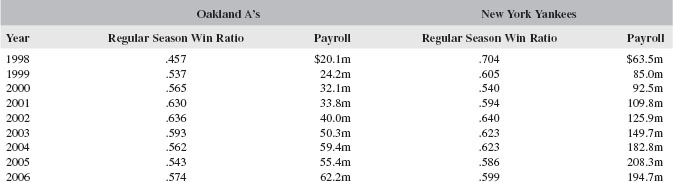
Source: International Journal of Sport Finance. Used with permission from Fitness Information Technology.
Two benchmarking analyses have been developed for the relationship between win ratios and payroll costs for all of the MLB teams over the nine-year period, 1998–2006. The first benchmark analysis is a ratio analysis using average payroll costs per win. The cost-per-win ratio is the inverse of the output-input efficiency ratio with payroll costs as the input and games won as the output. There are two methodological issues involved in calculating the cost-per-win ratio for MLB teams. First, given that the data set includes nine years with substantial salary inflation, it is necessary to convert the nominal payroll costs into inflation-adjusted (i.e., real) payroll costs. In both benchmarking analyses payroll costs have been converted to 1998 MLB dollars using a conversion factor calculated as the total MLB payroll costs in the specified year divided by the total MLB payroll costs in 1998. This provides a measure of the cumulative salary inflation between 1998 and the specified year. Dividing all team payroll costs in the specified year by the conversion factors converts the team’s payroll costs into 1998 MLB dollars. The second methodological problem with the cost-per-win ratio is the choice of an appropriate baseline from which to calculate the (marginal) cost-per-win ratio. Exploratory data analysis (both graphical and simple regression analysis) indicates that in terms of 1998 MLB dollars the appropriate pay-performance baseline is $8.75 million payroll costs and 50 wins.
Table 6 lists the average cost-per-win for all MLB teams over the period 1998–2006 calculated in 1998 MLB dollars using the baseline of 50 wins and $8.75 million payroll costs. It can be seen that the MLB average is $1.02 million dollars for each win over 50. Oakland ranked first as the most efficient MLB team over the period with a cost-per-win ratio of $414,647 representing an efficiency gain of 59.3% relative to the MLB average. The second most efficient team is the Minnesota Twins with a cost-per-win ratio of $470,990 (implying an efficiency gain of 53.8%). The other highest ranking teams are the Florida Marlins ($514,884 per win), Montreal Expos ($556,674 per win), and Pittsburgh Pirates ($716,905). (It should be noted that the cost-per-win ratio for the Expos is based only on seven seasons since the franchise has been replaced by the Washington Nationals from season 2005 onwards.)
The three most inefficient teams over the period have been Baltimore ($1,680,911 per win) and the two New York teams, the Yankees ($1,535,662 per win) and the Mets ($1,432,323 per win). Baltimore’s cost-per-win ratio is 64.9% above the MLB average. The Yankees show an efficiency loss of 50.7%. Hence, it is clear that the Moneyball effect has been considerable whether you compare Oakland with the extreme of the Yankees or the MLB average. A 59% efficiency gain over a nine-year period indicates a truly remarkable sustained competitive advantage in a highly competitive industry with competition at the core of the production process not just limited to the market process.
….
The … differences in payroll costs between MLB teams explain just less than one quarter of the variation in win ratios between teams and between seasons. Inclusion of the persistence effects of performance in the previous season increases the explanatory power to around 37%. Although payroll costs are clearly an important explanation of why some MLB teams win more regular-season games than other teams, financial differences are not overwhelmingly dominant in determining win–loss records. The MLB is not a league that exhibits a high degree of financial determinism compared with, for example, the leading professional soccer leagues in Europe in which the static pay-performance relationship accounts for two-thirds or more of the differences in sporting performance of teams….
The structural … analysis again highlights the exceptional achievement of Oakland as an organization. It is estimated that over a nine-year period Oakland won 144 games more than would have been predicted by a simple win-payroll benchmark model…. Sporting competition tends to create a reversion-to-mean process in which teams tend to gravitate towards a long-term equilibrium determined by the market fundamentals (i.e., the financial size of a team’s local market). To deny the sporting equivalent of the law of gravity for nine seasons is indeed remarkable. It should be noted that the Yankees emerge as a better-than-benchmark team with 18.2 wins more than predicted by their payroll costs. The Yankees are big spenders but the benchmark analysis suggests that the team spends its money effectively so that it is a high-budget, high-achievement organization. In contrast, Baltimore is a high-budget, low-achievement team with the sixth highest average payroll expenditure over the period but an average win ratio of .449. Baltimore is estimated to have lost 96.4 games more than would be expected by an average efficiency team with the same level of payroll costs. Only Tampa Bay has shown greater inefficiency than Baltimore with 96.6 games below benchmark.

Source: International Journal of Sport Finance. Used with permission from Fitness Information Technology.
1. All payroll costs converted to MLB dollars to remove inflation effect. Conversion factors calculated by dividing total MLB payroll costs in specified year by total MLB payroll costs in 1998.
2. Average payroll costs per win calculated relative to baseline of 50 wins and $8.75m payroll costs (1998 MLB dollars).
OAKLAND A’S: EXPLAINING THE MONEYBALL EFFECT
Successful organizations with a sustainable competitive advantage over rival organizations can be viewed as having either resource-based or knowledge-based advantages (or a combination of both). The resource-based view (RBV) of the firm (Wernerfelt, 1984) focuses on qualitative resource-based advantages in industries characterized by resource heterogeneity. In such industries the firms with a sustainable competitive advantage are those that possess rare, unique strategic resources that are specific to the individual firm and difficult for rival firms to imitate and replicate. By contrast, in industries in which there is a high degree of resource homogeneity in the sense that the higher-quality strategic resources that yield a competitive advantage are more mobile between firms and potentially tradable on a market, the more successful firms tend to have a quantitative resource-based advantage, and are able to utilize their greater economic power to purchase the higher-quality strategic resources. In order to compete effectively with resource-rich firms, resource-poor firms need to develop a “David” strategy in which they create knowledge-based advantages. Using a distinction originally proposed by Makadok (2001), there are two types of knowledge-based advantages—resource-picking advantages and capability-building advantages. Resource-poor organizations can compete effectively if they are better at selecting resources and/or deploying resources. A successful resource-picking “David” strategy involves developing mechanisms that allow the organization to be more effective in identifying higher-quality resources at lower per unit cost in competitive situations with signifi-cant uncertainty over the future performance of individual resources. A successful capability-building David strategy requires the organization to develop mechanisms for the utilization of individual resources that yields higher levels of future performance from resources than can be achieved by rival organizations.
In professional team sports, the economic power of teams is a product of history and geography. Teams located in large metropolitan areas and a history of sporting success have the largest fan bases and are, therefore, more able to compete for the best playing talent. It is the concern with maintaining competitive balance to ensure the continuing interest of fans and financial viability of the league that has led professional sports leagues to introduce various product-market and labor-market restrictions to limit the ability of big-market teams to corner the market for the best players (Quirk & Fort, 1992). Professional sports leagues have tried to equalize team revenues through cross-subsidization mechanisms such as sharing gate receipts and collective selling of media and other image rights. Alternatively, leagues have regulated the players’ labor market via salary caps, luxury taxes on excessive payrolls, reserve clauses, transfer fees, and centralized drafting of new players.
The MLB has been one of the least regulated professional sports leagues…. [T]here has been a three- or four-fold difference in payrolls between the big-market goliaths in the MLB such as the New York Yankees and the smaller-market teams such as the Oakland A’s. The core of the knowledge-based “David” strategy developed by Billy Beane has been the systematic use of player performance data in player recruitment, player valuation, and team field tactics. Beane recognized the value of the insights provided by sabermetrics, the statistical analysis of baseball, particularly the work of Bill James. James is the guru of sabermetrics who had started to publish his statistical analysis of baseball in his Baseball Abstract annually in the 1980s but had remained largely ignored by MLB teams (Gray, 2006). Moneyball tells the story of how Beane has used the insights of sabermetrics to develop resource-picking and capability-building advantages.
Much of Moneyball deals on the resource-picking strategies of Oakland, particularly in the player draft. Beane shifted the team’s recruitment strategy away from high school graduates towards college players with exceptional playing records. There are three advantages of focusing more on college players as draft picks. First, college players are older with more playing experience at an elite level and, as a consequence, teams can have a better appreciation of whether or not players can cope with the demands of professional baseball. Second, the playing records of college players are much better recorded in much greater detail than high school playing records. College baseball statistics are also much more informative since the quality of the opposition is more uniform. Finally, since other teams are predominantly chasing after high-school draft picks and college players are often perceived as “rejects” who have previously failed to be drafted to the MLB, the market valuations of college players tend to be significantly lower. Hence there is a potential profitable trading opportunity to sign playing talent at a lower cost. Oakland’s focus on college players in the draft is one of the factors explaining their significant efficiency gains in the average cost per win….
Another key factor in the Oakland’s low cost per win has been the exploitation of the market inefficiency in the valuation of hitters. It is the proposition that the MLB players’ labor market has systematically undervalued the productive value of hitters that Hakes and Sauer (2006) refer to as “the Moneyball hypothesis”. Batting and slugging averages are the conventional baseball statistics for hitters but these statistics only measure hitting. Statistical analysis shows that on-base percentage (OBP), measuring the proportion of at-bats that the hitter reaches base either by hits or walks, is a better predictor of win ratios. Since MLB teams have focused on the conventional measures of hitter performance rather than OBP, this would imply that the market valuation of players would tend to undervalue players who rank much better on their OBP statistics than batting and slugging averages. This market inefficiency would, in turn, create a potential profitable trading opportunity that could allow teams using OBP to identify potential recruits and effectively buy runs more cheaply than rival teams.
Hakes and Sauer tested the Moneyball hypothesis…. Hakes and Sauer estimated a statistical model of team win-ratios in the MLB using data for seasons 1999–2003. They found that the best predictive model of MLB win-ratios included both OBP and the slugging average. These two hitter performance variables jointly explained 88.2% of the variation in regular-season win-ratios between teams over the five seasons. The estimated coefficient on OBP was found to be more than twice as large as that for the slugging average. Thus, the production (i.e., win contribution) value of OBP is significantly greater than the production value of the slugging average. Hakes and Sauer estimated a benchmark salary model for hitters for seasons 2000–2004. Their benchmark salary model included OBP, the slugging average and a set of control variables—plate appearances, arbitration eligibility, free-agent status, catcher, and infielder. Hakes and Sauer discovered that slugging average was a highly significant determinant of hitter salaries in each season between 2000 and 2003. In contrast, OBP was statistically insignificant every season over the same period and the magnitude of the estimated coefficient was much smaller (and, indeed, had a small negative effect in 2001). Thus, Hakes and Sauer found very strong evidence of market inefficiency with a significant discrepancy between the production value of OBP and the market (i.e., salary) value. It is this market inefficiency that Billy Beane exploited very effectively. Interestingly, Hakes and Sauer extended their benchmark salary model to 2004, the season after the publication of Moneyball. By 2004, OBP had become a highly significant determinant of hitter salaries in the MLB with an estimated coefficient larger than that for the slugging average. The market inefficiency had been corrected following the publication of Moneyball which, of course, begs the question as to why Oakland allowed the publication of a book that made public some of the sources of their competitive advantage. The lesson is clear: if you have a knowledge-based competitive advantage, keep it secret from your rivals as long as possible.
Moneyball also outlines that Oakland’s “David” strategy is not purely a resource-picking knowledge-based advantage in the identification and remuneration of new recruits. It is clear that the analysis of player performance data has led to capability-developing knowledge-based advantages in the deployment of players during games. The team’s field tactics are also influenced by the statistical analysis of what wins and loses games. For example, in line with the production value of OBP, Oakland stresses the importance of pitch selection for hitters. Team tactics also put much less importance on stealing bases compared to other teams. Oakland believes that statistical analysis shows stealing bases to be a high-risk, low-reward tactic.
BEYOND BASEBALL: FROM ATOMISTIC TO COMPLEX TEAM SPORTS
The Moneyball approach requires reliable performance data for individual players in order for teams to be able to evaluate formally using, for example, statistical analysis to quantify what each player has contributed to the overall team performance. However, player performance is only highly separable in atomistic striking and fielding team sports such as baseball and cricket. It is no surprise that the academic research on the economic value of elite athletes in professional team sports has been concentrated in the MLB beginning with the estimation of the marginal revenue product (MRP) of hitters and pitchers by Scully (1974). Not only is there extensive publicly available data on individual player salaries in the MLB (e.g., the USA Today website) but there is also a strong statistical relationship between performance statistics for hitting and pitching, and the team’s win-loss record. For example, in his 1974 study Scully found that around 88% of the team win percentage could be explained by the team slugging average and the team strikeout-to-walk ratio after controlling for league affiliation and divisional standing. Decomposing the aggregate team hitting and pitching statistics into individual player components allowed Scully to estimate the win-equivalent contribution of each hitter and pitcher, which he then translated into a financial valuation using the estimated relationship between team revenues and team wins.
Replicating Moneyball and Scully’s pay-and-performance analysis in invasion team sports such as the various codes of football, field and ice hockey, and basketball is much more problematic. Invasion team sports are much more complex and hence the separability of individual player contributions is considerably more difficult. Invasion team sports involve a group of players co-operating to move an object (e.g., a ball or puck) to a particular location defended by opponents (e.g., across a line or between goalposts). There are several dimensions of complexity in invasion team sports. First, the range of player actions is much greater and includes tackling to regain possession, moving the ball forward via passing, receiving, running and/or dribbling, and attempting to score by shooting or crossing the line. Second, player actions are highly independent. Scoring requires the ball to be moved forward which, in turn, requires the team to have regained possession. Defensive and offensive plays are interdependent. Third, many player actions are joint actions. For example, more than one player may join together to tackle an opponent in possession in some codes of football. Fourth, invasion games vary in the degree to which there is continuity or segmentation between offensive and defensive plays. Association football (i.e., soccer) is the most complex in this respect with a continuous flow, whereas American football is highly segmented with play stopped and players interchanged after turnovers in possession. Finally, linked to the degree of continuity in play, invasion games vary in the extent to which playing roles are specialized. Again soccer is the most complex in this respect with all outfield players required to be highly competent both defensively and offensively. In contrast, American football has highly specialized defensive, offensive, and kicking units.
There are three measurement problems that must be resolved in order to undertake detailed player performance analysis in complex invasion team sports—the tracking problem, the attribution problem, and the weighting problem. The tracking problem refers to the identification, categorization, and enumeration of different types of player actions in and out of possession and including spatial coordinates of where the actions have taken place on the field of play. The attribution problem is the problem of how to allocate the individual contributions to joint and interdependent actions. The weighting problem is that concerned with determining the significance of each individual action to the overall match outcome.
The tracking problem is largely an issue of technology. Historically, performance statistics in complex team sports were limited to appearances, scoring, and discipline. Statistics on players’ actions were recorded during matches by coaches and other observers using basic “paper-and-pencil” notational analysis. The advent of TV video playback at the elite level allowed coaches to develop much more sophisticated systems of notational analysis for private use by teams but the time-demands limited how much information was extracted. The tracking problem has been largely solved in recent years by two IT developments: (i) software for automated video analysis of matches and (ii) in-stadium sensors and image recognition software to allow the direct tracking of players. For example, in several leading professional soccer leagues, many of the top teams now use player tracking systems developed by the French company, Sport-Universal Process, or the UK-based company, ProZone. These systems provide data on player actions in possession and spatial movements including speed and distance covered by players. These tracking systems allow “bird’s-eye” animated reconstructions of games to facilitate the analysis of individual player decisions as well as team shape and spatial coordination in and out of possession. The next stage in the development of tracking systems will be the provision of real-time feed including the use of some form of chip technology to transmit location and physiological data directly from players.
With the tracking problem solved by technology and the attribution problem amenable to agreed decision rules and conventions for the allocation of individual contributions to joint/interdependent actions, the principal measurement issue that remains is the weighting problem of how to determine the relative importance of different player actions toward overall match outcomes. There are two general types of solution to the weighting problem—a subjective, judgment-based approach or a more “objective” statistical approach. The subjective judgment-based approach involves an expert developing a weighting system based on their own experience and judgment. This is the approach adopted by, for example, the Opta Index in English soccer which provides player ratings based on a composite of player actions using a weighting system developed by Don Howe, the former Arsenal and England coach.
The statistical approach involves the determination of an appropriate set of weightings by estimating the degree of statistical association between match outcomes and the number of different types of player actions using a sample of games. One particular statistical method is multiple regression analysis, which involves specifying and estimating a linear relationship between outcomes and the frequency of different actions. However, the problem with the statistical approach in invasion team sports is the hierarchical nature of the game with the higher-level actions, scores, and saves (i.e., the blocking of scoring attempts by opponents) dependent on lower-level actions to create scoring opportunities and limit opposition scoring opportunities. Figure 1 provides a graphical illustration of the hierarchical structure of a complex invasion game. Higher-level actions are causally closer to final match outcomes and, as a consequence, are likely to be the best statistical predictors of outcomes with the highest weightings. Hence, players who specialize more in higher-level actions will tend to receive a disproportionately high estimated win contribution compared to players specializing in more lower-level actions if a purely statistical approach is adopted with no recognition of the dependency of higher-level actions on lower-level actions.
The statistical approach toward the weighting of player actions necessarily requires expert judgment to determine the relative weightings between different levels in the structural hierarchy, with statistical estimation used to determine the relative intra-level weightings between actions at the same level. Expert judgment may also be needed to adjust the estimated statistical weightings of those player actions that act as a good statistical predictor of opposing player actions. For example, a high observed frequency of positive defensive actions that prevent scoring opportunities for the opposing team can statistically be a good proxy for the amount of offensive activity by opponents leading to a negative weighting reflecting that the more opponents attack the more likely a team is to lose.
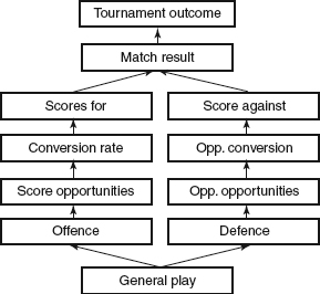
Figure 1 A Hierarchical Structural Model for Invasion Team Sports
Source: International Journal of Sport Finance. Used with permission from Fitness Information Technology.
The hierarchical structural model of a complex invasion game illustrated in Figure 1 can be used to provide a framework for analyzing the drivers of match outcomes. The contributions of different types of general play to creating scoring opportunities and limiting opposition scoring opportunities can be estimated statistically. The win contribution of general play can be determined using the average league conversion of scoring opportunities. This provides a benchmark to determine the extent to which a team has deviated from the average league performance because of differences in player effectiveness with respect to identifiable individual contributions in the form of different types of general play, scoring conversion rates and save rates in games with a designated goalkeeper/goalminder. The residual component can be categorized as team effectiveness referring to deviations from the average league benchmark that cannot be predicted on the basis of individual player contributions. Offensive team effectiveness can be measured as the difference between the actual frequency of scoring opportunities created and the predicted frequency given the observed own-team general play. Similarly, defensive team effectiveness can be measured as the difference between the actual frequency of opposition scoring opportunities and the predicted frequency given the observed own-team general play. An application of this performance analysis and benchmarking in English Premiership soccer is discussed in the next section.
APPLICATION: ANALYZING TEAM PERFORMANCE IN ENGLISH PREMIERSHIP SOCCER
The complexities of analyzing player performance in a complex invasion team sport are best appreciated by examining an actual application. Detailed player performance data is often confidential and provided to teams on a commercial basis, and hence is usually either unavailable or prohibitively expensive for academic researchers. However, the Opta Index (1999, 2000, 2001, 2002) has published detailed soccer player performance data in the Football Yearbook covering four seasons—1998–99 through 2001–02 of the FA Premier League (FAPL) in England. The Yearbook contains season-total data for 25 player statistics for every outfield player including passing, crossing, dribbling, defending, and goal attempts. In addition there are 14 player statistics for goalkeepers including the save-shot ratio. With 20 teams competing in the FAPL annually, it is possible to construct a team dataset with 80 team-season observations for each variable.
A hierarchical structural model based on the framework shown in Figure 1 was estimated using multiple regression analysis.
….
A bottom-up hierarchical analysis of deviations from benchmark was conducted in which the League Points value of lower-level actions is determined by assuming average-league performance at higher levels. This allows the team’s deviation from average-league performance (51.887 points) to be decomposed. Six types of deviation from benchmark are identified:
(i) General Play: deviation due to difference between team and average-league frequency of different types of general play
(ii) Striking: deviation due to difference between team and average-league conversion rates
(iii) Goalkeeper: deviation due to difference between team and average-league save-shot ratio
(iv) Offence: deviation due to difference between actual frequency of own shots at goal and predicted number given own general play
(v) Defense: deviation due to difference between actual frequency of opposition shots on goal and predicted number given own general play
(vi) Result: deviation due to difference between actual League Points and predicted League Points given actual number of goals scored and conceded
The first three categories are defined as (individual) player effectiveness since the deviations can be clearly attributed to individual players. Categories (iv)–(vi) are defined as team effectiveness since the deviations can only be attributed to the team as a whole and not to any specific player.
An illustration of the hierarchical analysis of deviations from benchmark is provided in Figure 2 for Arsenal in season 2001–02. Arsenal finished as Premiership champions with 87 points, which represents a benchmark deviation of 35.11 points (relative to the league average over the four sample seasons). This benchmark deviation is fairly evenly allocated between player effectiveness and team effectiveness. It is estimated that if goal conversion rates for both Arsenal and their opponents are set equal to the league average, then the greater frequency of general play actions (e.g., passing, dribbling, crossing, and defending) by Arsenal’s outfield players relative to the Premiership average contributed 12.86 points (i.e., 36.63%) of the total benchmark deviation. Arsenal’s better than average shot conversion rate contributed another 9.38 points above the league average. The only category in which Arsenal had a negative deviation was goalkeeping. Arsenal’s save-shot ratio was lower than the league average due to their first-choice goalkeeper being injured for a significant part of the season with no adequate backup replacement. Arsenal’s team effectiveness shows that their outfield players jointly created more shooting opportunities and allowed fewer opposition scoring opportunities than would have been predicted by the general play of their individual players. However, most of the team effectiveness is due to results deviation with Arsenal gaining 11.42 points more than would have been predicted given the total goals scored and conceded. This fits with the general perception of Arsenal as a team that is defensively strong and maximizes its return from goals scored. (Indeed Arsenal fans have long used the chant “one-nil to the Arsenal” to intimidate the opposition with the belief that once their team had scored, the defense would ensure that the lead was protected.) …
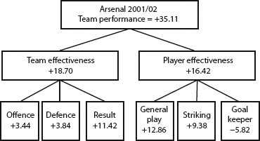
Figure 2 Benchmark Analysis, Arsenal, FA Premier League, 2001–02
Source: International Journal of Sport Finance. Used with permission from Fitness Information Technology.
The two dominant teams over the four seasons were Manchester United and Arsenal. Manchester United won the Premiership in seasons 1998–99, 1999–00, and 2000–01 and finished third in season 2001–02. Arsenal won the Premiership in season 2001–02 and finished runners-up to Manchester United in the other three seasons…. [T]here is a very different distribution between the two teams as regards the extent to which their deviation from the average-league benchmark is due to player effectiveness or team effectiveness. In the case of Arsenal, the team averaged 77 points (benchmark deviation = 25.11 points) over the four seasons with a relative equal balance between player effectiveness and team effectiveness. By contrast Manchester United’s average-league deviation of 29.86 points is almost entirely due to player effectiveness. Indeed over the four seasons it is estimated that team effectiveness cumulatively contributed only around 0.5 league points out of total benchmark deviation of 119.5 points.
This benchmark analysis suggests that the two teams adopted very different strategies towards achieving a sustainable competitive advantage. Using the distinction proposed by Makadok (2001), Manchester United could be considered as adopting a resource-picking strategy whereas Arsenal developed more of a capability-building strategy. Financially, Manchester United is one the biggest soccer teams in the world and over the sample period outspent Arsenal on wages by a margin of around 25%. There is a high statistical correlation of 0.801 between total wage costs and player effectiveness across all teams over the four seasons whereas the corresponding correlation between total wage costs and team effectiveness is only 0.195. In other words, player effectiveness can be acquired. Manchester United has had the necessary financial resources available and has been successful in its ability to identify and recruit highly effective players. Arsenal, on the other hand, has had more limited financial resources although still significantly more than the average Premiership team. As well as acquiring above-average player effectiveness, Arsenal has been able to develop the highest level of team effectiveness in the FAPL in the four sample seasons. Hence it could be considered that Arsenal, at least in terms of achieved results, has emulated the Oakland A’s in the sense of bridging the gap with a resource-richer rival by developing more knowledge-based David strategy. Unlike Oakland, however, the details of that knowledge-based advantage have not been made public. What is known is that the Arsenal head coach, Arsene Wenger, is an economics graduate who makes extensive use of player tracking data and has a reputation for spotting and developing young players.
CONCLUSION
The Moneyball message from the achievements of the Oakland A’s under the leadership of Billy Beane is that there is significant value to be derived from systematic (i.e., statistical) analysis of player performance. Oakland has achieved a sustained competitive advantage over an eight-year period to date by using statistical analysis to inform their decisions on recruitment, remuneration, and field tactics. Sabermetrics has become a key input into the knowledge-based “David” strategy that has allowed the low-budget A’s to compete effectively with the big-market goliaths such as the New York Yankees. The strategic resource in Oakland’s success has not been the player performance data which is a commodity available to all MLB teams. The strategic resource has been the ability of the Oakland management under the leadership of Billy Beane to create valuable private information through the analysis, interpretation, and application of the data.
There are three barriers to the transferability of the Moneyball approach to other team sports—the technological barrier, the conceptual barrier, and the cultural barrier. The technological and conceptual barriers are created by the complexity of invasion team sports. Teams need the technological capability to be available to track individual player actions and movements. Teams also need the conceptual framework to analyze player performance in the context of highly interdependent team play in which individual player actions are not separable. The technological barrier has been largely overcome through the development of video analysis and tracking systems. The conceptual barrier is more difficult but, as the analysis of Premiership soccer in this study has illustrated, it is possible to develop hierarchical structural models that can provide a conceptual framework to analyze and evaluate the contributions of individual players in complex invasion team sports.
The most enduring barrier towards the transferability of the Moneyball approach is the cultural barrier. Moneyball is a very different mindset in which statistical analysis is integrated into expert judgment-based decision-making systems. It is a different way of doing things that inevitably is dismissed as useless and inappropriate by those wedded to existing methods. Indeed much of the Moneyball story is about the clash of cultures between those committed to more subjective methods of analysis such as the scouts and those led by Billy Beane who relied more heavily of statistical analysis of performance data. It is a classic case of the “shirts” and the “suits”. The shirts are those who are experienced in the specifics of the production process. In the case of professional team sports, the shirts are ex-players. The suits are those with more general management experience. Moneyball is the story of the suits invading the domain of the shirts and the tensions and conflict generated between two different mindsets. The cultural barrier is the most difficult to overcome. A successful champion of the new approach is crucial. Michael Lewis’s best-selling book, Moneyball, has helped to establish Billy Beane as the successful champion of player performance analysis in sports around the world. But, of course, it is important to differentiate between bestseller hype and management reality. The book focuses on the science of player performance analysis but, as the subtitle of the book highlights, the application is an art. Billy Beane is a “shirt-suit,” an ex-MLB player who is a talented talent-spotter and player trader using both expert judgment and data analysis. After all, player performance analysis can only ever make a team competitive by calculating systematically the expected returns from alternative options in player recruitment and remuneration and field tactics. Winning also requires taking risks and that can never be a matter of pure calculation. Knowing which risks to take always involves judgment. Ultimately the main lesson of Moneyball is transferable to other sports and also to non-sporting organizations. Organizational effectiveness is both an art and a science; ignoring one in favor of the other is likely to diminish rather than enhance the organization’s effectiveness. Successful performance management requires both “hard” data analysis and “soft” expert judgment.
References
….
Gray, S. (2006). The mind of Bill James: How a complete outsider changed baseball. New York, NY: Doubleday.
Hakes, J. K., & Sauer, R. D. (2006). An economic evaluation of the Moneyball hypothesis. Journal of Economic Perspectives, 20, 173–185.
Lewis, M. (2003). Moneyball: The art of winning an unfair game. New York, NY: Norton.
Makadok, R. (2001). Toward a synthesis of the resource-based and dynamic-capability views of rent creation. Strategic Management Journal, 22, 387–401.
Opta Index (1999, 2000, 2001, 2002). Football yearbook (various editions). London: Carlton Books.
Quirk, J., & Fort, R. D. (1992). Pay dirt: The business of professional team sports. Princeton, NJ: Princeton University Press.
Runciman, D. (2007). Can this American coach and this book deliver success in English football? The Observer Sport Monthly, 84, 20–29.
Scully, G. W. (1974). Pay and performance in Major League Baseball. American Economic Review, 64, 915–930.
Wernerfelt, B. (1984). A resource-based view of the firm. Strategic Management Journal, 5, 171–180.