13

Using Sensors with Processing and Arduino

You’ve explored keyboard, mouse, and webcam inputs in Processing, and built a custom game controller with a Makey Makey. But what if you want to create something that responds to less-conventional inputs? With a little help from an Arduino, you can Monitor temperature, ambient light, and more with Processing.

This chapter focuses on using Processing’s Serial communication library to bring data from the world around you into your sketches. The Serial protocol sends data 1 bit at a time, allowing devices to communicate simply and efficiently.

In this chapter, you’ll read sensor values for temperature, sound, and light with an Arduino and visualize those values in Processing. In “Taking It Further” on page 261, I’ll also walk you through sending data to the microcontroller from Processing to control the color of a red/green/blue (RGB) LED.

GATHER YOUR MATERIALS

In this project, you’ll need the following materials:

• One mini USB cable (CAB-11301)

• One SparkFun Digital Sandbox (DEV-12651)

WHAT IS A MICROCONTROLLER?

A microcontroller (like the one in Figure 13-1) is similar to the central processing unit (CPU) on your computer, but it operates much slower and can do only one process at a time. A microcontroller can run code, but unlike your multitasking CPU, it just runs a single program over and over until you reprogram it.

Microcontrollers control many of the electronics in your car, your kitchen, and even your alarm clock. You can program these chips to read temperatures, turn motors and lights on and off, and even communicate with other devices! These controllers are in a number of maker projects, from automated lawnmowers and DIY drones to cube satellites and interactive art installations.

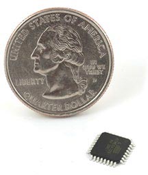
FIGURE 13-1: An ATMEGA328 microcontroller

Microcontrollers have pins (tiny metal legs) that you can use to read data from sensors and transmit data to control hardware. But without a circuit, a microcontroller is just a bit of plastic and metal. To have Processing communicate with a microcontroller, we’ll use a development platform called Arduino.

WHAT IS ARDUINO?

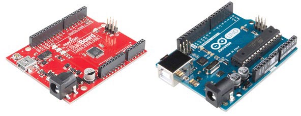
Arduino is an electronics platform that uses Atmel microcontrollers to make hardware and software easy to use together. Arduino, like Processing, is open source, so there have been a number of copies, mashups, and other boards based on the platform. For example, the RedBoard in Figure 13-2 is SparkFun’s major Arduino-compatible board.

FIGURE 13-2: The SparkFun RedBoard (left) and an Arduino Uno (right)

This chapter will scratch the surface of Arduino and show you how to use it with Processing. My goal is to give you just enough knowledge to make you dangerous. That means there will be some hand waving. If you want more detailed tutorials, I recommend SparkFun’s Digital Sandbox tutorial (https://learn.sparkfun.com/tutorials/digital-sandbox-arduino-companion/) and the SparkFun Inventor’s Kit experiment guide (https://learn.sparkfun.com/tutorials/sik-experiment-guide-for-arduino---v32).

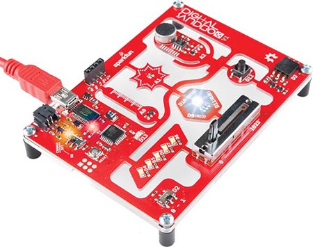
THE SPARKFUN DIGITAL SANDBOX

In addition to the RedBoard, SparkFun also develops other boards that you can program with Arduino software, like the Digital Sandbox in Figure 13-3.

FIGURE 13-3: Digital Sandbox input and output guide

USB Mini-B Connector: Used to connect to a computer.

JST Right-Angle Connector:Used to supply power to the board.

Slide Switch for Charging: Used to charge a lithium polymer battery that is plugged in to the two-pin JST connector, while the Digital Sandbox is connected to a computer and the slide switch is in the ‚on‛ position.

Reset Button: This is a way to manually reset your Digital Sandbox, which will restart your code from the beginning.

Slide Switch (Pin 2): “On” or “off” slide switch.

LEDs (Pins 4-8):Use one or all of the LEDs (lightemitting diodes) to light up your project!

LED (Pin 13): Incorporate this into your sketch to show whether your program is running properly.

Temperature Sensor (Pin A0):Measures ambient temperature.

Light Sensor (Pin A1): Measures the amount of light hitting the sensor.

RGB LED (Pins 9-11); RGB (red/green/blue) LEDs have three different color-emitting diodes that can be combined to create many colors.

Slide Potentiometer (Pin A3): Change the values by sliding it back and forth.

Microphone (Pin A2): Measures how loud something is.

Push Button (Pin 12): A button is a digital input. It can be either “on” or “off.”

Add-on Header (Pin 3): Three-pin header for add-ons. Example add-ons are servos, motors, and buzzers.

The Digital Sandbox is an Arduino with a bunch of inputs and outputs built into the board, so you can focus on programming over building circuits. In essence, the Digital Sandbox is designed to be a training board for Arduino, so the labels A0 through A3 and D2 through D13 on the Digital Sandbox correspond to pin names you’d see on a standard Arduino. These labels also correspond to the pin names in the Arduino programming language.

NOTE

If you own an Arduino and the parts to build the circuits for this chapter, you could use those instead of buying a Digital Sandbox. You’ll find a wiring diagram for a standard Arduino and breadboard in the DigitalSandbox_on_bb.jpg file of the online resources at https://nostarch.com/sparkfunprocessing/. The programming is all the same as what I describe in this project.

For simplicity, and to keep you focused on Processing, we’ll use the Digital Sandbox to build this chapter’s project. I recommend using the Digital Sandbox in future Processing-to-Arduino explorations, too, as it allows you to get up and going quickly without spending a lot of time wiring.

INSTALLING THE ARDUINO SOFTWARE

Like Processing, Arduino’s integrated development environment (IDE) is free to download. You’ll use that software to program the hardware. Go to https://arduino.cc/download/ and download the latest stable version of the Arduino IDE for your operating system. If you get stuck at any point, check out the “Installation Resources” on page 240 and read the official Arduino installation guide for your system for more detailed instructions.

Installing Arduino and Drivers on Windows

If you’re running Windows, download the Windows installer package, which should include the required drivers for Arduino and prompt you to install them.

Once it’s downloaded, open the installer executable. You will be greeted with a pretty standard license agreement. Select Agree (assuming you do), and a dialog will appear with installation options, as shown in Figure 13-4.

FIGURE 13-4: Arduino installation options

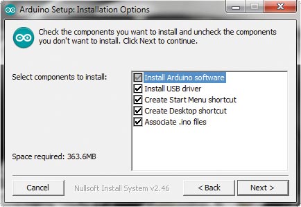
Select the options Install Arduino software and Install USB driver. The others are up to you, though I do suggest selecting the Associate .ino files box for ease of opening files later.

Once you make your selections, click Next. The installer will ask where you’d like to install it; you can leave this at its default. Click Next to begin the install process.

Once the install finishes, click Complete. Select that Arduino is trusted, and install the drivers. With that, your Windows machine should be ready to go with Arduino and the drivers installed.

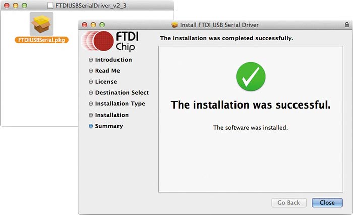
Installing Arduino and FTDI Drivers on OS X

If you’re an Apple user, download the OS X installer package from the Arduino website. When you open the downloaded folder, the Arduino app should be the only file it contains. Drag the app to your Applications folder to install Arduino. After that, there’s just one more step: downloading Future Technology Devices International (FTDI) drivers for the Digital Sandbox and any other Arduino that uses FTDI.

NOTE

FTDI chips translate the USB communication protocol to serial, and vice versa.

Go to FTDI’s drivers page at http://www.ftdichip.com/Drivers/VCP.htm (make sure you include the “chip” portion of the URL or you’ll end up buying flowers!) and find the correct download for your OS X system. Depending on your system, click the OS X link for 32-bit, 64-bit, or PPC (Power PC) to download the .dmg file.

Double-click the .dmg file, and you’ll see a single install package called FTDIUSBSerial.pkg. The directory will look like Figure 13-5. Double-click that option to start the driver installation process. Accept the license agreement and click Continue to finish.

FIGURE 13-5: FTDI installation on Mac OS X

Installing Arduino on Ubuntu Linux

There are too many Linux distributions to cover all of them here, but I’ll walk you through the basic install on Ubuntu 14.04. To install Arduino, navigate to the download page of the http://www.arduino.cc/ site and download the appropriate version; for most modern Ubuntu systems, you’ll probably want the Linux 64-bit version. Then, navigate to your downloads directory (or wherever you might have saved the file), right-click the compressed package shown in Figure 13-6, and select Extract Here.

FIGURE 13-6: Arduino IDE download package

Once you’ve extracted the package, double-click the Arduino icon to run it. Alternatively, you can download a stable version of Arduino through your package manager interface or through the command line. If you are new to Linux, I highly recommend using the package manager and installing Arduino through the GUI.

NOTE

You may also need to add your user to the dialout group before you can actually upload code to the Arduino via USB. If this is the case, you should see a message to that effect when you run the IDE for the first time.

You’ll also have to install Java and a few other dependencies for Arduino to work properly on Linux. From a command line, enter the following command to install Java and avr-gcc, which is the compiler used for Linux.

After everything downloads, you’ll be asked for permission to install it all. Press Y to agree to the installation. Once Arduino is installed, you can run it from the command line by navigating to its directory and running the Arduino script as follows:

Or to enable a double-click option so you can to run Arduino from the desktop GUI, double-click on the file from your GUI file manager, and select Edit Preference from the drop-down menu. In the dialog that appears, select Double Click to Open and Ask Each Time from the options. Now, double-click the script file and select Run from the pop-up window. The Arduino IDE should launch. If it doesn’t, or you’re not running Ubuntu, try visiting the Linux link in the “Installation Resources” box for more detailed instructions from the Arduino website.

INTRODUCING THE ARDUINO IDE

Plug your Digital Sandbox into your computer. If you see a notification that your device is being installed, don’t fret: your computer is just making sure the correct drivers are installed.

Two LEDs (light emitting diodes) on the Digital Sandbox should be turned on. The power LED should always be on if the board is powered, so it should glow steadily. The LED labeled D13 should be blinking because SparkFun preprogrammed the microcontroller with a simple Arduino program (also called a sketch) to test the board. So that blinking LED means you are good to go so far!

Open the Arduino software, and after a splash screen, you will see the IDE in Figure 13-7.

FIGURE 13-7: The Arduino IDE

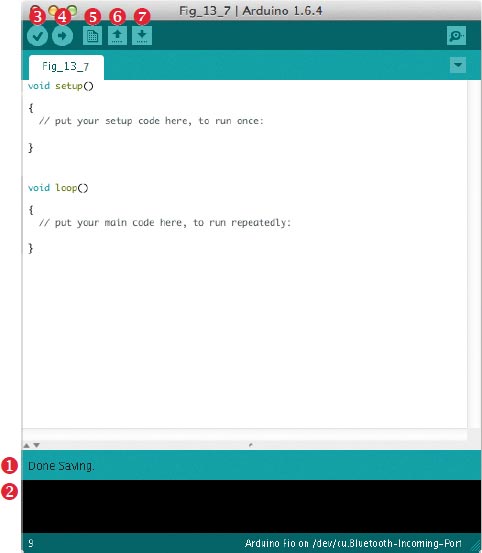
The Arduino IDE should look familiar because it’s based on Processing, but there are a few differences. The code window and console function similarly to their Processing counterparts. If your sketch has errors, they will pop up in the alert bar ❶ and console ❷. At the top are the Verify ❸ and Upload ❹ buttons (the check mark and right arrow, respectively).

Since Arduino code runs on the Arduino board, you have to upload it to the Sandbox for it to run, so the IDE doesn’t offer the same immediate feedback as Processing’s Run button. You can, however, verify your sketch, which checks to make sure there are no errors in your code without uploading it to the board.

Continuing right from the Verify and Upload buttons, you should also see the New ❺ button for opening a new sketch, Open ❻ for opening an existing sketch, and Save ❼ for saving your current work.

SELECTING YOUR BOARD AND CHOOSING A PORT

NOTE

To figure out if your board is on a particular serial port, unplug it and refresh your list of ports. If the updated list has one unselectable option or a port has disappeared, that is the port for your board.

Since there are so many different Arduino boards, you need to tell the Arduino IDE which one is plugged into your computer. First, click Tools Board to view a list of board types. The Digital Sandbox works like an Arduino Fio board, so select Fio from the list.

Next, select Tools Port . . . to specify which communication port the board is on. In Windows, you should see a COMX option, where X is a port number. If you have multiple COM port options, the Sandbox COM port is usually the highest number in the list. Regardless of your operating system, select your port by clicking on it; when properly selected, the port will have a checkmark or dot next to it in the list, as shown in Figure 13-8.

FIGURE 13-8: Mac serial port selection

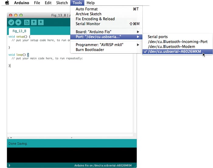
If you are running OS X, your serial ports list will look similar to Figure 13-8, instead of listing COM ports. If the FTDI drivers were installed correctly, you will have an option that reads /dev/tty .usbserial-<XXXXX>. You can ignore the others in the list; they’re your computer’s Bluetooth connection and other ports. Linux users will see a similar naming convention for the serial ports on their machines (for example, /dev/ttyUSB0), since Mac and Linux are both based on Unix and have similar directory structures for things like their serial ports.

With your board and serial port selected, you’re ready to code!

AN ARDUINO HELLO WORLD

In this section, you’ll program the Digital Sandbox with an Arduino sketch to make sure everything works correctly. Blinking an LED is the hardware version of Hello World, so we’ll start there.

Exploring an Arduino Sketch

First, let’s explore the basic structure of an Arduino sketch in Listing 13-1.

LISTING 13-1: The bare-bones Arduino sketch

This is the skeleton sketch you see when you open the Arduino IDE. It looks just like a basic Processing sketch, except that instead of draw(), there’s a loop() function that works exactly like draw(). You will also notice that in Arduino sketches, the keyword coloring is a little different from Processing, with most key words being a redorange color—but no need to worry about that too much.

Writing the setup() Function

The setup() code for blinking an LED is pretty simple. Open a new Arduino code window now and fill in the setup() function as follows:

First, specify which pin you want to control on the microcontroller and how you are going to use it with the pinMode() function ❶. This function takes two parameters as arguments: a pin number, which can range from 0 to 13, and a constant, which should be INPUT or OUTPUT. Passing INPUT tells the Arduino to set up a pin to receive data, and passing OUTPUT tells the Arduino that the pin will send data. Here, you tell the Arduino to set pin 4 as an output, because that pin is connected to the LED you want to blink on the Sandbox (in this case, D4). Any time you want to use a pin, you need to have a pinMode() function for it.

That’s all for the setup!

Writing the loop() Function

Now, you’ll tackle the loop() function, which is where you’ll actually blink your LED. As the second comment in Listing 13-1 states, the Arduino runs this code over and over again, at a speed of millions of lines of code per second. Conceptually, the loop() function for blinking an LED would work something like Figure 13-9.

FIGURE 13-9: How blinking works behind the scenes

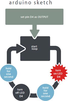
You only have to tell the Arduino to blink once inside the loop() function because when it reaches the end, the loop starts over again. Because the loop runs so fast, you also need to tell the microcontroller to wait or delay for a given amount of time, so you can actually see the LED blink.

In the same Arduino code window where you added the setup() function, write the loop() code shown in Listing 13-2 to translate the flow chart into the Arduino language.

LISTING 13-2: The loop() code for your blinking Arduino sketch

NOTE

TX is short for transmit, and RX is short for receive, and these LEDs light up any time data is passed between the board and the computer. Here, the sketch you just uploaded went from the computer to the Digital Sandbox.

The digitalWrite() function ❶ is like a code light switch; it allows you to turn pins on and off. You pass it two parameters: the pin number (0-13, corresponding to D0-D13 on the Arduino) and either HIGH (on) or LOW (off). Here, you turn pin 4 on.

Next, you wait for 1 second using the delay() function ❷, turn pin 4 off ❸, and wait for 1 second again ❹. From there, the sketch loops back up to the top.

Make sure your Digital Sandbox is plugged in to the computer, and click the Upload button. The two LEDs labeled TX and RX should blink really fast.

After TX and RX stop blinking, D4 should blink once per second, as shown in Figure 13-10.

FIGURE 13-10: Our best print rendition of D4 blinking

Congratulations on your first Arduino sketch! Before you move on, play around with this sketch a bit. Try replacing pin 4 with other output pin numbers, according to the labels in Figure 13-3 (you’ll need to change them in the pinMode() and digitalWrite() functions), and tweak the delay time for faster or slower blinks.

ANALOG VERSUS DIGITAL

Now that you know how to program an Arduino, let’s explore the two types of data you can use with the platform. Digital data has only two possible values: on and off, which correspond to 0 and 1 or HIGH and LOW, respectively, in a sketch. The power button on pretty much any electronic device is a digital input, and when you turned on LED D4, you sent a digital output from the Arduino.

Analog data, on the other hand, has infinitely many possible values, including on, off, and everything in between. Analog is more like a dimmer switch. See Figure 13-11 for a visualization of the difference between digital and analog data.

FIGURE 13-11: Comparing digital and analog signals

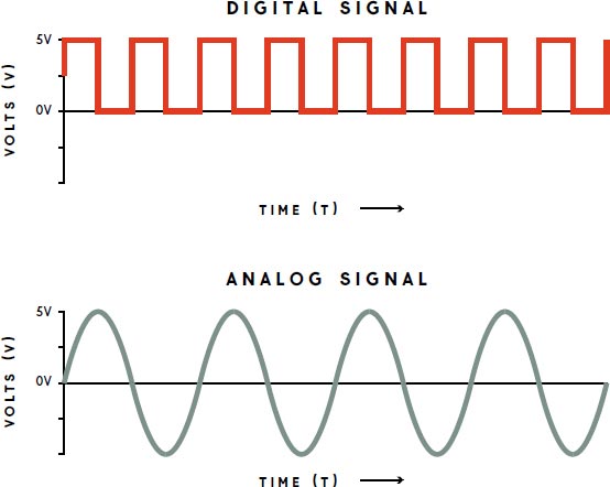
The digital signal is the square wave, which has only two possible values; on corresponds to 5V, and off corresponds to 0V. The analog signal is the sine wave, which transitions smoothly between all the way on and all the way off.

READING VERSUS WRITING DATA

When you fetch data from a sensor or any other Arduino input, you are reading that information. When you send information to a pin, you’re writing to that pin.

There are four Arduino functions that let you read and write analog and digital data:

analogRead()Reads an analog value of a pin

analogWrite()Writes an analog value to a pin

digitalRead()Reads if a pin is on or off

digitalWrite()Turns a pin on or off

You’ve seen digitalWrite() already: you used it to write HIGH and LOW to pin 4 in Listing 13-2, in order to blink LED D4 on the Digital Sandbox.

In this project, you’ll use the analogRead() function to read a sensor value and print that value out over the serial port. The first step is making the data available to your computer.

READING DATA FROM SENSORS

Sensors, like the light sensor and microphone on the Digital Sandbox, output analog data, which you can read with the Arduino. But computers can operate only on digital data! Fortunately, you can write Arduino sketches that send analog data values to your computer as digital data, using serial communication.

Try sending some data from the light sensor on the Digital Sandbox. Start a new Arduino sketch, write the following program, and upload it to the Digital Sandbox:

This little sketch does a lot of cool magic, so let’s unpack it a bit. In the setup() function, you start serial communication with Serial.begin() ❶. You pass begin() the baud rate, which is the speed at which the Sandbox will talk to your computer.

In the loop() function, you create a local variable called val and set it to whatever is read over analog input pin A1 ❷. You then print val over the serial port using the Serial.println() function ❸. Just like in Processing, Arduino’s println() means that there is a carriage return after Arduino prints the value you pass it. Finally, you use the delay() function ❹ to slow the Digital Sandbox down so you can actually read the values when you open the serial port.

Upload this sketch to your Arduino if you haven’t done so already; the TX LED should blink really fast to tell you the board is sending data to your laptop. Next, click the magnifying glass icon in the upper-right corner of the Arduino IDE. The window that opens is called the Serial Monitor, and it allows you to view data being sent over the serial port from the Digital Sandbox. You will see a stream of numbers flying by, as in Figure 13-12. These values are being read from the light sensor labeled A1 on the Digital Sandbox.

FIGURE 13-12: The Arduino Serial Monitor with a single sensor output

Put your hand over the sensor, and the numbers in the Serial Monitor should decrease. The lowest value you will read is 0 (completely dark) and the highest is 1023 (really bright). As you move your hand away from the sensor, the values should grow again. Pretty cool, huh?

These numbers are being transmitted from the Digital Sandbox to your computer over your USB cable. Now you’ve successfully transferred information from one small computer (the Digital Sandbox) to a larger computer, but wait: it gets better.

You can send more than one sensor value to your computer at a time because the Arduino can also send a string of comma-separated values (CSV) over the serial port. That’s important because the more information you can pass to and from Processing, the more control and freedom you have within a project. This capability also allows you to use fewer resources on your computer. Sending one string is much more efficient than sending three separate values, and Processing can easily work with the single string, as you’ve seen in previous projects.

To send multiple values, just change your existing loop as follows:

This version of the loop creates three different variables: light, sound, and temp. These correspond to the three analog sensors you are reading, which are labeled A1, A2, and A0, respectively, on the Digital Sandbox. Next, you print the sensor values over the Serial Monitor with a comma between each pair of values. The final value, temp, is printed with println() so that each set of data appears on a single line, followed by a carriage return. That way, your trios of sensor data won’t run together.

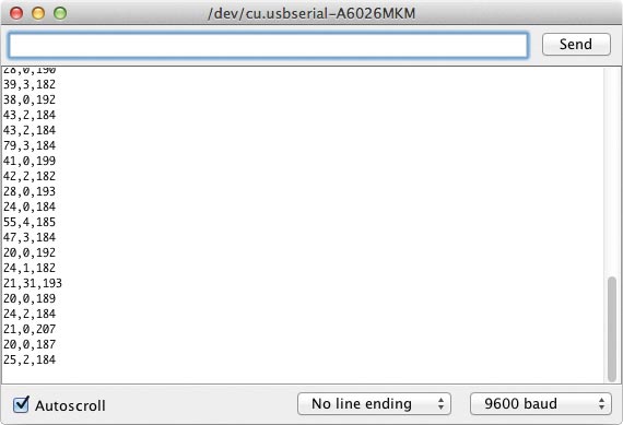
Upload this sketch to your Digital Sandbox and open your Serial Monitor. You should see output similar to Figure 13-13, with sets of three comma-separated values scrolling by.

To change temp (the last value in every trio), place your finger on the temperature sensor. Yell, sing, or just make some noise near the microphone to watch the sound variable (the second value) change. And of course, if you place your hand over the light sensor, the light variable should still change. Save your Arduino sketch now so you don’t lose your work, and then head over to Processing.

FIGURE 13-13: Serial Monitor with sets of three comma-separated values

CREATING THE SENSOR DATA DASHBOARD IN PROCESSING

Your sensor dashboard is half complete: you have three sensor values coming from your Digital Sandbox, and you can see them as a long list of numbers flying by. But those numbers probably don’t tell you much; you can see changes, but it’s hard to picture what they mean.

In this project, you’ll build a dashboard to translate the data coming into your computer through serial communication into helpful visualizations, and then you’ll log that data into a text file for future analysis in a graphing program such as Microsoft Excel or Google Sheets. The Processing sketch you’ll write is a great base for any project that uses serial communication.

Importing Libraries and Creating Variables

First, open a fresh Processing sketch and import the Serial library. This library is native to Processing, so simply click Sketch Import Library . . . Serial. When you see the import line at the top of your sketch, create a class object so you can use functions from the Serial library:

When you used the Video library, you created a Movie object; with the Serial library, you create a Serial object. You’ll use only a single port for this project, so you can just call it myPort.

You’ll also need to create three global variables to receive data from the serial port:

Add three variables with the same names and data types as the sensor variables you created in your Arduino sketch. (Using the same names will help you remember which values in Processing match the values from the Arduino.) These need to be global variables so you can use them in both your draw() loop and in an event function to collect the serial data.

Initialize each variable to 0. This keeps Processing from generating an error the first time it runs through the sketch, since it won’t have a value from the serial port right away.

Preparing Processing for Serial Communication

Next, tackle the setup() function of the sketch, starting with picking a sketch window size. To identify the serial port your Digital Sandbox is on, you can list all possible serial ports on your computer, just like you did for your webcam in Project 10. Add the setup() function in the following listing to your Processing sketch now:

To view the serial ports, pass Serial.list() to the println() function ❶. Next, instantiate your Serial object, myPort ❷. This creates a new Serial object for the port defined by Serial.list()[n] (where n is the index of the port you want to use) at a baud rate of 9600 bits per second (bps).

Finally, at ❸, specify the buffer, which is where Processing stores incoming data from the serial port until you use it. The Serial library’s bufferUntil() function allows you to set a character that Processing uses as a flag or alert. Processing holds (or “buffers”) data until it receives that character, and on receipt, it triggers a call to an event function.

Fetching Your Serial Data

Normally, you’d write the draw() loop now, but you should make sure you can run and receive data from your serial port first. Otherwise, you’ll have no data to create visualizations for! You will insert the draw() loop between the setup and event functions once you know you are receiving data.

Create a serialEvent() function and pass it the Serial object myPort, so the function knows which port to listen on.

Like other event functions, serialEvent() just waits patiently until it’s triggered. When it sees data come in over myPort, it starts capturing the values. Add the following to your event function:

Use the readStringUntil() function ❶ to create a string and store data from the serial port until a newline character (‘ ’) comes through. Once Processing stores the data as inString, you can harvest the usable data. At ❷, an if() statement checks whether your sketch received data by comparing inString to null (or nothing). If inString equals null, then it has no characters. But if there are characters in inString, you tell Processing to trim() any whitespace in the data ❸. (Whitespace refers to blank spaces at the beginning and end of a string.)

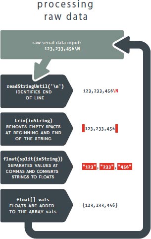
Now you need to break up inString into three pieces of usable data. “Usable” is key: right now, inString contains the temperature, light, and sound data you need, but as a bunch of characters, not numbers!

To fix this, first create a float array called vals ❹. To get the data from inString to vals, you have to do a little inception: putting functions inside functions. When Processing sees nested functions like split() inside of float(), it executes them according to the same order of operations you hated in middle school. The innermost function is performed first, and Processing moves out from there. First, inString is split into pieces of data at every comma in the string. Then, those pieces of data are turned into floats and placed in the vals array. Figure 13-14 shows the conversion process with an example piece of data.

FIGURE 13-14: Progression of preparing and parsing a comma-separated string

The last if() statement ❺ in the event function checks to make sure you have the correct number of values from the serial port. If the vals array has a length of at least 3, map the first three values to numbers that you want to use, and assign the mapped values to temp, light, and sound.

For this sketch, you’ll get a value from 0 to 1023 from the Digital Sandbox, but your sketch window is set to 700 pixels wide by 400 pixels high. To display the sensor values within that area, you need to scale them down. The map() function allows you to take a variable with an expected minimum and maximum and map its values to a different minimum and maximum. You will be creating a bar graph with a maximum height of 200, hence the scale from 0 to 200 ❻.

Here is the syntax for the map() function:

The x argument is the value you need to map, Fmin and Fmax are the original range of values, and Tmin and Tmax are the range you want to map to.

Save your Processing sketch now. That may have looked like a lot of fancy coding, but it’s worth it! Just look at what you’ve done so far. You programmed two different computers—the Digital Sandbox and your computer—to talk to each other. That’s pretty cool!

Testing the Serial Connection

You’ll perform one final check before taking off to draw your dashboard: is your sensor data actually being received correctly in Processing? To find out, call the println() function in a simple draw() loop. Add the following after your existing setup() function, and before the serialEvent() function:

Make sure your Digital Sandbox is plugged in to your computer and the TX LED is blinking. Then, click the Run button in Processing. Depending on your serial port settings, your sketch may just run, or you may get an error that prevents it from doing so, as shown in Figure 13-15.

FIGURE 13-15: Processing shows an error if you get the wrong serial port

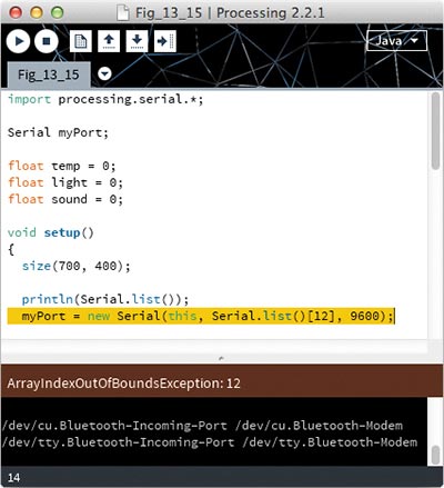
Whether you get an error or not, in your Processing console there should be a list of all available serial ports. If your sketch runs but your console fills with 0.0,0.0,0.0, then you’ve selected a working serial port on your computer, but it may not be connected to the Digital Sandbox. Stop your sketch, click Run, wait 1 second, and quickly stop the sketch again. Scroll to the top of your console, and you should see your list of ports.

You need to select the port that matches the one you used to program your Digital Sandbox. The list is an array, so the first port is 0 and the rest count up from there. Change the 0 in your myPort object to reflect the correct serial port.

Once you change the port number, click the Run button in Processing. A blank sketch window appears, and the console prints strings of three numbers (each ranging from 0 to 200) separated by commas. Those number strings are the scaled values after Processing has mapped the raw values coming over your serial monitor in Arduino. Success!

Play with the sensors, and the values the console window should change as shown in Figure 13-16.

FIGURE 13-16: Sensor values coming from the Digital Sandbox

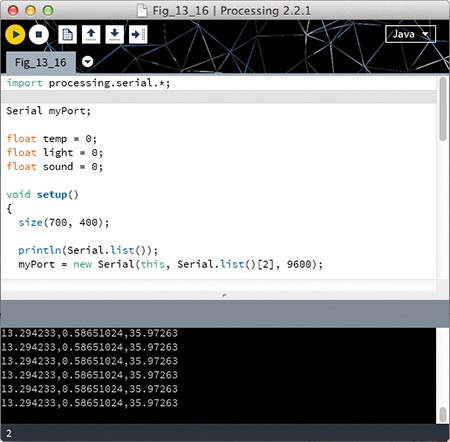
The values are your light, sound, and temperature sensor values. Remember that you mapped these values to 0-200, so some may be lower than the raw 0-1,023 values you are really getting from the Digital Sandbox.

When you know everything works, save your sketch so you don’t lose it, and flesh out your draw() loop.

Visualizing Your Sensor Data

Now that you’re sending sensor data to light, sound, and temp, you can use them just like any other variables in Processing. To demonstrate, let’s make a bar graph to visualize these values.

In the same sketch, draw a few different-colored rectangles, using the three sensor variables to set the height of each:

At ❶, I drew a single line across the entire sketch. This line is your base or zero line for the bar graphs. Then, I called noStroke() to avoid drawing an outline around the graph bars. Following that, I drew three rectangles. Notice that I set the sensor variables to negative ❷ to calculate the height parameter in the up or down direction for each rectangle. This step inverts the rectangle height, since the y-value increases in the downward direction.

Drawing the bars of the bar graphs also reveals why you mapped the values to the range of 0 to 200. If you left the raw values at 0-1,023, your rectangles would extend beyond your sketch and you’d probably rarely see any change. Since you mapped the values to 0-200, the highest bars should be 300 - 200 = 100 pixels from the top of your sketch.

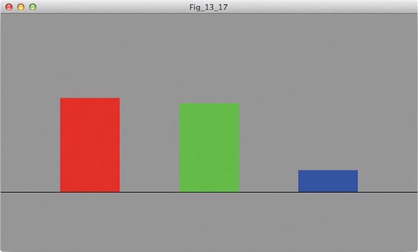
Click Run in Processing, and as the variables change (that is, when you make noise, put your hand over the Digital Sandbox, and so on) you should see the rectangles move up and down. Yay—you can now visualize the change in your variables! See Figure 13-17 for an example.

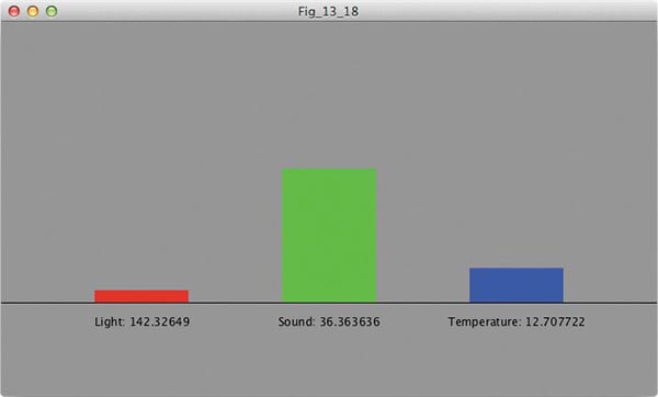
To fully take advantage of the bar graph, label each bar and display the actual number you are graphing. Add the following to your draw() loop now, after the last call to rect() but before the final curly bracket:

FIGURE 13-17: Graphing sensor values (from left to right: light, sound, and temperature)

This code displays the variable name and the live mapped sensor value underneath the bar graph. You now have a completed live dashboard for visualizing data coming in through your serial port connection. Save your sketch and run it, and you should see something like Figure 13-18.

FIGURE 13-18: Sensor graph with printed values

The sky is the limit in terms of what data you can collect using Arduino and then visualize it with Processing!

There are a number of applications for this project in industry, science, and even in your house. In home automation, the ability to collect information about a specific room and display it on a phone or central monitor is a must, and this project is a great foundation for doing that.

If you want to save all of this data and experiment with those kinds of applications later, you simply write the data to a text file. You can do that next.

LOGGING SENSOR DATA WITH PROCESSING

Processing’s PrintWriter class allows you to save data to a text file in your sketch folder, so you can use it to save your sensor data for future use.

First, create a PrintWriter object in your graph project sketch; I called it output:

Then, initialize output in your setup:

Set output with a call to the createWriter() function; then, pass the function a string specifying the name of the text file you want to create. Note the .txt extension in my example, DSInput.txt. You can initialize output anywhere in your setup() function, as long as you do so before you add anything to the text file.

To add information to your text file, print to it with a slightly different println() function. Add the following line to the end of your draw() loop:

This function acts like the println() function you’ve used already, but instead of printing to the console window of the IDE, it prints the data to a text file.

There are a few things you need to do to make this new println() function useful. First, Processing needs to know when you are done printing information so it can flush the buffer, or get rid of the information that is backed up. To tell Processing when you are finished logging data, add a keyPressed() event function after the draw() loop:

When you press the up arrow, this event function tells Processing to flush the buffer and close the text file. The close() function is the most important part. If you never close the text file, it will never be saved or even created in the first place! Checking for a specific key here allows you to add responses to other keys in the future without triggering Processing to close the text file.

With that, you can visualize your data in real time, stockpile it, and analyze and interpret it en masse later. Save your sketch, click Run, allow the sketch to run for a while, and play with the sensors. After about a minute, press the up arrow. Close your sketch window, and open your sketch folder. You will see a text file with the name you passed to createWriter(). Open it, and you will see a list of comma-separated values. These values are the logged values from the time that you ran your sketch. The only caveat to this technique is that every time you run this sketch, use the createWriter() function, and save the text file, it writes over the previous file.

TAKING IT FURTHER

This project was huge in terms of expanding the usefulness of Processing! You learned how to send data to Processing from other devices over a serial connection. You also learned how to log data and save it to a text file. Both of these skills are invaluable, and at SparkFun, we use them on a regular basis.

Try adding an Arduino to another Processing sketch, or modify this one to visualize the data in a more creative way. Look into the other information you can get from the Digital Sandbox; there are a few other inputs you can add, including a button and a switch. How could you harness those in Processing?

NOTE

You can also just download the Processing and Arduino sketches for this section, along with the rest of the source code for this book, at http://www.nostarch.com/sparkfunprocessing/. Open the Project 13 folder, and load RGB.pde in Processing and RGB.ino in Arduino.

One great extension of using the Serial library with Processing is to send data from Processing to a microcontroller, the opposite of what this project did. In this final “Taking It Further,” I’ll give you some Processing code to control the RGB LED on the Digital Sandbox. The RGB is three LEDs in one: a red, green, and blue LED. You can control each individually to do some really cool color mixing and build something like an interactive lamp or light sculpture.

Sending Data from Processing to Arduino

Open a new Processing sketch, and write the following sketch:

This sketch uses the same keyPressed() event function that you used in “Creating a Color-Changing Feedback Box” on page 141, where you changed the color of the lines you drew with your mouse to create a basic graphics application. But instead of using those variables in Processing, this sketch writes r, g, and b across the serial port from Processing to the Arduino.

The sketch follows the same basic structure as the other Serial library sketches you created in this project. The magic happens in the keyPressed() event function and the draw() loop. There are three global variables r, g, and b ❶ (color variables as in Project 8). The setup() function follows the same pattern as in “Preparing Processing for Serial Communication” on page 251.

The draw() loop sets the sketch window background to an RGB setting of r, g, and b ❷, which starts out black. Next, you build a comma-separated string of values (r,g,b) by creating a string called outString. Convert the value of each color variable into a string using the str() function, concatenate the stringified values with comma characters, and finish with a carriage return ❸. Then, write your outString over the serial port ❹. To help you debug your outString, add a println() function that prints the string in the Processing console ❺.

The keyPressed() event function simply reads the key pressed, and if the key is R, G, or B, it increments the appropriate variable. If a variable runs over 255, it is reset to 0. Save your work in Processing, and now let’s work on the Arduino side.

Receiving Processing Data on an Arduino

Open a new Arduino IDE window, select the Fio as your board, and use the same serial port you did in “An Arduino Hello World” on page 243. From this point, copy the following code into the Arduino code window, and upload it to your Digital Sandbox.

First, create three global variables for the red, green, and blue values ❶ that you will later capture from the serial port. At this point, set all three of them to 0.

Next comes the setup() function. Start the Serial library by calling the begin() function, and pass it the baud rate, which is the speed at which the Digital Sandbox will communicate with your Processing sketch ❷. Set pins 9, 10, and 11 as output by passing the pinMode() function the pin numbers and the state at which you will want the pins ❸.

The loop() uses the analogWrite() function to write the three color values, which range from 0 to 255 for each appropriate pin: red is pin 9, green is 10, and blue is 11 ❹. The first time through the loop, these values should all be 0, and the RGB LED should be off.

Next comes an if() statement ❺ that uses Serial.available() to check if there’s anything on the serial port. If there is, this parameter will return 1, so check if it’s greater than 0. If the statement is true, call the Serial.parseInt() function for each color variable. This function reads incoming values as integers until it sees a non-numeric value. In this case, your values are comma-separated, so it will split the values at the comma. Since there are three values, use parseInt() three times to capture each value and set the variables to those values.

Upload this code to your Digital Sandbox, keep the Sandbox plugged in to your computer, run the Processing sketch, and press R, G, or B repeatedly. The Processing sketch window should change color, and the RGB LED on your Digital Sandbox should show a similar color, like in Figure 13-19.

This project was the tip of the iceberg when it comes to devices you can connect to Processing through a serial communication port. For example, I’m a huge fan of DIY identification, and one of my favorite applications is an RFID reader kit we sell (KIT-13198). This kit reads the unique ID string for a card and prints it over the serial port. The uses for RFID are endless, from identifying specific objects and assigning each a different function to personal identification and security.

FIGURE 13-19: The magic RGB LED that you can color-mix to your heart’s content

Now, I send you off into the wild blue yonder of Processing! With the completion of this chapter and this book, you’re well on your way to becoming a full-fledged software developer, digital artist, or interface designer. I hope that this final chapter inspires you to further explore Processing and all the different rabbit holes that you can go down to make useful, beautiful projects. When you need more inspiration, check out the Reference page at Processing.org, look at different libraries, or simply google “Processing projects.” Create something cool and share it with others!