You may be surprised to find a chapter about mathematics in a book aimed at explaining building techniques. However, just as we can’t put programming aside totally, so too we cannot neglect an introduction to some basic mathematical techniques. As we’ve explained, robotics involves many different disciplines, and it’s almost impossible to design a robot without considering its programming issues together with the mechanical aspects. For this reason, some of the projects we are going to describe in this book include sample code, and we want to provide here the basic foundations for the math you will find in that code. Don’t worry’ the math we’ll discuss in this chapter doesn’t require anything more sophisticated than the four basic operations of adding, subtracting, multiplying, and dividing. The first section, about multiplying and dividing, explains in brief how computers deal with integer numbers, focusing on the NXT in particular. This topic is very important, because if you are not familiar with the logic behind computer math, you are bound to run into some unwanted results, which will make your robot behave in unexpected ways.

The three subsequent sections deal with averages, interpolation, and hysteresis, and a fourth explains strategies to deal with more complex calculations. Though averages, interpolation, and hysteresis are not essential, you should consider learning these basic mathematical techniques, because they can make your robot more effective while at the same time keep its programming code simpler. Averages cover those cases where you want a single number to represent a sequence of values. School grades are a good example of this: They are often averaged to express the results of students with a single value (as in a grade point average). Robotics can benefit from averages on many occasions, especially those situations where you don’t want to put too much importance on a single reading from a sensor, but rather observe the tendency shown by a group of spaced readings.

Interpolation deals with the estimating, in numerical terms, the value of an unknown quantity that lies between two known values. Everyday life is full of practical examples— when the minute hand on your watch is between the three and four marks, you interpolate that data and deduce that it means, let’s say, 18 minutes. When a car’s gas gauge reads half a tank, and you know that with the full tank the car can cover about 400 miles, you make the assessment that the car can currently travel approximately 200 miles before needing refueling. Similarly in robotics, you will benefit from interpolation when you want to estimate the time you have to operate a motor in order to set a mechanism in a specific position, or when you want to interpret readings from a sensor that fall between values corresponding to known situations.

The last tool we are going to explore is hysteresis. Hysteresis defines the property of a variable for which its transition from state A to state B follows different rules than its transition from state B to state A. Hysteresis is also a programmed behavior in many automatic control devices because it can improve the efficiency of the system, and it’s this facet that interests us. Think of hysteresis as being similar to the word tolerance, describing, in other words, the amount of fluctuation you allow your system before undertaking a corrective action. The hysteresis section of the chapter will explain how and why you might add hysteresis to the behavior of your robots.

If your robot requires more complex calculations, two simple strategies can simplify the task. The first strategy is to use a type of arithmetic that can represent fractional numbers, not only integers. The second is to rely on existing building blocks from which you can construct more complex calculations, such as NXT-G blocks and RobotC functions that compute trigonometric functions, square roots, and so on.

If you are not an experienced programmer, first of all we want to warn you that in the world of computers, mathematics may be a bit different from what you’ve been taught in school, and some expressions may not result in what you expect. The math you need to know to program the small NXT is no exception.

Computers are generally very good at dealing with integer numbers, that is, whole numbers (1, 2, 3...) with the addition of zero and negative whole numbers. In Chapter 7, we introduced variables, and explained that variables are like boxes aimed at containing numbers. An integer variable is a variable that can contain an integer number. What we didn’t say in Chapter 7 is that variables put limits on the size of the numbers you can store in them, the same way that real boxes can contain only objects that fit inside. You must know and respect these limits; otherwise, your calculations will lead to unexpected results. If you try to pour more water in a glass than what it can contain, the exceeding water will overflow. The same happens to variables if you try to assign them a number that is greater than their capacity— the variable will retain only a part of it.

NXT-G manipulates integer numbers in the range -2,147,483,648 through 2,147,483,647 (a little more than 2 billion). RobotC gives you more options. In the program fragment that follows, the variables a, b, and c can store any integer between -2,147,483,648 and 2,147,483,647 (just like NXT-G numbers). The variables x, y, and z can store only integers between -32,768 and 32,767. The type of the variable determines the range of numbers that it can store: Long variables can store values between -2,147,483,648 and 2,147,483,647, but short variables can store only values between -32,768 and 32,767.

long a,b,c;
short x,y,z;

Why would you declare variables that can represent only a small range of values? Because they use less memory, so there is room for more of them. Usually, there is no need to worry too much about which number type is best: Long is often a good choice because it provides a large range of numbers and because the NXT has plenty of memory for storing numbers. If your program uses very large arrays that never need to store values greater than 32,767 or less than -32,768, you should declare them as short. RobotC even supports floating-point numbers, which can store fractional values, such as 3.14; we discuss these later in this chapter.

Whatever number type you choose, you must keep the results of your calculations inside the range of the type. This rule applies also to any intermediate result, and entails that you learn to be in control of your mathematics. If your numbers are outside this range, your calculations will return incorrect results and your robot will not perform as expected; in technical terms, this means you must know the domain of the numbers you are going to use. Multiplication and division, for different reasons, are the most likely to give you trouble.

Let’s explain this statement with an example. You build a robot that mounts wheels with a circumference of 231mm. Attached to one wheel is a sensor geared to count 105 ticks per each turn of the wheel. Knowing that the sensor reads a count of 385, you want to compute the covered distance. Recall from Chapter 4 that the distance results from the circumference of the wheel multiplied by the number of counts and divided by the counts per turn:

231 × 385/105 = 847

This simple expression has obviously only one proper result: 847. But if you try to compute it in RobotC using short variables, you will find you cannot get that result. If you perform the multiplication first, that is, if the expression were written as follows:

(231 × 385)/105

you get 222! If you try to change the order of the operations this way:

231 × (385/105)

you get 693, which is closer but still wrong! What happened? In the first case, the result of performing the multiplication first (88,935) was outside the upper limit of the allowed range, which is only 32,767. The NXT couldn’t handle it properly and this led to an unexpected result. In the second case, in performing the division operation first, you faced a different problem: The NXT handles only integers, which cannot represent fractions or decimal numbers; the result of 385 / 105 should have been 3 2/3, or 3.66666..., but the processor truncated it to 3 and this explains the result you got.

Unfortunately, there is no general solution to this problem. A dedicated branch of mathematics, called numerical analysis, studies how to limit the side effects of mathematical operations on computers and quantify the expected errors and their propagation along calculations. Numerical analysis teaches that the same error can be expressed in two ways: absolute errors and relative errors. An absolute error is simply the difference between the result you get and the true value. For example, 4355 / 4 should result in 1,088.75; the NXT truncates it to 1,088, and the absolute error is 1,088.75 - 1,088 = 0.75. The division of 7 by 4 leads to the same absolute error: The right result is 1.75, it gets truncated to 1, and the absolute error is again 0.75. To express an error in a relative way, you divide the absolute error by the number to which it refers. Usually, relative errors get converted into percentage errors by multiplying them by 100. The percentage errors of our previous examples are quite different one from the other: 0.07 percent for the first one (0.75 / 1,088.75 × 100) and an impressive 42.85 percent error for the latter (0.75 / 1.75 × 100)! Here are some useful tips to remember from this complex study:

In some situations, you may prefer that your robot base its decisions not on a single sensor reading, but on a group of them, to achieve more stable behavior. For example, if your robot has to navigate a pad composed of colored areas rather than just black and white, you would want it to change its route only when it finds a different color, ignoring transition areas between two adjacent colors (or even dirt particles that could be “read” by accident).

Another case is when you want to measure ambient light, ignoring strong lights and shadows. Averaging provides a simple way to solve these problems.

Simple Averages

You’re probably already familiar with the simple average, the result of adding two or more values and dividing the sum by the number of addends. Let’s say you read three consecutive light values of 65, 68, and 59. Their simple average would be:

(65 + 68 + 59) / 3 = 64

which is expressed in the following formula:

A = (V₁ +V₂+... +V_n)/n

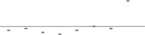
The main property of the average, what actually makes it useful to our purpose, is that it smoothes single peak values. The larger the amount of data averaged, the smaller the effect of a single value on its result. Look at the following sequence:

60, 61, 59, 58, 60, 62, 61, 75

The first seven values fall in the range of 58 to 62, and the eighth one stands out with a 75. The simple average of this series is 62; thus, you see that this last reading doesn’t have a strong influence (see Figure 12.1).

Figure 12.1. How Averaging Smoothes Peaks and Valleys in the Data

In your practical applications, you won’t average all the readings of a sensor, usually just the last n ones. It is like saying you want to benefit from the smoothing property of an average, but you want to consider only more recent data because older readings are no longer relevant.

Every time you read a new value, you discard the oldest one with a technique called the moving average. It’s also known as the boxcar average. Computing a moving average in a program requires you to keep all the last n values stored in variables, and then properly initialize them before the actual execution begins. Think of a sequence of sensor values in a long line. Your “boxcar” is another piece of paper with a rectangular cutout in it, and you can see exactly n consecutive values at any one time. As you move the boxcar along the line of sensor values, you average the readings you see in the cutout. It is clear that as you move the boxcar by one value from left to right along the line, the leftmost value drops off and the rightmost value can be added to the total for the average.

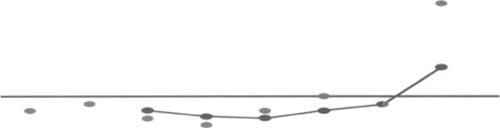
Going back to the series from our previous example, we’ll now show you how to build a moving average for three values. You need the first three numbers to start: 60, 61, and 59. Their average is (60 + 61 + 59) / 3 = 60. When you receive a new value from your sensor, you discard the oldest one (60) and add the newest (58). The average now becomes (61 + 59 + 58) / 3 = 59.333... Figure 12.2 shows what happens to the moving average for three values applied to all the values of the example.

Figure 12.2. A Moving Average for Three Values

When raw data shows a trend, moving averages acknowledge this trend with a “lag.” If the data increases, the average will increase as well, but at a slower pace. The higher the number of values used to compile the average, the longer the lag. Suppose you want to use a moving average for three values in a program. Your RobotC code could be as follows:

long ave, v1, v2, v3;


v2 = SensorValue [SI];
v3 = SensorValue [SI];

while  (true)
{
   vl = v2;
   v2 = v3;
   v3 = SensorValue [SI];
   ave  = (vl+v2+v3) / 3;
   // other  instructions...
}

Note the mechanism in this code that drops the oldest value (vl), replacing it with the subsequent one (v2), and that shifts all the values until the last one is replaced with a fresh reading from the sensor (in v3). The average can be computed through a series of additions and a division.

When the number of readings being averaged is large, you can make your code more efficient using arrays, adopting a trick to improve the computation time and keep the number of operations to a minimum. If you followed the description of the boxcar cutout as it moved along the line, you would realize that the total of the values being averaged did not have to be calculated every time. We just need to subtract the leftmost value, and add the rightmost value to get the new total!

A circular pointer, for example, can be used to address a single element of the array to substitute, without shifting all the others down. The number of additions, meanwhile, can be drastically decreased, keeping the total in a variable, subtracting the value that “exits,” and adding the entering one. The following RobotC code provides an example of how you can implement this technique:

const short SIZE =  3;
long v[SIZE] ;
long i,sum, ave;

// initialize the array
sum = 0 ;
for(i=0;i<SIZE-l;i++)
{
  v[i] = SensorValue[Sl] ;
  sum +=   vii];
}

// first element to assign is the last of the array
i=SIZE-I;
v[i] =0;

// compute moving average
while (true)
{
  sum -= v[i]; //
  v[i] = SensorValue[Sl] ;
  sum += v[i];
  ave = sum /  SIZE;
  i = (i+l) %  SIZE;
  // other instructions...
}

The constant SIZE defines the number of values you want to use in your moving average. In this example, it is set to 3, but you can change it to a different number. The statements that start with long declare the variables; v[SIZE] means that the variable v is an array, a container with multiple “boxes” rather than a single “box.” Each element of the array works exactly like a simple variable, and can be addressed specifying its position in the array. Array elements are numbered starting from 0; thus, in an array with three elements they are numbered 0, 1, and 2. For example, the second element of the array v is v[1].

This program starts initializing the array with readings from the sensor. It uses the for control statement to loop SIZE-1 times, at the same time incrementing the i variable from 0 to SIZE-1. Inside the loop, you assign readings from the sensor to the first SIZE-1 elements of the array. At the same time, you add those values to the sum variable. Supposing that the first readings are 72 and 74; after initialization, v[0] contains 72, v[l] contains 74, and sum contains 146. The initialization process ends assigning to the variable i the number of the first array element to replace, which corresponds to SIZE-1, which is 2 in our example.

Let’s see what happens inside the loop that computes the moving average. Before reading a new value from the sensor, we remove the oldest value from sum. The first time i is 2 and v[i], that is v[2], is 0; thus, sum remains unchanged. v[i] receives a new reading from the sensor and this is added to sum, too. Supposing it is 75, sum now contains 146 + 75 = 221. Now you can compute the average ave, which results in 221 / 3 = 73.666..., and which is truncated to 73. The following instruction prepares the pointer i to the address of the next element that will be replaced. The symbol % in RobotC corresponds to the modulo operator, which returns the remainder of the division. This is what we call a circular pointer, because the expression keeps the value of i in the range from 0 to SIZE-1. It is equivalent to the code:

i = i+l ;
if (i==SIZE) i=O;

which resets i to 0 when it reaches the upper bound. The resulting effect is that i cycles among the values 0, 1, and 2.

During the second loop i is 0, so sum gets decreased to v[0], that is 72, and counts 221 -72 = 149. v[0] is now assigned a new reading—for example, 73—and sum becomes equal to 149 + 73 = 222. The average results 222 / 3 = 74, and i is incremented to l. Then the cycle starts again, and it’s time for v[l] to be replaced with a new value.

This program is definitely much more complicated than the previous one, but it has the advantage of being more general: It can compute moving averages for any number of values by just changing the SIZE constant.

long ave;


// initialize the average
ave = SensorValue[Sl];

// compute average
while (true)
{
  ave = (SensorValue[Sl]  * 20 + ave * 80) / 100;
  // other instructions...
}

ave = (SensorValue[Sl] * 2 + ave * 8) / 10;
ave = (SensorValue[Sl] + ave * 4) / 5;

You’ve built a custom temperature sensor that returns a raw value of 200 at 0° C and 450 at 50° C. What temperature corresponds to a raw value of 315? Your robotic crane takes 10 seconds to lift a load of 100g, and 13 seconds for 200g. How long will it take to lift 180g? To answer these and similar questions, you would turn to interpolation, a class of mathematical tools designed to estimate values from known data.

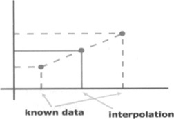
Interpolation has a simple geometric interpretation: If you plot your known data as points on a graph, you can draw a line or a curve that connects them. You then use the points on the line to guess the values that fall inside your data. There are many kinds of interpolation, that is, you can use many different equations corresponding to any possible mathematical curve to interpolate your data. The simplest and most commonly used one is linear interpolation, for which you connect two points with a straight line, and this is what we are going to explain here (see Figure 12.3).

Figure 12.3. Linear Interpolation

Please be aware that many physical systems don’t follow a linear behavior, so linear interpolation will not be the best choice for all situations. However, linear interpolation is usually fine even for nonlinear systems, if you can break down the ranges into almost linear sections.

In following standard terminology, we will call the parameter we change the independent variable, and the one that results from the value of the first, the dependent variable. With a very traditional choice, we will use the letter X for the first and Y for the second. The general equation for linear interpolation is:

(Y - Y_a) / (Y_b - Y_a) = (X - X_a) / (X_b - X_a)

where Y_a is the value ofY we measured for X = X_a and Y_b the one for X_b. With some simple work, we can isolate the Y and transform the previous equation into:

Y = (X - X_a) . (Y_b-Y_a)/(X_b- X_a) ₊ Y_a

This is very simple to use, and allows you to answer your question about the custom temperature sensor. The raw value is your independent variable X, the one you know. The terms of the problem are:

X_a = 200 Y_a = 0

X_b = 450 Y_b = 50

X = 315 Y = ?

We apply the formula and get:

Y = (315 - 200) x (50 - 0) / (450 - 200) + 0 = 23

To make our formula a bit more practical to use, we can transform it again. We define:

m = (Y_b-Y_a)/(X_b-X_a)

If you are familiar with college math, you will recognize in m the slope of the straight line that connects two points. Now our equation becomes:

Y = m × X - m × X_a + Y_a

As X_a and Y_a are known constants, we compute a new term k as:

b = Y_a - m × X_a

So our final equation becomes:

Y = m × X + b

This is the standard equation of a straight line in the Cartesian plane. Looking back to our previous example, you can now compute m and b for your temperature sensor:

m = (50 - 0) / (450 - 200) = 0.2

b = 0 - 0.2 × 200 = -40

Y = 0.2 × X - 40

You can confirm your previous result:

Y = 0.2 × 315-40 = 23

Implementing this equation inside a program for the NXT will require that you convert the decimal value 0.2 into a multiplication and a division, as follows:

temp = (raw * 2) / 10 - 40;

Interpolation is also a good tool when you want to relocate the output from a system in a different range of values. This is what the NXT firmware does when converting raw values from the light and sound sensors into a percentage. You can do the same in your application. Suppose you want to change the way raw values from the light sensor get converted into a percentage. The raw values that the analog sensors return are always in the range 0 to 1,023, but extreme raw values are rare. Let’s say you want to fix an arbitrary range of 900 -> 0 percent and 500 -> 100 percent, and this is what you get from the interpolation formula:

m = (0 - 100) / (900 - 500) = -0.25

b= 100 + 0.25 × 500 = 225

Y= -0.25 × X + 225

Multiplying by 0.25 is like dividing by 4, so we can write this expression in code as:

perc = - raw / 4 + 22 5;

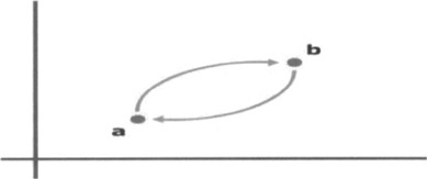
Hysteresis is actually more a physical than a mathematical concept. We say that a system has some hysteresis when it follows a path to go from state A to state B, and a different path when going back from state B to state A. Graphing the state of the system on a chart shows two different curves that connect the points A and B, one for going out and one for coming back (see Figure 12.4).

Figure 12.4. Hysteresis in Physical Systems

Hysteresis is a common property of many natural phenomena, magnetism above all, but our interest here is in introducing some hysteresis in our robotics programs. Why should you do it? First of all, let us say this is quite a common practice. In fact, many automation devices based on some kind of feedback have been equipped with artificial hysteresis.

A very handy example comes from the thermostat that controls the heating in your house. Imagine that your heating system relies on a thermostat designed to maintain an exact temperature, and that during a cold winter you program your desired home temperature to 21° C (70° F). As soon as the ambient temperature goes below 21° C, the heater starts. In a few minutes, the temperature reaches 21° C and the heater stops, then a few minutes later it starts again, and so on, all day long. The heater would turn off and on constantly as the temperature varies around that exact point. This approach is not the best one, because every start phase requires some time to bring the system to its maximum efficiency, just about when it gets stopped again. In introducing some hysteresis, the system can run more smoothly: We can let the temperature go down to 20.5° C, and then heat up the house until it reaches 21.5° C. When the temperature in the house is 21° C, the heater can be either on or off, depending on whether it’s going from on to off or vice versa.

Hysteresis can reduce the number of corrective actions a system has to take, thus improving stability and efficiency at the price of some tolerance. Autopilots for boats and planes are another good example. Could you think of a task for your robots that could benefit from hysteresis? Line following is a good example.

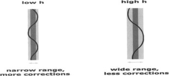
In Chapter 4, in talking about light sensors, we explained that the best way to follow a strip on the floor is to actually follow one of its edges, the borderline between white and black. In that area, your sensor will read a “gray” value, some intermediate number between the white and black readings. Having chosen that value for gray, a robot with no hysteresis may correct left when the reading is greater than gray and right when the reading is less than gray. To introduce some hysteresis, you can tell your robot to turn left when reading gray+h and right when reading gray-h, where h is a constant properly chosen to optimize the performance of your robot. There isn’t a general rule that is valid for any system; you must find the optimal value for h by experimenting: Start with a value of about 1 /6 or 1 /8 of the total white-black difference. This way, the interval gray-h to gray+h will cover 1/3 or 1/4 of the total range. Then start increasing or decreasing its value, observing what happens to your robot, until you are happy with its behavior. You will discover that by reducing h your robot will narrow the range of its oscillations, but will perform more frequent corrections. Increasing h, on the other hand, will make your robot perform fewer corrections but with oscillations of larger amplitude (see Figure 12.5).

Figure 12.5. How Hysteresis Affects Line Following

We suggest a simple experiment that will help you put these concepts into practice by building a real sensor setup that you can manipulate by hand to get a feel for how the robot would behave. Write a simple program that plays tones to ask you to turn left or right. For example, it can beep high when you have to turn left and low to turn right. The RobotC code that follows shows a possible implementation:

const long GRAY = 50;
const long H    = 3 ;

task main()
{
  SetSensorType(SI, sensorLightActive);

  while (true)
  {
    if (SensorValue [SI] >GRAY+H)
      PlayTone(440,20) ;
    else if (SensorValue[Sl]<GRAY-H)
      PlayTone(1760,20) ;
    waitl0Msec (2) ;
  }
}

Equip your NXT with a light sensor attached to input port 1 and you are ready to go. You should tune the value of the GRAY constant to what your sensor actually reads when placed exactly over the borderline between the white and the black. When the program runs, you can move the sensor toward or away from the line until you hear the beep that asks you to correct the direction (keep the sensor always at the same distance from the pad). Experiment with different values for H to see how the accepted range of readings gets wider or narrower.

If you keep a pencil in your hand together with the light sensor, you can even perform this experiment blindfolded! Try to follow the line by just listening to the “instructions” coming from your NXT and compare the lines drawn by your pencil for different values of H.

Robots perform mathematical computations for two reasons: to understand the world around them and to plan their actions. Consider a robot that seeks a certain object—say, a blue ball. The robot uses its sensors to obtain information about the world around it and about its own position. It uses this information to try to estimate where the blue ball is and where it is. Once the robot decides where the ball is and where it is, it needs to plan how to reach the ball. If the environment contains obstacles (such as walls or other robots), finding a path may be a challenging task that requires interesting computations. In some robots, the estimation and planning are simple and require no math or just a bit of math. But a robot may require more sophisticated calculations than we have shown in this chapter.

Integers are not always suitable for complex mathematical calculations, because integer division can generate absolute errors of up to ±1/2, which may be too high. For example, dividing 301 by 2 gives the integer 150, whereas the exact answer is 150 1/2. Computers use several other number types to reduce these errors. The most important noninteger number types are fixed-point numbers and floating-point numbers. We explain these number types with decimal examples, but keep in mind that computers always represent numbers in binary format (base 2). Suppose that each word in the computers memory can store a number with a sign and four decimal digits, and suppose that a certain word stores the digits 3759. In an integer, the decimal point is to the right of the rightmost digit, so if we view these digits as an integer, the number that the word represents is 3,759.0. We can also decide that the decimal point is at some arbitrary fixed position, such as between the second and third digits. The computer stores exactly the same information, but now the word in memory represents 37.59. This is called a fixed-point representation. In fixed point, we cannot represent very large numbers, but we have more accuracy. For example, fixed-point numbers are ideal for averaging sensor readings in percentage mode. On the one hand, the readings (and the averages) never exceed 100, so we never need very large numbers, and on the other hand, fixed-point numbers allow us to represent fractional averages more accurately than integers. To view the digits stored in a memory word as a floating-point number, we split the digits into two groups, a fraction and an exponent. Let’s assume that we use the three leftmost digits as a fraction and the last digit as an exponent. In this case, our memory word would represent the number 0.375 X 10⁹, or 375,000,000. We now have less accuracy, because our numbers have only three significant digits, but we have a much larger range of numbers: These four decimal digits allow us to represent numbers that approach 1 billion.

The processor in every desktop or laptop computer can perform arithmetic on both integers and floating-point numbers very quickly. Therefore, complex mathematical calculations that can produce noninteger results are usually performed on such computers using floating-point arithmetic. The processor of the NXT can perform only integer arithmetic. It can be programmed to perform floating-point arithmetic, but then the arithmetic operations are carried out in software, so they are fairly slow. RobotC supports floating-point calculations in this way. Neither the NXT nor your PC supports fixed-point arithmetic in the processor itself, but fixed-point arithmetic that is implemented in software is only slightly slower than integer arithmetic. Therefore, fixed-point arithmetic is a good choice for performing more complex calculations on the NXT.

Addition and subtraction on fixed-point numbers are performed as though they were integers. For example, 37.59 + 0.63 = 38.22; we can obtain this result by adding 3,759 + 63, which gives 3,822. In other words, for addition and subtraction, it does not matter where the point is, as long as it is in the same fixed positions in all the numbers. Multiplication and division are a bit more complex. The product 37.59 x 0.63 should give 23.6817, but the integer product 3,759 X 63 gives 236,817. To get the correct answer, we need to multiply the input numbers as though they were integers, and then shift the integer product to the right by two digits (because our fixed-point numbers have two digits to the right of the point). This truncates the digits 17 and gives 2368, which we interpret as 23.68, which is the correct fixed-point answer. The answer is not exact, but then there is really no way to represent the 23.6817 with only four decimal digits! Fixed-point multiplication done this way can easily overflow, so you need to either temporarily store the integer product in a number type with more digits (say, long rather than short), or to resort to a more complex multiplication algorithm. Division is somewhat similar to multiplication: To get the correct fixed-point answer, you need to shift the dividend to the left before you divide them by integers. For example, the integer division 375,900 / 63 gives 5,966, which is the correct fixed-point representation of 37.59 / 0.63 = 59.66. Here too you need a temporary variable with more digits.

Fixed-point arithmetic allows you to strike the right balance between accuracy and range, and it is just a bit slower than integer arithmetic. Floating-point arithmetic is even more convenient than fixed-point, because the computer chooses the right range for you after every arithmetic operation, but it is not more accurate and it is slow on the NXT (and is not available at all in NXT-G). Use integers if the accuracy is good enough for you, use fixed-point if you need more accuracy, and use floating-point if speed is not important, you need the convenience, and your programming environment supports floating-point.

Another point to keep in mind if your robot must perform sophisticated calculations is that software components are available that can help you implement these calculations. For example, there are MyBlock and third-party native blocks that compute square roots and trigonometric functions, such as sine and cosine. RobotC also includes functions that compute these functions. As time goes by, more and more such building blocks will become available, both for NXT-G and for RobotC. Expressing calculations in terms of preexisting building blocks simplifies programming considerably; this is how virtually any complex piece of software is built.

Math is the kind of subject that people either love or hate. If you fall in the latter group, we can’t blame you for having skipped most of the content of this chapter. Don’t worry; there was nothing you can’t live without. Just make an effort to understand the part about multiplication and division, because if you ignore the possible side effects, you could end up with some bad surprises in your calculations.

Consider the other topics—averages, interpolation, and hysteresis—to be like tools in your toolbox. Averages are a useful instrument to soften the differences between single readings and to ignore temporary peaks. They allow you to group a set of readings and consider it as a single value. When you are dealing with a flow of data coming from a sensor, the moving average is the right tool to process the last n readings. The larger n is, the more the smoothing effect on the data.

Weighted averages have an advantage over simple averages in that they can show the trend in the data: You can assign the weights to put more importance on more recent data. Exponential smoothing is a special case of weighted averages, the results of which are particularly convenient on the implementation side, because they allow you to write compact and efficient code.

The interpolation technique proves useful when you want to estimate the value of a quantity that falls between two known limits. We described linear interpolation, which corresponds to tracing a straight line across two points in a graph. You then can use that line to calculate any value in the interval.

Hysteresis, a concept borrowed from physics, will help you in reducing the number of corrections your robots have to make to keep within a required behavior. By adding some hysteresis to your algorithms, your robots will be less reactive to changes. Hysteresis can also increase the efficiency of your system.

Some robots may require more sophisticated calculations. This may involve using fixed-point or floating-point numbers and more complex mathematical calculations. If your robot needs complex calculations, try to find building blocks that perform parts of the computation. These building blocks can include MyBlock and third-party blocks that others have made available, or library functions in textual programming languages.

It’s not necessary that you remember all the equations, just what they’re useful for! You can always refer back to the text when you find a problem that might benefit from a mathematical tool that you read about.