
Chapter 7. Search-based applications
This chapter covers
- Searching in Redis
- Scoring your search results
- Ad targeting
- Job search
Over the last several chapters, I’ve introduced a variety of topics and problems that can be solved with Redis. Redis is particularly handy in solving a class of problems that I generally refer to as search-based problems. These types of problems primarily involve the use of SET and ZSET intersection, union, and difference operations to find items that match a specified criteria.
In this chapter, I’ll introduce the concept of searching for content with Redis SETs. We’ll then talk about scoring and sorting our search results based on a few different options. After getting all of the basics out of the way, we’ll dig into creating an ad-targeting engine using Redis, based on what we know about search. Before finishing the chapter, we’ll talk about a method for matching or exceeding a set of requirements as a part of job searching.
Overall, the set of problems in this chapter will show you how to search and filter data quickly and will expand your knowledge of techniques that you can use to organize and search your own information. First, let’s talk about what we mean by searching in Redis.
7.1. Searching in Redis
In a text editor or word processor, when you want to search for a word or phrase, the software will scan the document for that word or phrase. If you’ve ever used grep in Linux, Unix, or OS X, or if you’ve used Windows’ built-in file search capability to find files with words or phrases, you’ve noticed that as the number and size of documents to be searched increases, it takes longer to search your files.
Unlike searching our local computer, searching for web pages or other content on the web is very fast, despite the significantly larger size and number of documents. In this section, we’ll examine how we can change the way we think about searching through data, and subsequently reduce search times over almost any kind of word or keyword-based content search with Redis.
As part of their effort to help their customers find help in solving their problems, Fake Garage Startup has created a knowledge base of troubleshooting articles for user support. As the number and variety of articles has increased over the last few months, the previous database-backed search has slowed substantially, and it’s time to come up with a method to search over these documents quickly. We’ve decided to use Redis, because it has all of the functionality necessary to build a content search engine.
Our first step is to talk about how it’s even possible for us to search so much faster than scanning documents word by word.
7.1.1. Basic search theory
Searching for words in documents faster than scanning over them requires preprocessing the documents in advance. This preprocessing step is generally known as indexing, and the structures that we create are called inverted indexes. In the search world, inverted indexes are well known and are the underlying structure for almost every search engine that we’ve used on the internet. In a lot of ways, we can think of this process as producing something similar to the index at the end of this book. We create inverted indexes in Redis primarily because Redis has native structures that are ideally suited for inverted indexes: the SET and ZSET.[1]
1 Though SETs and ZSETs could be emulated with a properly structured table and unique index in a relational database, emulating a SET or ZSET intersection, union, or difference using SQL for more than a few terms is cumbersome.
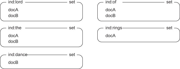
More specifically, an inverted index of a collection of documents will take the words from each of the documents and create tables that say which documents contain what words. So if we have two documents, docA and docB, containing just the titles lord of the rings and lord of the dance, respectively, we’ll create a SET in Redis for lord that contains both docA and docB. This signifies that both docA and docB contain the word lord. The full inverted index for our two documents appears in figure 7.1.
Figure 7.1. The inverted index for docA and docB
Knowing that the ultimate result of our index operation is a collection of Redis SETs is helpful, but it’s also important to know how we get to those SETs.
Basic indexing
In order to construct our SETs of documents, we must first examine our documents for words. The process of extracting words from documents is known as parsing and tokenization; we’re producing a set of tokens (or words) that identify the document.
There are many different ways of producing tokens. The methods used for web pages could be different from methods used for rows in a relational database, or from documents from a document store. We’ll keep it simple and consider words of alphabetic characters and apostrophes (') that are at least two characters long. This accounts for the majority of words in the English language, except for I and a, which we’ll ignore.
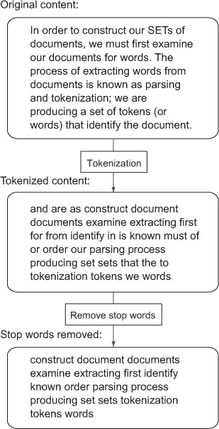
One common addition to a tokenization process is the removal of words known as stop words. Stop words are words that occur so frequently in documents that they don’t offer a substantial amount of information, and searching for those words returns too many documents to be useful. By removing stop words, not only can we improve the performance of our searches, but we can also reduce the size of our index. Figure 7.2 shows the process of tokenization and stop word removal.
Figure 7.2. The process of tokenizing text into words, then removing stop words, as run on a paragraph from an early version of this section
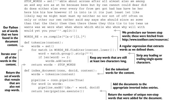
One challenge in this process is coming up with a useful list of stop words. Every group of documents will have different statistics on what words are most common, which may or may not affect stop words. As part of listing 7.1, we include a list of stop words (fetched from http://www.textfixer.com/resources/), as well as functions to both tokenize and index a document, taking into consideration the stop words that we want to remove.
Listing 7.1. Functions to tokenize and index a document
If we were to run our earlier docA and docB examples through the updated tokenization and indexing step in listing 7.1, instead of having the five SETs corresponding to lord, of, the, rings, and dance, we’d only have lord, rings, and dance, because of and the are both stop words.
Removing a document from the index
If you’re in a situation where your document may have its content changed over time, you’ll want to add functionality to automatically remove the document from the index prior to reindexing the item, or a method to intelligently update only those inverted indexes that the document should be added or removed from. A simple way of doing this would be to use the SET command to update a key with a JSON-encoded list of words that the document had been indexed under, along with a bit of code to un-index as necessary at the start of index_document().
Now that we have a way of generating inverted indexes for our knowledge base documents, let’s look at how we can search our documents.
Basic searching
Searching the index for a single word is easy: we fetch the set of documents in that word’s SET. But what if we wanted to find documents that contained two or more words? We could fetch the SETs of documents for all of those words, and then try to find those documents that are in all of the SETs, but as we discussed in chapter 3, there are two commands in Redis that do this directly: SINTER and SINTERSTORE. Both commands will discover the items that are in all of the provided SETs and, for our example, will discover the SET of documents that contain all of the words.
One of the amazing things about using inverted indexes with SET intersections is not so much what we can find (the documents we’re looking for), and it’s not even how quickly it can find the results—it’s how much information the search completely ignores. When searching text the way a text editor does, a lot of useless data gets examined. But with inverted indexes, we already know what documents have each individual word, and it’s only a matter of filtering through the documents that have all of the words we’re looking for.
Sometimes we want to search for items with similar meanings and have them considered the same, which we call synonyms (at least in this context). To handle that situation, we could again fetch all of the document SETs for those words and find all of the unique documents, or we could use another built-in Redis operation: SUNION or SUNIONSTORE.
Occasionally, there are times when we want to search for documents with certain words or phrases, but we want to remove documents that have other words. There are also Redis SET operations for that: SDIFF and SDIFFSTORE.
With Redis SET operations and a bit of helper code, we can perform arbitrarily intricate word queries over our documents. Listing 7.2 provides a group of helper functions that will perform SET intersections, unions, and differences over the given words, storing them in temporary SETs with an expiration time that defaults to 30 seconds.
Listing 7.2. SET intersection, union, and difference operation helpers
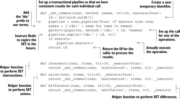
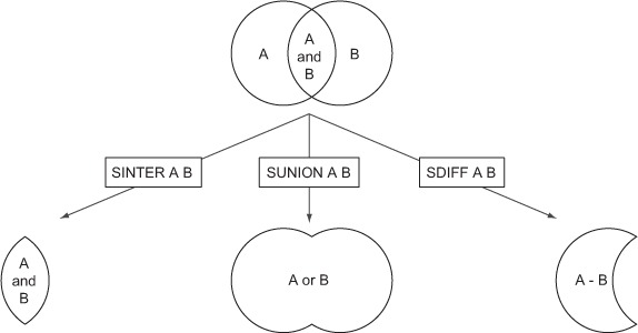
Each of the intersect(), union(), and difference() functions calls another helper function that actually does all of the heavy lifting. This is because they all essentially do the same thing: set up the keys, make the appropriate SET call, update the expiration, and return the new SET’s ID. Another way of visualizing what happens when we perform the three different SET operations SINTER, SUNION, and SDIFF can be seen in figure 7.3, which shows the equivalent operations on Venn diagrams.
Figure 7.3. The SET intersection, union, and difference calls as if they were operating on Venn diagrams
This is everything necessary for programming the search engine, but what about parsing a search query?
Parsing and executing a search
We almost have all of the pieces necessary to perform indexing and search. We have tokenization, indexing, and the basic functions for intersection, union, and differences. The remaining piece is to take a text query and turn it into a search operation. Like our earlier tokenization of documents, there are many ways to tokenize search queries. We’ll use a method that allows for searching for documents that contain all of the provided words, supporting both synonyms and unwanted words.
A basic search will be about finding documents that contain all of the provided words. If we have just a list of words, that’s a simple intersect() call. In the case where we want to remove unwanted words, we’ll say that any word with a leading minus character (-) will be removed with difference(). To handle synonyms, we need a way of saying “This word is a synonym,” which we’ll denote by the use of the plus (+) character prefix on a word. If we see a plus character leading a word, it’s considered a synonym of the word that came just before it (skipping over any unwanted words), and we’ll group synonyms together to perform a union() prior to the higher-level intersect() call.
Putting it all together where + denotes synonyms and - denotes unwanted words, the next listing shows the code for parsing a query into a Python list of lists that describes words that should be considered the same, and a list of words that are unwanted.
Listing 7.3. A function for parsing a search query

To give this parsing function a bit of exercise, let’s say that we wanted to search our knowledge base for chat connection issues. What we really want to search for is an article with connect, connection, disconnect, or disconnection, along with chat, but because we aren’t using a proxy, we want to skip any documents that include proxy or proxies. Here’s an example interaction that shows the query (formatted into groups for easier reading):
>>> parse('''
connect +connection +disconnect +disconnection
chat
-proxy -proxies''')
([['disconnection', 'connection', 'disconnect', 'connect'], ['chat']],
['proxies', 'proxy'])
>>>
Our parse function properly extracted the synonyms for connect/disconnect, kept chat separate, and discovered our unwanted proxy and proxies. We aren’t going to be passing that parsed result around (except for maybe debugging as necessary), but instead are going to be calling our parse() function as part of a parse_and_search() function that union()s the individual synonym lists as necessary, intersect()ing the final list, and removing the unwanted words with difference() as necessary. The full parse_and_search() function is shown in the next listing.
Listing 7.4. A function to parse a query and search documents
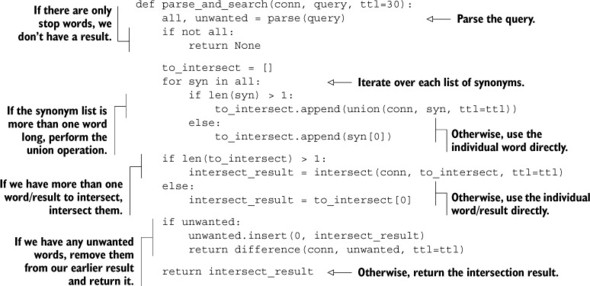
Like before, the final result will be the ID of a SET that includes the documents that match the parameters of our search. Assuming that Fake Garage Startup has properly indexed all of their documents using our earlier index_document() function, parse_and_search() will perform the requested search.
We now have a method that’s able to search for documents with a given set of criteria. But ultimately, when there are a large number of documents, we want to see them in a specific order. To do that, we need to learn how to sort the results of our searches.
7.1.2. Sorting search results
We now have the ability to arbitrarily search for words in our indexed documents. But searching is only the first step in retrieving information that we’re looking for. After we have a list of documents, we need to decide what’s important enough about each of the documents to determine its position relative to other matching documents. This question is generally known as relevance in the search world, and one way of determining whether one article is more relevant than another is which article has been updated more recently. Let’s see how we could include this as part of our search results.
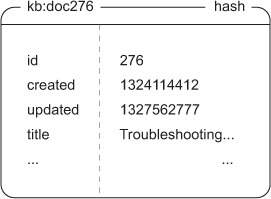
If you remember from chapter 3, the Redis SORT call allows us to sort the contents of a LIST or SET, possibly referencing external data. For each article in Fake Garage Startup’s knowledge base, we’ll also include a HASH that stores information about the article. The information we’ll store about the article includes the title, the creation timestamp, the timestamp for when the article was last updated, and the document’s ID. An example document appears in figure 7.4.
Figure 7.4. An example document stored in a HASH
With documents stored in this format, we can then use the SORT command to sort by one of a few different attributes. We’ve been giving our result SETs expiration times as a way of cleaning them out shortly after we’ve finished using them. But for our final SORTed result, we could keep that result around longer, while at the same time allowing for the ability to re-sort, and even paginate over the results without having to perform the search again. Our function for integrating this kind of caching and re-sorting can be seen in the following listing.
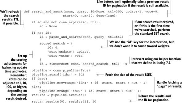
Listing 7.5. A function to parse and search, sorting the results
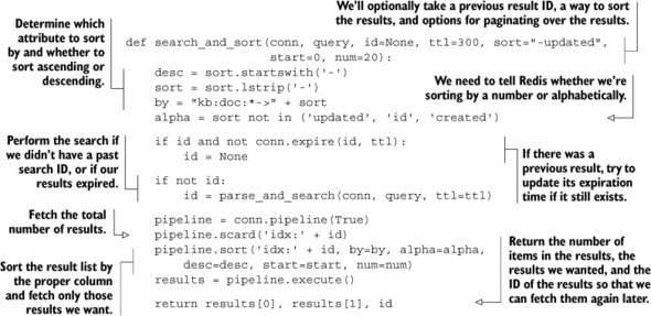
When searching and sorting, we can paginate over results by updating the start and num arguments; alter the sorting attribute (and order) with the sort argument; cache the results for longer or shorter with the ttl argument; and reference previous search results (to save time) with the id argument.
Though these functions won’t let us create a search engine to compete with Google, this problem and solution are what brought me to use Redis in the first place. Limitations on SORT lead to using ZSETs to support more intricate forms of document sorting, including combining scores for a composite sort order.
7.2. Sorted indexes
In the previous section, we talked primarily about searching, with the ability to sort results by referencing data stored in HASHes. This kind of sorting works well when we have a string or number that represents the actual sort order we’re interested in. But what if our sort order is a composite of a few different scores? In this section, we’ll talk about ways to combine multiple scores using SETs and ZSETs, which can offer greater flexibility than calling SORT.
Stepping back for a moment, when we used SORT and fetched data to sort by from HASHes, the HASHes behaved much like rows in a relational database. If we were to instead pull all of the updated times for our articles into a ZSET, we could similarly order our articles by updated times by intersecting our earlier result SET with our update time ZSET with ZINTERSTORE, using an aggregate of MAX. This works because SETs can participate as part of a ZSET intersection or union as though every element has a score of 1.
7.2.1. Sorting search results with ZSETs
As we saw in chapter 1 and talked about in chapter 3, SETs can actually be provided as arguments to the ZSET commands ZINTERSTORE and ZUNIONSTORE. When we pass SETs to these commands, Redis will consider the SET members to have scores of 1. For now, we aren’t going to worry about the scores of SETs in our operations, but we will later.
In this section, we’ll talk about using SETs and ZSETs together for a two-part search-and-sort operation. When you’ve finished reading this section, you’ll understand why and how we’d want to combine scores together as part of a document search.
Let’s consider a situation in which we’ve already performed a search and have our result SET. We can sort our results with the SORT command, but that means we can only sort based on a single value at a time. Being able to easily sort by a single value is one of the reasons why we started out sorting with our indexes in the first place.
But say that we want to add the ability to vote on our knowledge base articles to indicate if they were useful. We could put the vote count in the article hash and use SORT as we did before. That’s reasonable. But what if we also wanted to sort based on a combination of recency and votes? We could do as we did in chapter 1 and predefine the score increase for each vote. But if we don’t have enough information about how much scores should increase with each vote, then picking a score early on will force us to have to recalculate later when we find the right number.
Instead, we’ll keep a ZSET of the times that articles were last updated, as well as a ZSET for the number of votes that an article has received. Both will use the article IDs of the knowledge base articles as members of the ZSETs, with update times or vote count as scores, respectively. We’ll also pass similar arguments to an updated search_and_zsort() function defined in the next listing, in order to calculate the resulting sort order for only update times, only vote counts, or almost any relative balance between the two.
Listing 7.6. An updated function to search and sort based on votes and updated times
Our search_and_zsort() works much like the earlier search_and_sort(), differing primarily in how we sort/order our results. Rather than calling SORT, we perform a ZINTERSTORE operation, balancing the search result SET, the updated time ZSET, and the vote ZSET.
As part of search_and_zsort(), we used a helper function for handling the creation of a temporary ID, the ZINTERSTORE call, and setting the expiration time of the result ZSET. The zintersect() and zunion() helper functions are shown next.
Listing 7.7. Some helper functions for performing ZSET intersections and unions
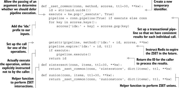
These helper functions are similar to our SET-based helpers, the primary difference being that we’re passing a dictionary through to specify scores, so we need to do more work to properly prefix all of our input keys.
In this section, we used ZSETs to handle combining a time and a vote count for an article. You remember that we did much the same thing back in chapter 1 without search, though we did handle groups of articles. Can you update article_vote(), post_articles(), get_articles(), and get_group_articles() to use this new method so that we can update our score per vote whenever we want?
In this section, we talked about how to combine SETs and ZSETs to calculate a simple composite score based on vote count and updated time. Though we used 2 ZSETs as sources for scores, there’s no reason why we couldn’t have used 1 or 100. It’s all a question of what we want to calculate.
If we try to fully replace SORT and HASHes with the more flexible ZSET, we run into one problem almost immediately: scores in ZSETs must be floating-point numbers. But we can handle this issue in many cases by converting our non-numeric data to numbers.
7.2.2. Non-numeric sorting with ZSETs
Typical comparison operations between strings will examine two strings character by character until one character is different, one string runs out of characters, or until they’re found to be equal. In order to offer the same sort of functionality with string data, we need to turn strings into numbers. In this section, we’ll talk about methods of converting strings into numbers that can be used with Redis ZSETs in order to sort based on string prefixes. After reading this section, you should be able to sort your ZSET search results with strings.
Our first step in translating strings into numbers is understanding the limitations of what we can do. Because Redis uses IEEE 754 double-precision floating-point values to store scores, we’re limited to at most 64 bits worth of storage. Due to some subtleties in the way doubles represent numbers, we can’t use all 64 bits. Technically, we could use more than the equivalent of 63 bits, but that doesn’t buy us significantly more than 63 bits, and for our case, we’ll only use 48 bits for the sake of simplicity. Using 48 bits limits us to prefixes of 6 bytes on our data, which is often sufficient.
To convert our string into an integer, we’ll trim our string down to six characters (as necessary), converting each character into its ASCII value. We’ll then extend the values to six entries for strings shorter than six characters. Finally, we’ll combine all of the values into an integer. Our code for converting a string into a score can be seen next.
Listing 7.8. A function to turn a string into a numeric score
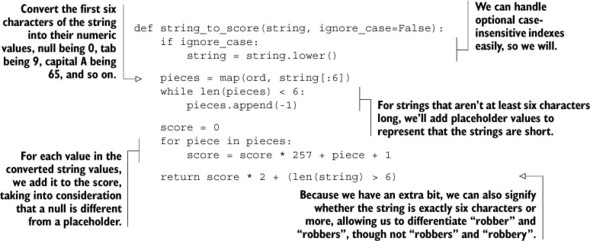
Most of our string_to_score() function should be straightforward, except for maybe our use of -1 as a filler value for strings shorter than six characters, and our use of 257 as a multiplier before adding each character value to the score. For many applications, being able to differentiate between hello\0 and hello can be important, so we take steps to differentiate the two, primarily by adding 1 to all ASCII values (making null 1), and using 0 (-1 + 1) as a filler value for short strings. As a bonus, we use an extra bit to tell us whether a string is more than six characters long, which helps us with similar six-character prefixes.[2]
2 If we didn’t care about differentiating between hello\0 and hello, then we wouldn’t need the filler. If we didn’t need the filler, we could replace our multiplier of 257 with 256 and get rid of the +1 adjustment. But with the filler, we actually use .0337 additional bits to let us differentiate short strings from strings that have nulls. And when combined with the extra bit we used to distinguish whether we have strings longer than six characters, we actually use 49.0337 total bits.
By mapping strings to scores, we’re able to get a prefix comparison of a little more than the first six characters of our string. For non-numeric data, this is more or less what we can reasonably do without performing extensive numeric gymnastics, and without running into issues with how a non-Python library transfers large integers (that may or may not have been converted to a double).
When using scores derived from strings, the scores aren’t always useful for combining with other scores and are typically only useful for defining a single sort order. Note that this is because the score that we produced from the string doesn’t really mean anything, aside from defining a sort order.
Back in section 6.1.2, we used ZSETs with scores set to 0 to allow us to perform prefix matching on user names. We had to add items to the ZSET and either use WATCH/MULTI/EXEC or the lock that we covered in section 6.2 to make sure that we fetched the correct range. But if instead we added names with scores being the result of string_to_score() on the name itself, we could bypass the use of WATCH/ MULTI/EXEC and locks when someone is looking for a prefix of at most six characters by using ZRANGEBYSCORE, with the endpoints we had calculated before being converted into scores as just demonstrated. Try rewriting our find_prefix_range() and autocomplete_on_prefix() functions to use ZRANGEBYSCORE instead.
In this section and for the previous exercise, we converted arbitrary binary strings to scores, which limited us to six-character prefixes. By reducing the number of valid characters in our input strings, we don’t need to use a full 8+ bits per input character. Try to come up with a method that would allow us to use more than a six-character prefix if we only needed to autocomplete on lowercase alphabetic characters.
Now that we can sort on arbitrary data, and you’ve seen how to use weights to adjust and combine numeric data, you’re ready to read about how we can use Redis SETs and ZSETs to target ads.
7.3. Ad targeting
On countless websites around the internet, we see advertisements in the form of text snippets, images, and videos. Those ads exist as a method of paying website owners for their service—whether it’s search results, information about travel destinations, or even finding the definition of a word.
In this section, we’ll talk about using SETs and ZSETs to implement an ad-targeting engine. When you finish reading this section, you’ll have at least a basic understanding of how to build an ad-serving platform using Redis. Though there are a variety of ways to build an ad-targeting engine without Redis (custom solutions written with C++, Java, or C# are common), building an ad-targeting engine with Redis is one of the quickest methods to get an ad network running.
If you’ve been reading these chapters sequentially, you’ve seen a variety of problems and solutions, almost all of which were simplified versions of much larger projects and problems. But in this section, we won’t be simplifying anything. We’ll build an almost-complete ad-serving platform based on software that I built and ran in a production setting for a number of months. The only major missing parts are the web server, ads, and traffic.
Before we get into building the ad server itself, let’s first talk about what an ad server is and does.
7.3.1. What’s an ad server?
When we talk about an ad server, what we really mean is a sometimes-small, but sophisticated piece of technology. Whenever we visit a web page with an ad, either the web server itself or our web browser makes a request to a remote server for that ad. This ad server will be provided a variety of information about how to find an ad that can earn the most money through clicks, views, or actions (I’ll explain these shortly).
In order to choose a specific ad, our server must be provided with targeting parameters. Servers will typically receive at least basic information about the viewer’s location (based on our IP address at minimum, and occasionally based on GPS information from our phone or computer), what operating system and web browser we’re using, maybe the content of the page we’re on, and maybe the last few pages we’ve visited on the current website.
We’ll focus on building an ad-targeting platform that has a small amount of basic information about viewer location and the content of the page visited. After we’ve seen how to pick an ad from this information, we can add other targeting parameters later.
Ads with budgets
In a typical ad-targeting platform, each ad is provided with a budget to be spent over time. We don’t address budgeting or accounting here, so both need to be built. Generally, budgets should at least attempt to be spread out over time, and as a practical approach, I’ve found that adding a portion of the ad’s total budget on an hourly basis (with different ads getting budgeted at different times through the hour) works well.
Our first step in returning ads to the user is getting the ads into our platform in the first place.
7.3.2. Indexing ads
The process of indexing an ad is not so different from the process of indexing any other content. The primary difference is that we aren’t looking to return a list of ads (or search results); we want to return a single ad. There are also some secondary differences in that ads will typically have required targeting parameters such as location, age, or gender.
As mentioned before, we’ll only be targeting based on location and content, so this section will discuss how to index ads based on location and content. When you’ve seen how to index and target based on location and content, targeting based on, for example, age, gender, or recent behavior should be similar (at least on the indexing and targeting side of things).
Before we can talk about indexing an ad, we must first determine how to measure the value of an ad in a consistent manner.
Calculating the value of an ad
Three major types of ads are shown on web pages: cost per view, cost per click, and cost per action (or acquisition). Cost per view ads are also known as CPM or cost per mille, and are paid a fixed rate per 1,000 views of the ad itself. Cost per click, or CPC, ads are paid a fixed rate per click on the ad itself. Cost per action, or CPA, ads are paid a sometimes varying rate based on actions performed on the ad-destination site.
Making values consistent
To greatly simplify our calculations as to the value of showing a given ad, we’ll convert all of our types of ads to have values relative to 1,000 views, generating what’s known as an estimated CPM, or eCPM. CPM ads are the easiest because their value per thousand views is already provided, so eCPM = CPM. But for both CPC and CPA ads, we must calculate the eCPMs.
Calculating the estimated CPM of a CPC ad
If we have a CPC ad, we start with its cost per click, say $.25. We then multiply that cost by the click-through rate (CTR) on the ad. Click-through rate is the number of clicks that an ad received divided by the number of views the ad received. We then multiply that result by 1,000 to get our estimated CPM for that ad. If our ad gets .2% CTR, or .002, then our calculation looks something like this: .25 × .002 × 1000 = $.50 eCPM.
Calculating the estimated CPM of a CPA ad
When we have a CPA ad, the calculation is somewhat similar to the CPC value calculation. We start with the CTR of the ad, say .2%. We multiply that against the probability that the user will perform an action on the advertiser’s destination page, maybe 10% or .1. We then multiply that times the value of the action performed, and again multiply that by 1,000 to get our estimated CPM. If our CPA is $3, our calculation would look like this: .002 × .1 × 3 × 1000 = $.60 eCPM.
Two helper functions for calculating the eCPM of CPC and CPA ads are shown next.
Listing 7.9. Helper functions for turning information about CPC and CPA ads into eCPM
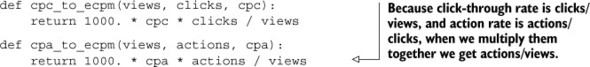
Notice that in our helper functions we used clicks, views, and actions directly instead of the calculated CTR. This lets us keep these values directly in our accounting system, only calculating the eCPM as necessary. Also notice that for our uses, CPC and CPA are similar, the major difference being that for most ads, the number of actions is significantly lower than the number of clicks, but the value per action is typically much larger than the value per click.
Now that we’ve calculated the basic value of an ad, let’s index an ad in preparation for targeting.
Inserting an ad into the index
When targeting an ad, we’ll have a group of optional and required targeting parameters. In order to properly target an ad, our indexing of the ad must reflect the targeting requirements. Since we have two targeting options—location and content—we’ll say that location is required (either on the city, state, or country level), but any matching terms between the ad and the content of the page will be optional and a bonus.[3]
3 If ad copy matches page content, then the ad looks like the page and will be more likely to be clicked on than an ad that doesn’t look like the page content.
We’ll use the same search functions we defined in sections 7.1 and 7.2, with slightly different indexing options. We’ll also assume that you’ve taken my advice from chapter 4 by splitting up your different types of services to different machines (or databases) as necessary, so that your ad-targeting index doesn’t overlap with your other content indexes.
As in section 7.1, we’ll create inverted indexes that use SETs and ZSETs to hold ad IDs. Our SETs will hold the required location targeting, which provides no additional bonus. When we talk about learning from user behavior, we’ll get into how we calculate our per-matched-word bonus, but initially we won’t include any of our terms for targeting bonuses, because we don’t know how much they may contribute to the overall value of the ad. Our ad-indexing function is shown here.
Listing 7.10. A method for indexing an ad that’s targeted on location and ad content
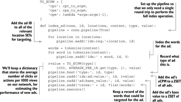
As shown in the listing and described in the annotations, we made three important additions to the listing. The first is that an ad can actually have multiple targeted locations. This is necessary to allow a single ad to be targeted for any one of multiple locations at the same time (like multiple cities, states, or countries).
The second is that we’ll keep a dictionary that holds information about the average number of clicks and actions across the entire system. This lets us come up with a reasonable estimate on the eCPM for CPC and CPA ads before they’ve even been seen in the system.[4]
4 It may seem strange to be estimating an expectation (which is arguably an estimate), but everything about targeting ads is fundamentally predicated on statistics of one kind or another. This is one of those cases where the basics can get us pretty far.
Finally, we’ll also keep a SET of all of the terms that we can optionally target in the ad. I include this information as a precursor to learning about user behavior a little later.
It’s now time to search for and discover ads that match an ad request.
7.3.3. Targeting ads
As described earlier, when we receive a request to target an ad, we’re generally looking to find the highest eCPM ad that matches the viewer’s location. In addition to matching an ad based on a location, we’ll gather and use statistics about how the content of a page matches the content of an ad, and what that can do to affect the ad’s CTR. Using these statistics, content in an ad that matches a web page can result in bonuses that contribute to the calculated eCPM of CPC and CPA ads, which can result in those types of ads being shown more.
Before showing any ads, we won’t have any bonus scoring for any of our web page content. But as we show ads, we’ll learn about what terms in the ads help or hurt the ad’s expected performance, which will allow us to change the relative value of each of the optional targeting terms.
To execute the targeting, we’ll union all of the relevant location SETs to produce an initial group of ads that should be shown to the viewer. Then we’ll parse the content of the page on which the ad will be shown, add any relevant bonuses, and finally calculate a total eCPM for all ads that a viewer could be shown. After we’ve calculated those eCPMs, we’ll fetch the ad ID for the highest eCPM ad, record some statistics about our targeting, and return the ad itself. Our code for targeting an ad looks like this.
Listing 7.11. Ad targeting by location and page content bonuses
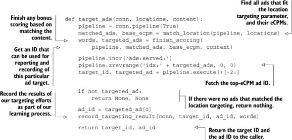
In this first version, we hide away the details of exactly how we’re matching based on location and adding bonuses based on terms so that we can understand the general flow. The only part I didn’t mention earlier is that we’ll also generate a target ID, which is an ID that represents this particular execution of the ad targeting. This ID will allow us to track clicks later, helping us learn about which parts of the ad targeting may have contributed to the overall total clicks.
As mentioned earlier, in order to match based on location, we’ll perform a SET union over the locations (city, state, country) that the viewer is coming from. While we’re here, we’ll also calculate the base eCPM of these ads without any bonuses applied. The code for performing this operation is shown next.
Listing 7.12. A helper function for targeting ads based on location

This code listing does exactly what I said it would do: it finds ads that match the location of the viewer, and it calculates the eCPM of all of those ads without any bonuses based on page content applied. The only thing that may be surprising about this listing is our passing of the funny _execute keyword argument to the zintersect() function, which delays the actual execution of calculating the eCPM of the ad until later. The purpose of waiting until later is to help minimize the number of round trips between our client and Redis.
Calculating targeting bonuses
The interesting part of targeting isn’t the location matching; it’s calculating the bonuses. We’re trying to discover the amount to add to an ad’s eCPM, based on words in the page content that matched words in the ad. We’ll assume that we’ve precalculated a bonus for each word in each ad (as part of the learning phase), stored in ZSETs for each word, with members being ad IDs and scores being what should be added to the eCPM.
These word-based, per-ad eCPM bonuses have values such that the average eCPM of the ad, when shown on a page with that word, is the eCPM bonus from the word plus the known average CPM for the ad. Unfortunately, when more than one word in an ad matches the content of the page, adding all of the eCPM bonuses gives us a total eCPM bonus that probably isn’t close to reality.
We have eCPM bonuses based on word matching for each word that are based on single word matching page content alone, or with any one or a number of other words in the ad. What we really want to find is the weighted average of the eCPMs, where the weight of each word is the number of times the word matched the page content. Unfortunately, we can’t perform the weighted average calculation with Redis ZSETs, because we can’t divide one ZSET by another.
Numerically speaking, the weighted average lies between the geometric average and the arithmetic average, both of which would be reasonable estimates of the combined eCPM. But we can’t calculate either of those averages when the count of matching words varies. The best estimate of the ad’s true eCPM is to find the maximum and minimum bonuses, calculate the average of those two, and use that as the bonus for multiple matching words.
Being mathematically rigorous
Mathematically speaking, our method of averaging the maximum and minimum word bonuses to determine an overall bonus isn’t rigorous. The true mathematical expectation of the eCPM with a collection of matched words is different than what we calculated. We chose to use this mathematically nonrigorous method because it gets us to a reasonable answer (the weighted average of the words is between the minimum and maximum), with relatively little work. If you choose to use this bonus method along with our later learning methods, remember that there are better ways to target ads and to learn from user behavior. I chose this method because it’s easy to write, easy to learn, and easy to improve.
We can calculate the maximum and minimum bonuses by using ZUNIONSTORE with the MAX and MIN aggregates. And we can calculate their average by using them as part of a ZUNIONSTORE operation with an aggregate of SUM, and their weights each being .5. Our function for combining bonus word eCPMs with the base eCPM of the ad can be seen in the next listing.
Listing 7.13. Calculating the eCPM of ads including content match bonuses
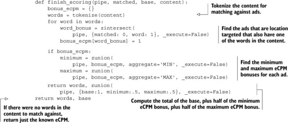
As before, we continue to pass the _execute parameter to delay execution of our various ZINTERSTORE and ZUNIONSTORE operations until after the function returns to the calling target_ads(). One thing that may be confusing is our use of ZINTERSTORE between the location-targeted ads and the bonuses, followed by a final ZUNIONSTORE call. Though we could perform fewer calls by performing a ZUNIONSTORE over all of our bonus ZSETs, followed by a single ZINTERSTORE call at the end (to match location), the majority of ad-targeting calls will perform better by performing many smaller intersections followed by a union.
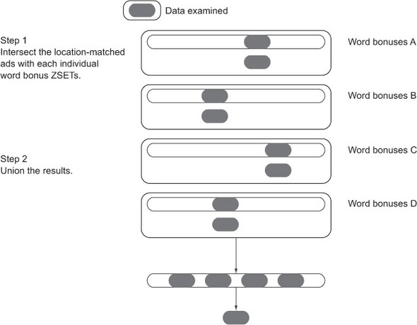
The difference between the two methods is illustrated in figure 7.5, which shows that essentially all of the data in all of the relevant word bonus ZSETs is examined when we union and then intersect. Compare that with figure 7.6, which shows that when we intersect and then union, Redis will examine far less data to produce the same result.
Figure 7.5. The data that’s examined during a union-then-intersect calculation of ad-targeting bonuses includes all ads in the relevant word bonus ZSETs, even ads that don’t meet the location matching requirements.
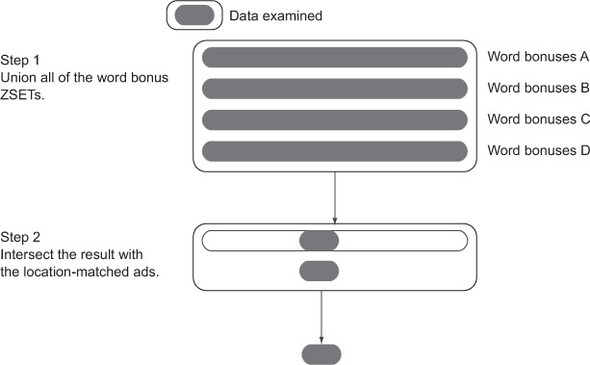
Figure 7.6. The data that’s examined during an intersect-then-union calculation of ad-targeting bonuses only includes those ads that previously matched, which significantly cuts down on the amount of data that Redis will process.
After we have an ad targeted, we’re given a target_id and an ad_id. These IDs would then be used to construct an ad response that includes both pieces of information, in addition to fetching the ad copy, formatting the result, and returning the result to the web page or client that requested it.
If you pay careful attention to the flow of target_ads() through finish_scoring() in listings 7.11 and 7.13, you’ll notice that we don’t make any effort to deal with the case where an ad has zero matched words in the content. In that situation, the eCPM produced will actually be the average eCPM over all calls that returned that ad itself. It’s not difficult to see that this may result in an ad being shown that shouldn’t. Can you alter finish_scoring() to take into consideration ads that don’t match any content?
The only part of our target_ads() function from listing 7.11 that we haven’t defined is record_targeting_result(), which we’ll now examine as part of the learning phase of ad targeting.
7.3.4. Learning from user behavior
As ads are shown to users, we have the opportunity to gain insight into what can cause someone to click on an ad. In the last section, we talked about using words as bonuses to ads that have already matched the required location. In this section, we’ll talk about how we can record information about those words and the ads that were targeted to discover basic patterns about user behavior in order to develop per-word, per-ad-targeting bonuses.
A crucial question you should be asking yourself is “Why are we using words in the web page content to try to find better ads?” The simple reason is that ad placement is all about context. If a web page has content related to the safety of children’s toys, showing an ad for a sports car probably won’t do well. By matching words in the ad with words in the web page content, we get a form of context matching quickly and easily.
One thing to remember during this discussion is that we aren’t trying to be perfect. We aren’t trying to solve the ad-targeting and learning problem completely; we’re trying to build something that will work “pretty well” with simple and straightforward methods. As such, our note about the fact that this isn’t mathematically rigorous still applies.
Recording views
The first step in our learning process is recording the results of our ad targeting with the record_targeting_result() function that we called earlier from listing 7.11. Overall, we’ll record some information about the ad-targeting results, which we’ll later use to help us calculate click-through rates, action rates, and ultimately eCPM bonuses for each word. We’ll record the following:
- Which words were targeted with the given ad
- The total number of times that a given ad has been targeted
- The total number of times that a word in the ad was part of the bonus calculation
To record this information, we’ll store a SET of the words that were targeted and keep counts of the number of times that the ad and words were seen as part of a single ZSET per ad. Our code for recording this information is shown next.
Listing 7.14. A method for recording the result after we’ve targeted an ad
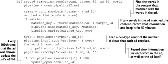
That function does everything we said it would do, and you’ll notice a call to update_cpms(). This update_cpms() function is called every 100th time the ad is returned from a call. This function really is the core of the learning phase—it writes back to our per-word, per-ad-targeting bonus ZSETs.
We’ll get to updating the eCPM of an ad in a moment, but first, let’s see what happens when an ad is clicked.
Recording clicks and actions
As we record views, we’re recording half of the data for calculating CTRs. The other half of the data that we need to record is information about the clicks themselves, or in the case of a cost per action ad, the action. Numerically, this is because our eCPM calculations are based on this formula: (value of a click or action) × (clicks or actions) / views. Without recording clicks and actions, the numerator of our value calculation is 0, so we can’t discover anything useful.
When someone actually clicks on an ad, prior to redirecting them to their final destination, we’ll record the click in the total aggregates for the type of ad, as well as whether the ad got a click and which words matched the clicked ad. We’ll record the same information for actions. Our function for recording clicks is shown next.
Listing 7.15. A method for recording clicks on an ad
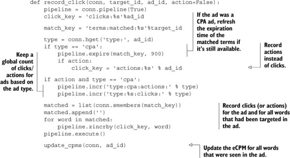
You’ll notice there are a few parts of the recording function that we didn’t mention earlier. In particular, when we receive a click or an action for a CPA ad, we’ll refresh the expiration of the words that were a part of the ad-targeting call. This will let an action following a click count up to 15 minutes after the initial click-through to the destination site happened.
Another change is that we’ll optionally be recording actions in this call for CPA ads; we’ll assume that this function is called with the action parameter set to True in that case.
And finally, we’ll call the update_cpms() function for every click/action because they should happen roughly once every 100–2000 views (or more), so each individual click/action is important relative to a view.
In listing 7.15, we define a record_click() function to add 1 to every word that was targeted as part of an ad that was clicked on. Can you think of a different number to add to a word that may make more sense? Hint: You may want to consider this number to be related to the count of matched words. Can you update finish_scoring() and record_click() to take into consideration this new click/ action value?
To complete our learning process, we only need to define our final update_cpms() function.
Updating eCPMs
We’ve been talking about and using the update_cpms() function for a couple of sections now, and hopefully you already have an idea of what happens inside of it. Regardless, we’ll walk through the different parts of how we’ll update our per-word, per-ad bonus eCPMs, as well as how we’ll update our per-ad eCPMs.
The first part to updating our eCPMs is to know the click-through rate of an ad by itself. Because we’ve recorded both the clicks and views for each ad overall, we have the click-through rate by pulling both of those scores from the relevant ZSETs. By combining that click-through rate with the ad’s actual value, which we fetch from the ad’s base value ZSET, we can calculate the eCPM of the ad over all clicks and views.
The second part to updating our eCPMs is to know the CTR of words that were matched in the ad itself. Again, because we recorded all views and clicks involving the ad, we have that information. And because we have the ad’s base value, we can calculate the eCPM. When we have the word’s eCPM, we can subtract the ad’s eCPM from it to determine the bonus that the word matching contributes. This difference is what’s added to the per-word, per-ad bonus ZSETs.
The same calculation is performed for actions as was performed for clicks, the only difference being that we use the action count ZSETs instead of the click count ZSETs. Our method for updating eCPMs for clicks and actions can be seen in the next listing.
Listing 7.16. A method for updating eCPMs and per-word eCPM bonuses for ads

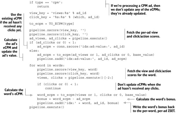
In listing 7.16, we perform a number of round trips to Redis that’s relative to the number of words that were targeted. More specifically, we perform the number of words plus three round trips. In most cases, this should be relatively small (considering that most ads won’t have a lot of content or related keywords). But even so, some of these round trips can be avoided. Can you update the update_cpms() function to perform a total of only three round trips?
In our update_cpms() function, we updated the global per-type click-through and action rates, the per-ad eCPMs, and the per-word, per-ad bonus eCPMs.
With the learning portion of our ad-targeting process now complete, we’ve now built a complete ad-targeting engine from scratch. This engine will learn over time, adapt the ads it returns over time, and more. We can make many possible additions or changes to this engine to make it perform even better, some of which are mentioned in the exercises, and several of which are listed next. These are just starting points for building with Redis:
- Over time, the total number of clicks and views for each ad will stabilize around a particular ratio, and subsequent clicks and views won’t alter that ratio significantly. The real CTR of an ad will vary based on time of day, day of week, and more. Consider degrading an ad’s click/action and view count on a regular basis, as we did in section 2.5 with our rescale_viewed() call. This same concept applies to our global expected CTRs.
- To extend the learning ability beyond just a single count, consider keeping counts over the last day, week, and other time slices. Also consider ways of weighing those time slices differently, depending on their age. Can you think of a method to learn proper weights of different ages of counts?
- All of the big ad networks use second-price auctions in order to charge for a given ad placement. More specifically, rather than charging a fixed rate per click, per thousand views, or per action, you charge a rate that’s relative to the second-highest value ad that was targeted.
- In most ad networks, there’ll be a set of ads that rotate through the highest-value slot for a given set of keywords as each of them runs out of money. These ads are there because their high value and CTR earn the top slot. This means that new ads that don’t have sufficiently high values will never be seen, so the network will never discover them. Rather than picking the highest-eCPM ads 100% of the time, fetch the top 100 ads and choose ads based on the relative values of their eCPMs anywhere from 10%-50% of the time (depending on how you want to balance learning true eCPMs and earning the most money).
- When ads are initially placed into the system, we know little about what to expect in terms of eCPM. We addressed this briefly by using the average CTR of all ads of the same type, but this is moot the moment a single click comes in. Another method mixes the average CTR for a given ad type, along with the seen CTR for the ad based on the number of views that the ad has seen. A simple inverse linear or inverse sigmoid relationship between the two can be used until the ad has had sufficient views (2,000–5,000 views is typically enough to determine a reliable CTR).
- In addition to mixing the average CTR for a given ad type with the CTR of the ad during the learning process, ads that are in the process of reaching an initial 2,000–5,000 views can have their CTR/eCPM artificially boosted. This can ensure sufficient traffic for the system to learn the ads’ actual eCPMs.
- Our method of learning per-word bonuses is similar to Bayesian statistics. We could use real Bayesian statistics, neural networks, association rule learning, clustering, or other techniques to calculate the bonuses. These other methods may offer more mathematically rigorous results, which may result in better CTRs, and ultimately more money earned.
- In our code listings, we recorded views, clicks, and actions as part of the calls that return the ads or handle any sort of redirection. These operations may take a long time to execute, so should be handled after the calls have returned by being executed as an external task, as we discussed in section 6.4.
As you can see from our list, many additions and improvements can and should be made to this platform. But as an initial pass, what we’ve provided can get you started in learning about and building the internet’s next-generation ad-targeting platform.
Now that you’ve learned about how to build an ad-targeting platform, let’s keep going to see how to use search tools to find jobs that candidates are qualified for as part of a job-search tool.
7.4. Job search
If you’re anything like me, at some point in your past you’ve spent time looking through classifieds and online job-search pages, or have used a recruiting agency to try to find work. One of the first things that’s checked (after location) is required experience and/or skills.
In this section, we’ll talk about using Redis SETs and ZSETs to find jobs for which a candidate has all of the required skills. When you’re finished reading this section, you’ll understand another way of thinking about your problem that fits the Redis data model.
As a way of approaching this problem, we’ll say that Fake Garage Startup is branching out in their offerings, trying to pull their individual and group chat customers into using their system to find work. Initially, they’re only offering the ability for users to search for positions in which they’re qualified.
7.4.1. Approaching the problem one job at a time
At first glance, we might consider a straightforward solution to this problem. Start with every job having its own SET, with members being the skills that the job requires. To check whether a candidate has all of the requirements for a given job, we’d add the candidate’s skills to a SET and then perform the SDIFF of the job and the candidate’s skills. If there are no skills in the resulting SDIFF, then the user has all of the qualifications necessary to complete the job. The code for adding a job and checking whether a given set of skills is sufficient for that job looks like this next listing.
Listing 7.17. A potential solution for finding jobs when a candidate meets all requirements
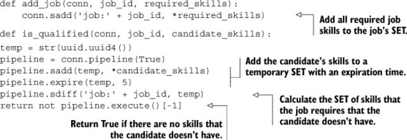
Explaining that again, we’re checking whether a job requires any skills that the candidate doesn’t have. This solution is okay, but it suffers from the fact that to find all of the jobs for a given candidate, we must check each job individually. This won’t scale, but there are solutions that will.
7.4.2. Approaching the problem like search
In section 7.3.3, we used SETs and ZSETs as holders for additive bonuses for optional targeting parameters. If we’re careful, we can do the same thing for groups of required targeting parameters.
Rather than talk about jobs with skills, we need to flip the problem around like we did with the other search problems described in this chapter. We start with one SET per skill, which stores all of the jobs that require that skill. In a required skills ZSET, we store the total number of skills that a job requires. The code that sets up our index looks like the next listing.
Listing 7.18. A function for indexing jobs based on the required skills
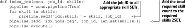
This indexing function should remind you of the text indexing function we used in section 7.1. The only major difference is that we’re providing index_job() with pretokenized skills, and we’re adding a member to a ZSET that keeps a record of the number of skills that each job requires.
To perform a search for jobs that a candidate has all of the skills for, we need to approach the search like we did with the bonuses to ad targeting in section 7.3.3. More specifically, we’ll perform a ZUNIONSTORE operation over skill SETs to calculate a total score for each job. This score represents how many skills the candidate has for each of the jobs.
Because we have a ZSET with the total number of skills required, we can then perform a ZINTERSTORE operation between the candidate’s ZSET and the required skills ZSET with weights -1 and 1, respectively. Any job ID with a score equal to 0 in that final result ZSET is a job that the candidate has all of the required skills for. The code for implementing the search operation is shown in the following listing.
Listing 7.19. Find all jobs that a candidate is qualified for
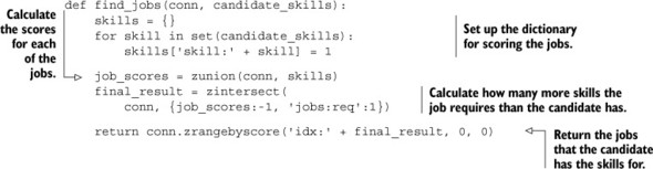
Again, we first find the scores for each job. After we have the scores for each job, we subtract each job score from the total score necessary to match. In that final result, any job with a ZSET score of 0 is a job that the candidate has all of the skills for.
Depending on the number of jobs and searches that are being performed, our job-search system may or may not perform as fast as we need it to, especially with large numbers of jobs or searches. But if we apply sharding techniques that we’ll discuss in chapter 9, we can break the large calculations into smaller pieces and calculate partial results bit by bit. Alternatively, if we first find the SET of jobs in a location to search for jobs, we could perform the same kind of optimization that we performed with ad targeting in section 7.3.3, which could greatly improve job-search performance.
A natural extension to the simple required skills listing is an understanding that skill levels vary from beginner to intermediate, to expert, and beyond. Can you come up with a method using additional SETs to offer the ability, for example, for someone who has as intermediate level in a skill to find jobs that require either beginner or intermediate-level candidates?
Levels of expertise can be useful, but another way to look at the amount of experience someone has is the number of years they’ve used it. Can you build an alternate version that supports handling arbitrary numbers of years of experience?
7.5. Summary
In this chapter, you’ve learned how to perform basic searching using SET operations, and then ordered the results based on either values in HASHes, or potentially composite values with ZSETs. You continued through the steps necessary to build and update information in an ad-targeting network, and you finished with job searching that turned the idea of scoring search results on its head.
Though the problems introduced in this chapter may have been new, one thing that you should’ve gotten used to by now is Redis’s ability to help you solve an unexpectedly wide variety of problems. With the data modeling options available in other databases, you really only have one tool to work with. But with Redis, the five data structures and pub/sub are an entire toolbox for you to work with.
In the next chapter, we’ll continue to use Redis HASHes and ZSETs as building blocks in our construction of a fully functional Twitter clone.