
Chapter 6. Application components in Redis
This chapter covers
- Building two prefix-matching autocomplete methods
- Creating a distributed lock to improve performance
- Developing counting semaphores to control concurrency
- Two task queues for different use cases
- Pull messaging for delayed message delivery
- Handling file distribution
In the last few chapters, we’ve gone through some basic use cases and tools to help build applications in Redis. In this chapter, we’ll get into more useful tools and techniques, working toward building bigger pieces of applications in Redis.
We’ll begin by building autocomplete functions to quickly find users in short and long lists of items. We’ll then take some time to carefully build two different types of locks to reduce data contention, improve performance, prevent data corruption, and reduce wasted work. We’ll construct a delayed task queue, only to augment it later to allow for executing a task at a specific time with the use of the lock we just created. Building on the task queues, we’ll build two different messaging systems to offer point-to-point and broadcast messaging services. We’ll then reuse our earlier IP-address-to-city/-country lookup from chapter 5, and apply it to billions of log entries that are stored and distributed via Redis.
Each component offers usable code and solutions for solving these specific problems in the context of two example companies. But our solutions contain techniques that can be used for other problems, and our specific solutions can be applied to a variety of personal, public, or commercial projects.
To start, let’s look at a fictional web-based game company called Fake Game Company, which currently has more than a million daily players of its games on YouTwitFace, a fictional social network. Later we’ll look at a web/mobile startup called Fake Garage Startup that does mobile and web instant messaging.
6.1. Autocomplete
In the web world, autocomplete is a method that allows us to quickly look up things that we want to find without searching. Generally, it works by taking the letters that we’re typing and finding all words that start with those letters. Some autocomplete tools will even let us type the beginning of a phrase and finish the phrase for us. As an example, autocomplete in Google’s search shows us that Betty White’s SNL appearance is still popular, even years later (which is no surprise—she’s a firecracker). It shows us the URLs we’ve recently visited and want to revisit when we type in the address bar, and it helps us remember login names. All of these functions and more are built to help us access information faster. Some of them, like Google’s search box, are backed by many terabytes of remote information. Others, like our browser history and login boxes, are backed by much smaller local databases. But they all get us what we want with less work.
We’ll build two different types of autocomplete in this section. The first uses lists to remember the most recent 100 contacts that a user has communicated with, trying to minimize memory use. Our second autocomplete offers better performance and scalability for larger lists, but uses more memory per list. They differ in their structure, the methods used, and the time it takes for the operations to complete. Let’s first start with an autocomplete for recent contacts.
6.1.1. Autocomplete for recent contacts
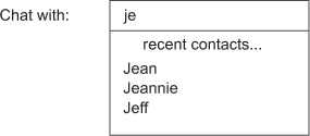
The purpose of this autocomplete is to keep a list of the most recent users that each player has been in contact with. To increase the social aspect of the game and to allow people to quickly find and remember good players, Fake Game Company is looking to create a contact list for their client to remember the most recent 100 people that each user has chatted with. On the client side, when someone is trying to start a chat, they can start typing the name of the person they want to chat with, and autocomplete will show the list of users whose screen names start with the characters they’ve typed. Figure 6.1 shows an example of this kind of autocompletion.
Figure 6.1. A recent contacts autocomplete showing users with names starting with je
Because each of the millions of users on the server will have their own list of their most recent 100 contacts, we need to try to minimize memory use, while still offering the ability to quickly add and remove users from the list. Because Redis LISTs keep the order of items consistent, and because LISTs use minimal memory compared to some other structures, we’ll use them to store our autocomplete lists. Unfortunately, LISTs don’t offer enough functionality to actually perform the autocompletion inside Redis, so we’ll perform the actual autocomplete outside of Redis, but inside of Python. This lets us use Redis to store and update these lists using a minimal amount of memory, leaving the relatively easy filtering to Python.
Generally, three operations need to be performed against Redis in order to deal with the recent contacts autocomplete lists. The first operation is to add or update a contact to make them the most recent user contacted. To perform this operation, we need to perform these steps:
1. Remove the contact from the list if it exists.
2. Add the contact to the beginning of the list.
3. Trim the list if it now has more than 100 items.
We can perform these operations with LREM, LPUSH, and LTRIM, in that order. To make sure that we don’t have any race conditions, we’ll use a MULTI/EXEC transaction around our commands like I described in chapter 3. The complete function is shown in this next listing.
Listing 6.1. The add_update_contact() function
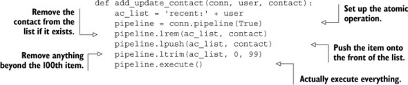
As I mentioned, we removed the user from the LIST (if they were present), pushed the user onto the left side of the LIST; then we trimmed the LIST to ensure that it didn’t grow beyond our limit.
The second operation that we’ll perform is to remove a contact if the user doesn’t want to be able to find them anymore. This is a quick LREM call, which can be seen as follows:
def remove_contact(conn, user, contact):
    conn.lrem('recent:' + user, contact)
The final operation that we need to perform is to fetch the autocomplete list itself to find the matching users. Again, because we’ll perform the actual autocomplete processing in Python, we’ll fetch the whole LIST, and then process it in Python, as shown next.
Listing 6.2. The fetch_autocomplete_list() function
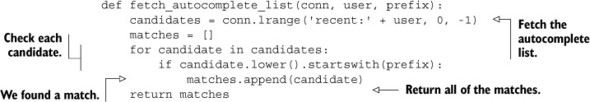
Again, we fetch the entire autocomplete LIST, filter it by whether the name starts with the necessary prefix, and return the results. This particular operation is simple enough that we could even push it off to the client if we find that our server is spending too much time computing it, only requiring a refetch on update.
This autocomplete will work fine for our specific example. It won’t work as well if the lists grow significantly larger, because to remove an item takes time proportional to the length of the list. But because we were concerned about space, and have explicitly limited our lists to 100 users, it’ll be fast enough. If you find yourself in need of much larger most- or least-recently-used lists, you can use ZSETs with timestamps instead.
6.1.2. Address book autocomplete
In the previous example, Redis was used primarily to keep track of the contact list, not to actually perform the autocomplete. This is okay for short lists, but for longer lists, fetching thousands or millions of items to find just a handful would be a waste. Instead, for autocomplete lists with many items, we must find matches inside Redis.
Going back to Fake Game Company, the recent contacts chat autocomplete is one of the most-used social features of our game. Our number-two feature, in-game mailing, has been gaining momentum. To keep the momentum going, we’ll add an autocomplete for mailing. But in our game, we only allow users to send mail to other users that are in the same in-game social group as they are, which we call a guild. This helps to prevent abusive and unsolicited messages between users.
Guilds can grow to thousands of members, so we can’t use our old LIST-based autocomplete method. But because we only need one autocomplete list per guild, we can use more space per member. To minimize the amount of data to be transferred to clients who are autocompleting, we’ll perform the autocomplete prefix calculation inside Redis using ZSETs.
To store each autocomplete list will be different than other ZSET uses that you’ve seen before. Mostly, we’ll use ZSETs for their ability to quickly tell us whether an item is in the ZSET, what position (or index) a member occupies, and to quickly pull ranges of items from anywhere inside the ZSET. What makes this use different is that all of our scores will be zero. By setting our scores to zero, we use a secondary feature of ZSETs: ZSETs sort by member names when scores are equal. When all scores are zero, all members are sorted based on the binary ordering of the strings. In order to actually perform the autocomplete, we’ll insert lowercased contact names. Conveniently enough, we’ve only ever allowed users to have letters in their names, so we don’t need to worry about numbers or symbols.
What do we do? Let’s start by thinking of names as a sorted sequence of strings like abc, abca, abcb, ... abd. If we’re looking for words with a prefix of abc, we’re really looking for strings that are after abbz... and before abd. If we knew the rank of the first item that is before abbz... and the last item after abd, we could perform a ZRANGE call to fetch items between them. But, because we don’t know whether either of those items are there, we’re stuck. To become unstuck, all we really need to do is to insert items that we know are after abbz... and before abd, find their ranks, make our ZRANGE call, and then remove our start and end members.
The good news is that finding an item that’s before abd but still after all valid names with a prefix of abc is easy: we concatenate a { (left curly brace) character onto the end of our prefix, giving us abc{. Why {? Because it’s the next character in ASCII after z. To find the start of our range for abc, we could also concatenate { to abb, getting abb{, but what if our prefix was aba instead of abc? How do we find a character before a? We take a hint from our use of the curly brace, and note that the character that precedes a in ASCII is ` (back quote). So if our prefix is aba, our start member will be ab`, and our end member will be aba{.
Putting it all together, we’ll find the predecessor of our prefix by replacing the last character of our prefix with the character that came right before it. We’ll find the successor of our prefix by concatenating a curly brace. To prevent any issues with two prefix searches happening at the same time, we’ll concatenate a curly brace onto our prefix (for post-filtering out endpoint items if necessary). A function that will generate these types of ranges can be seen next.
Listing 6.3. The find_prefix_range() function
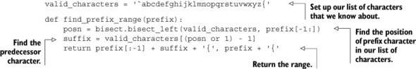
I know, it can be surprising to have spent so many paragraphs describing what we’re going to do, only to end up with just a few lines that actually implement it. But if we look at what we’re doing, we’re just finding the last character in the prefix in our presorted sequence of characters (using the bisect module), and then looking up the character that came just before it.
Character sets and internationalization
This method of finding the preceding and following characters in ASCII works really well for languages with characters that only use characters a-z. But when confronted with characters that aren’t in this range, you’ll find a few new challenges.
First, you’ll have to find a method that turns all of your characters into bytes; three common encodings include UTF-8, UTF-16, and UTF-32 (big-endian and little-endian variants of UTF-16 and UTF-32 are used, but only big-endian versions work in this situation). Second, you’ll need to find the range of characters that you intend to support, ensuring that your chosen encoding leaves at least one character before your supported range and one character after your selected range in the encoded version. Third, you need to use these characters to replace the back quote character ` and the left curly brace character { in our example.
Thankfully, our algorithm doesn’t care about the native sort order of the characters, only the encodings. So you can pick UTF-8 or big-endian UTF-16 or UTF-32, use a null to replace the back quote, and use the maximum value that your encoding and language supports to replace the left curly brace. (Some language bindings are somewhat limited, allowing only up to Unicode code point U+ffff for UTF-16 and Unicode code point U+2ffff for UTF-32.)
After we have the range of values that we’re looking for, we need to insert our ending points into the ZSET, find the rank of those newly added items, pull some number of items between them (we’ll fetch at most 10 to avoid overwhelming the user), and then remove our added items. To ensure that we’re not adding and removing the same items, as would be the case if two members of the same guild were trying to message the same user, we’ll also concatenate a 128-bit randomly generated UUID to our start and end members. To make sure that the ZSET isn’t being changed when we try to find and fetch our ranges, we’ll use WATCH with MULTI and EXEC after we’ve inserted our endpoints. The full autocomplete function is shown here.
Listing 6.4. The autocomplete_on_prefix() function
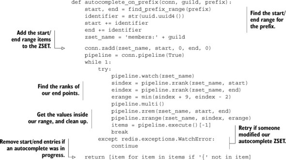
Most of this function is bookkeeping and setup. The first part is just getting our start and ending points, followed by adding them to the guild’s autocomplete ZSET. When we have everything in the ZSET, we WATCH the ZSET to ensure that we discover if someone has changed it, fetch the ranks of the start and end points in the ZSET, fetch items between the endpoints, and clean up after ourselves.
To add and remove members from a guild is straightforward: we only need to ZADD and ZREM the user from the guild’s ZSET. Both of these functions are shown here.
Listing 6.5. The join_guild() and leave_guild() functions
def join_guild(conn, guild, user):
    conn.zadd('members:' + guild, user, 0)

def leave_guild(conn, guild, user):
    conn.zrem('members:' + guild, user)
Joining or leaving a guild, at least when it comes to autocomplete, is straightforward. We only need to add or remove names from the ZSET.
This method of adding items to a ZSET to create a range—fetching items in the range and then removing those added items—can be useful. Here we use it for autocomplete, but this technique can also be used for arbitrary sorted indexes. In chapter 7, we’ll talk about a technique for improving these kinds of operations for a few different types of range queries, which removes the need to add and remove items at the endpoints. We’ll wait to talk about the other method, because it only works on some types of data, whereas this method works on range queries over any type of data.
When we added our endpoints to the ZSET, we needed to be careful about other users trying to autocomplete at the same time, which is why we use the WATCH command. As our load increases, we may need to retry our operations often, which can be wasteful. The next section talks about a way to avoid retries, improve performance, and sometimes simplify our code by reducing and/or replacing WATCH with locks.
6.2. Distributed locking
Generally, when you “lock” data, you first acquire the lock, giving you exclusive access to the data. You then perform your operations. Finally, you release the lock to others. This sequence of acquire, operate, release is pretty well known in the context of shared-memory data structures being accessed by threads. In the context of Redis, we’ve been using WATCH as a replacement for a lock, and we call it optimistic locking, because rather than actually preventing others from modifying the data, we’re notified if someone else changes the data before we do it ourselves.
With distributed locking, we have the same sort of acquire, operate, release operations, but instead of having a lock that’s only known by threads within the same process, or processes on the same machine, we use a lock that different Redis clients on different machines can acquire and release. When and whether to use locks or WATCH will depend on a given application; some applications don’t need locks to operate correctly, some only require locks for parts, and some require locks at every step.
One reason why we spend so much time building locks with Redis instead of using operating system–level locks, language-level locks, and so forth, is a matter of scope. Clients want to have exclusive access to data stored on Redis, so clients need to have access to a lock defined in a scope that all clients can see—Redis. Redis does have a basic sort of lock already available as part of the command set (SETNX), which we use, but it’s not full-featured and doesn’t offer advanced functionality that users would expect of a distributed lock.
Throughout this section, we’ll talk about how an overloaded WATCHed key can cause performance issues, and build a lock piece by piece until we can replace WATCH for some situations.
6.2.1. Why locks are important
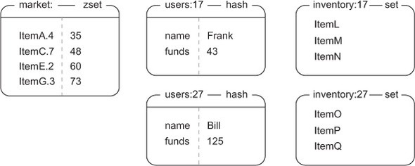
In the first version of our autocomplete, we added and removed items from a LIST. We did so by wrapping our multiple calls with a MULTI/EXEC pair. Looking all the way back to section 4.6, we first introduced WATCH/MULTI/EXEC transactions in the context of an in-game item marketplace. If you remember, the market is structured as a single ZSET, with members being an object and owner ID concatenated, along with the item price as the score. Each user has their own HASH, with columns for user name, currently available funds, and other associated information. Figure 6.2 shows an example of the marketplace, user inventories, and user information.
Figure 6.2. The structure of our marketplace from section 4.6. There are four items in the market on the left—ItemA, ItemC, ItemE, and ItemG—with prices 35, 48, 60, and 73, and seller IDs of 4, 7, 2, and 3, respectively. In the middle we have two users, Frank and Bill, and their current funds, with their inventories on the right.
You remember that to add an item to the marketplace, we WATCH the seller’s inventory to make sure the item is still available, add the item to the market ZSET, and remove it from the user’s inventory. The core of our earlier list_item() function from section 4.4.2 is shown next.
Listing 6.6. The list_item() function from section 4.4.2
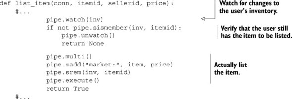
The short comments in this code just hide a lot of the setup and WATCH/MULTI/EXEC handling that hide the core of what we’re doing, which is why I omitted it here. If you feel like you need to see that code again, feel free to jump back to section 4.4.2 to refresh your memory.
Now, to review our purchasing of an item, we WATCH the market and the buyer’s HASH. After fetching the buyer’s total funds and the price of the item, we verify that the buyer has enough money. If the buyer has enough money, we transfer money between the accounts, add the item to the buyer’s inventory, and remove the item from the market. If the buyer doesn’t have enough money, we cancel the transaction. If a WATCH error is caused by someone else writing to the market ZSET or the buyer HASH changing, we retry. The following listing shows the core of our earlier purchase_item() function from section 4.4.3.
Listing 6.7. The purchase_item() function from section 4.4.3
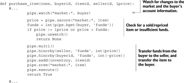
As before, we omit the setup and WATCH/MULTI/EXEC handling to focus on the core of what we’re doing.
To see the necessity of locks at scale, let’s take a moment to simulate the marketplace in a few different loaded scenarios. We’ll have three different runs: one listing and one buying process, then five listing processes and one buying process, and finally five listing and five buying processes. Table 6.1 shows the result of running this simulation.
Table 6.1. Performance of a heavily loaded marketplace over 60 seconds
|
Listed items |
Bought items |
Purchase retries |
Average wait per purchase |
|
|---|---|---|---|---|
| 1 lister, 1 buyer | 145,000 | 27,000 | 80,000 | 14ms |
| 5 listers, 1 buyer | 331,000 | <200 | 50,000 | 150ms |
| 5 listers, 5 buyers | 206,000 | <600 | 161,000 | 498ms |
As our overloaded system pushes its limits, we go from roughly a 3-to-1 ratio of retries per completed sale with one listing and buying process, all the way up to 250 retries for every completed sale. As a result, the latency to complete a sale increases from under 10 milliseconds in the moderately loaded system, all the way up to nearly 500 milliseconds in the overloaded system. This is a perfect example of why WATCH/MULTI/EXEC transactions sometimes don’t scale at load, and it’s caused by the fact that while trying to complete a transaction, we fail and have to retry over and over. Keeping our data correct is important, but so is actually getting work done. To get past this limitation and actually start performing sales at scale, we must make sure that we only list or sell one item in the marketplace at any one time. We do this by using a lock.
6.2.2. Simple locks
In our first simple version of a lock, we’ll take note of a few different potential failure scenarios. When we actually start building the lock, we won’t handle all of the failures right away. We’ll instead try to get the basic acquire, operate, and release process working right. After we have that working and have demonstrated how using locks can actually improve performance, we’ll address any failure scenarios that we haven’t already addressed.
While using a lock, sometimes clients can fail to release a lock for one reason or another. To protect against failure where our clients may crash and leave a lock in the acquired state, we’ll eventually add a timeout, which causes the lock to be released automatically if the process that has the lock doesn’t finish within the given time.
Many users of Redis already know about locks, locking, and lock timeouts. But sadly, many implementations of locks in Redis are only mostly correct. The problem with mostly correct locks is that they’ll fail in ways that we don’t expect, precisely when we don’t expect them to fail. Here are some situations that can lead to incorrect behavior, and in what ways the behavior is incorrect:
- A process acquired a lock, operated on data, but took too long, and the lock was automatically released. The process doesn’t know that it lost the lock, or may even release the lock that some other process has since acquired.
- A process acquired a lock for an operation that takes a long time and crashed. Other processes that want the lock don’t know what process had the lock, so can’t detect that the process failed, and waste time waiting for the lock to be released.
- One process had a lock, but it timed out. Other processes try to acquire the lock simultaneously, and multiple processes are able to get the lock.
- Because of a combination of the first and third scenarios, many processes now hold the lock and all believe that they are the only holders.
Even if each of these problems had a one-in-a-million chance of occurring, because Redis can perform 100,000 operations per second on recent hardware (and up to 225,000 operations per second on high-end hardware), those problems can come up when under heavy load,[1] so it’s important to get locking right.
1 Having tested a few available Redis lock implementations that include support for timeouts, I was able to induce lock duplication on at least half of the lock implementations with just five clients acquiring and releasing the same lock over 10 seconds.
6.2.3. Building a lock in Redis
Building a mostly correct lock in Redis is easy. Building a completely correct lock in Redis isn’t much more difficult, but requires being extra careful about the operations we use to build it. In this first version, we’re not going to handle the case where a lock times out, or the case where the holder of the lock crashes and doesn’t release the lock. Don’t worry; we’ll get to those cases in the next section, but for now, let’s just get basic locking correct.
The first part of making sure that no other code can run is to acquire the lock. The natural building block to use for acquiring a lock is the SETNX command, which will only set a value if the key doesn’t already exist. We’ll set the value to be a unique identifier to ensure that no other process can get the lock, and the unique identifier we’ll use is a 128-bit randomly generated UUID.
If we fail to acquire the lock initially, we’ll retry until we acquire the lock, or until a specified timeout has passed, whichever comes first, as shown here.
Listing 6.8. The acquire_lock() function
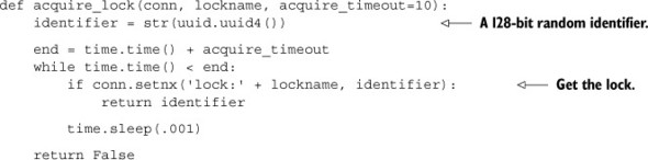
As described, we’ll attempt to acquire the lock by using SETNX to set the value of the lock’s key only if it doesn’t already exist. On failure, we’ll continue to attempt this until we’ve run out of time (which defaults to 10 seconds).
Now that we have the lock, we can perform our buying or selling without WATCH errors getting in our way. We’ll acquire the lock and, just like before, check the price of the item, make sure that the buyer has enough money, and if so, transfer the money and item. When completed, we release the lock. The code for this can be seen next.
Listing 6.9. The purchase_item_with_lock() function
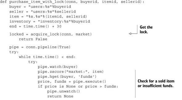
Looking through the code listing, it almost seems like we’re locking the operation. But don’t be fooled—we’re locking the market data, and the lock must exist while we’re operating on the data, which is why it surrounds the code performing the operation.
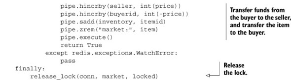
To release the lock, we have to be at least as careful as when acquiring the lock. Between the time when we acquired the lock and when we’re trying to release it, someone may have done bad things to the lock. To release the lock, we need to WATCH the lock key, and then check to make sure that the value is still the same as what we set it to before we delete it. This also prevents us from releasing a lock multiple times. The release_lock() function is shown next.
Listing 6.10. The release_lock() function
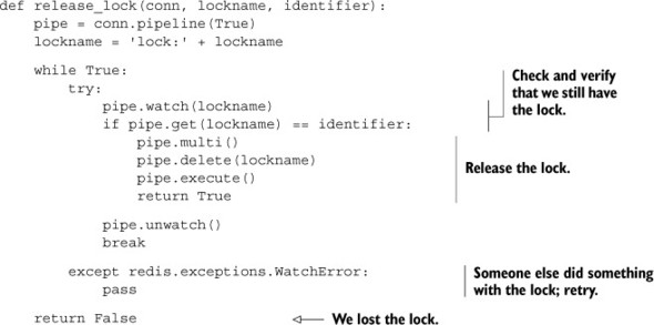
We take many of the same steps to ensure that our lock hasn’t changed as we did with our money transfer in the first place. But if you think about our release lock function for long enough, you’ll (reasonably) come to the conclusion that, except in very rare situations, we don’t need to repeatedly loop. But the next version of the acquire lock function that supports timeouts, if accidentally mixed with earlier versions (also unlikely, but anything is possible with code), could cause the release lock transaction to fail and could leave the lock in the acquired state for longer than necessary. So, just to be extra careful, and to guarantee correctness in as many situations as possible, we’ll err on the side of caution.
After we’ve wrapped our calls with locks, we can perform the same simulation of buying and selling as we did before. In table 6.2, we have new rows that use the lock-based buying and selling code, which are shown below our earlier rows.
Table 6.2. Performance of locking over 60 seconds
|
Listed items |
Bought items |
Purchase retries |
Average wait per purchase |
|
|---|---|---|---|---|
| 1 lister, 1 buyer, no lock | 145,000 | 27,000 | 80,000 | 14ms |
| 1 lister, 1 buyer, with lock | 51,000 | 50,000 | 0 | 1ms |
| 5 listers, 1 buyer, no lock | 331,000 | <200 | 50,000 | 150ms |
| 5 listers, 1 buyer, with lock | 68,000 | 13,000 | <10 | 5ms |
| 5 listers, 5 buyers, no lock | 206,000 | <600 | 161,000 | 498ms |
| 5 listers, 5 buyers, with lock | 21,000 | 20,500 | 0 | 14ms |
Though we generally have lower total number of items that finished being listed, we never retry, and our number of listed items compared to our number of purchased items is close to the ratio of number of listers to buyers. At this point, we’re running at the limit of contention between the different listing and buying processes.
6.2.4. Fine-grained locking
When we introduced locks and locking, we only worried about providing the same type of locking granularity as the available WATCH command—on the level of the market key that we were updating. But because we’re constructing locks manually, and we’re less concerned about the market in its entirety than we are with whether an item is still in the market, we can actually lock on a finer level of detail. If we replace the market-level lock with one specific to the item to be bought or sold, we can reduce lock contention and increase performance.
Let’s look at the results in table 6.3, which is the same simulation as produced table 6.2, only with locks over just the items being listed or sold individually, and not over the entire market.
Table 6.3. Performance of fine-grained locking over 60 seconds
|
Listed items |
Bought items |
Purchase retries |
Average wait per purchase |
|
|---|---|---|---|---|
| 1 lister, 1 buyer, no lock | 145,000 | 27,000 | 80,000 | 14ms |
| 1 lister, 1 buyer, with lock | 51,000 | 50,000 | 0 | 1ms |
| 1 lister, 1 buyer, with fine-grained lock | 113,000 | 110,000 | 0 | <1ms |
| 5 listers, 1 buyer, no lock | 331,000 | <200 | 50,000 | 150ms |
| 5 listers, 1 buyer, with lock | 68,000 | 13,000 | <10 | 5ms |
| 5 listers, 1 buyer, with fine-grained lock | 192,000 | 36,000 | 0 | <2ms |
| 5 listers, 5 buyers, no lock | 206,000 | <600 | 161,000 | 498ms |
| 5 listers, 5 buyers, with lock | 21,000 | 20,500 | 0 | 14ms |
| 5 listers, 5 buyers, with fine-grained lock | 116,000 | 111,000 | 0 | <3ms |
With fine-grained locking, we’re performing 220,000–230,000 listing and buying operations regardless of the number of listing and buying processes. We have no retries, and even under a full load, we’re seeing less than 3 milliseconds of latency. Our listed-to-sold ratio is again almost exactly the same as our ratio of listing-to-buying processes. Even better, we never get into a situation like we did without locks where there’s so much contention that latencies shoot through the roof and items are rarely sold.
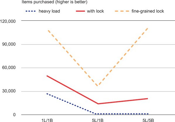
Let’s take a moment to look at our data as a few graphs so that we can see the relative scales. In figure 6.3, we can see that both locking methods result in much higher numbers of items being purchased over all relative loads than the WATCH-based method.
Figure 6.3. Items purchased completed in 60 seconds. This graph has an overall V shape because the system is overloaded, so when we have five listing processes to only one buying process (shown as 5L/1B in the middle samples), the ratio of listed items to bought items is roughly the same ratio, 5 to 1.
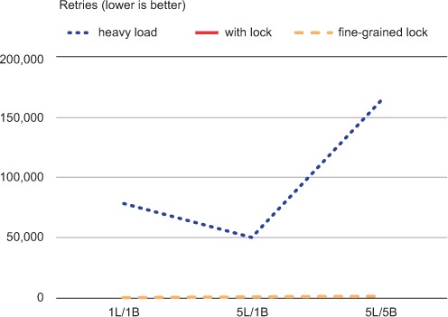
Looking at figure 6.4, we can see that the WATCH-based method has to perform many thousands of expensive retries in order to complete what few sales are completed.
Figure 6.4. The number of retries when trying to purchase an item in 60 seconds. There are no retries for either types of locks, so we can’t see the line for “with lock” because it’s hidden behind the line for fine-grained locks.
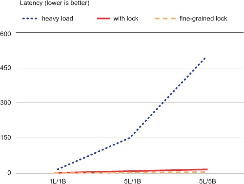
And in figure 6.5, we can see that because of the WATCH contention, which caused the huge number of retries and the low number of purchase completions, latency without using a lock went up significantly.
Figure 6.5. Average latency for a purchase; times are in milliseconds. The maximum latency for either kind of lock is under 14ms, which is why both locking methods are difficult to see and hugging the bottom—our overloaded system without a lock has an average latency of nearly 500ms.
What these simulations and these charts show overall is that when under heavy load, using a lock can reduce retries, reduce latency, improve performance, and be tuned at the granularity that we need.
Our simulation is limited. One major case that it doesn’t simulate is where many more buyers are unable to buy items because they’re waiting for others. It also doesn’t simulate an effect known as dogpiling, when, as transactions take longer to complete, more transactions are overlapping and trying to complete. That will increase the time it takes to complete an individual transaction, and subsequently increase the chances for a time-limited transaction to fail. This will substantially increase the failure and retry rates for all transactions, but it’s especially harmful in the WATCH-based version of our market buying and selling.
The choice to use a lock over an entire structure, or over just a small portion of a structure, can be easy. In our case, the critical data that we were watching was a small piece of the whole (one item in a marketplace), so locking that small piece made sense. There are situations where it’s not just one small piece, or when it may make sense to lock multiple parts of structures. That’s where the decision to choose locks over small pieces of data or an entire structure gets difficult; the use of multiple small locks can lead to deadlocks, which can prevent any work from being performed at all.
6.2.5. Locks with timeouts
As mentioned before, our lock doesn’t handle cases where a lock holder crashes without releasing the lock, or when a lock holder fails and holds the lock forever. To handle the crash/failure cases, we add a timeout to the lock.
In order to give our lock a timeout, we’ll use EXPIRE to have Redis time it out automatically. The natural place to put the EXPIRE is immediately after the lock is acquired, and we’ll do that. But if our client happens to crash (and the worst place for it to crash for us is between SETNX and EXPIRE), we still want the lock to eventually time out. To handle that situation, any time a client fails to get the lock, the client will check the expiration on the lock, and if it’s not set, set it. Because clients are going to be checking and setting timeouts if they fail to get a lock, the lock will always have a timeout, and will eventually expire, letting other clients get a timed-out lock.
What if multiple clients set expiration times simultaneously? They’ll run at essentially the same time, so expiration will be set for the same time.
Adding expiration to our earlier acquire_lock() function gets us the updated acquire_lock_with_timeout() function shown here.
Listing 6.11. The acquire_lock_with_timeout() function
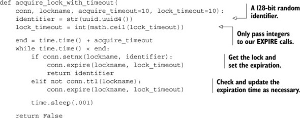
This new acquire_lock_with_timeout() handling timeouts. It ensures that locks expire as necessary, and that they won’t be stolen from clients that rightfully have them. Even better, we were smart with our release lock function earlier, which still works.
Note
As of Redis 2.6.12, the SET command added options to support a combination of SETNX and SETEX functionality, which makes our lock acquire function trivial. We still need the complicated release lock to be correct.
In section 6.1.2 when we built the address book autocomplete using a ZSET, we went through a bit of trouble to create start and end entries to add to the ZSET in order to fetch a range. We also postprocessed our data to remove entries with curly braces ({}), because other autocomplete operations could be going on at the same time. And because other operations could be going on at the same time, we used WATCH so that we could retry. Each of those pieces added complexity to our functions, which could’ve been simplified if we’d used a lock instead.
In other databases, locking is a basic operation that’s supported and performed automatically. As I mentioned earlier, using WATCH, MULTI, and EXEC is a way of having an optimistic lock—we aren’t actually locking data, but we’re notified and our changes are canceled if someone else modifies it before we do. By adding explicit locking on the client, we get a few benefits (better performance, a more familiar programming concept, easier-to-use API, and so on), but we need to remember that Redis itself doesn’t respect our locks. It’s up to us to consistently use our locks in addition to or instead of WATCH, MULTI, and EXEC to keep our data consistent and correct.
Now that we’ve built a lock with timeouts, let’s look at another kind of lock called a counting semaphore. It isn’t used in as many places as a regular lock, but when we need to give multiple clients access to the same information at the same time, it’s the perfect tool for the job.
6.3. Counting semaphores
A counting semaphore is a type of lock that allows you to limit the number of processes that can concurrently access a resource to some fixed number. You can think of the lock that we just created as being a counting semaphore with a limit of 1. Generally, counting semaphores are used to limit the amount of resources that can be used at one time.
Like other types of locks, counting semaphores need to be acquired and released. First, we acquire the semaphore, then we perform our operation, and then we release it. But where we’d typically wait for a lock if it wasn’t available, it’s common to fail immediately if a semaphore isn’t immediately available. For example, let’s say that we wanted to allow for five processes to acquire the semaphore. If a sixth process tried to acquire it, we’d want that call to fail early and report that the resource is busy.
We’ll move through this section similarly to how we went through distributed locking in section 6.2. We’ll build a counting semaphore piece by piece until we have one that’s complete and correct.
Let’s look at an example with Fake Game Company. With the success of its marketplace continuously growing, Fake Game Company has had requests from users wanting to access information about the marketplace from outside the game so that they can buy and sell items without being logged into the game. The API to perform these operations has already been written, but it’s our job to construct a mechanism that limits each account from accessing the marketplace from more than five processes at a time.
After we’ve built our counting semaphore, we make sure to wrap incoming API calls with a proper acquire_semaphore() and release_semaphore() pair.
6.3.1. Building a basic counting semaphore
When building a counting semaphore, we run into many of the same concerns we had with other types of locking. We must decide who got the lock, how to handle processes that crashed with the lock, and how to handle timeouts. If we don’t care about timeouts, or handling the case where semaphore holders can crash without releasing semaphores, we could build semaphores fairly conveniently in a few different ways. Unfortunately, those methods don’t lead us to anything useful in the long term, so I’ll describe one method that we’ll incrementally improve to offer a full range of functionality.
In almost every case where we want to deal with timeouts in Redis, we’ll generally look to one of two different methods. Either we’ll use EXPIRE like we did with our standard locks, or we’ll use ZSETs. In this case, we want to use ZSETs, because that allows us to keep information about multiple semaphore holders in a single structure.
More specifically, for each process that attempts to acquire the semaphore, we’ll generate a unique identifier. This identifier will be the member of a ZSET. For the score, we’ll use the timestamp for when the process attempted to acquire the semaphore. Our semaphore ZSET will look something like figure 6.6.
Figure 6.6. Basic semaphore ZSET
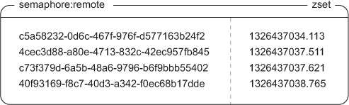
When a process wants to attempt to acquire a semaphore, it first generates an identifier, and then the process adds the identifier to the ZSET using the current timestamp as the score. After adding the identifier, the process then checks for its identifier’s rank. If the rank returned is lower than the total allowed count (Redis uses 0-indexing on rank), then the caller has acquired the semaphore. Otherwise, the caller doesn’t have the semaphore and must delete its identifier from the ZSET. To handle timeouts, before adding our identifier to the ZSET, we first clear out any entries that have timestamps that are older than our timeout number value. The code to acquire the semaphore can be seen next.
Listing 6.12. The acquire_semaphore() function
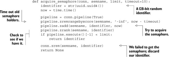
Our code proceeds as I’ve already described: generating the identifier, cleaning out any timed-out semaphores, adding its identifier to the ZSET, and checking its rank. Not too surprising.
Releasing the semaphore is easy: we remove the identifier from the ZSET, as can be seen in the next listing.
Listing 6.13. The release_semaphore() function
This basic semaphore works well—it’s simple, and it’s very fast. But relying on every process having access to the same system time in order to get the semaphore can cause problems if we have multiple hosts. This isn’t a huge problem for our specific use case, but if we had two systems A and B, where A ran even 10 milliseconds faster than B, then if A got the last semaphore, and B tried to get a semaphore within 10 milliseconds, B would actually “steal” A’s semaphore without A knowing it.
Any time we have a lock or a semaphore where such a slight difference in the system clock can drastically affect who can get the lock, the lock or semaphore is considered unfair. Unfair locks and semaphores can cause clients that should’ve gotten the lock or semaphore to never get it, and this is something that we’ll fix in the next section.
6.3.2. Fair semaphores
Because we can’t assume that all system clocks are exactly the same on all systems, our earlier basic counting semaphore will have issues where clients on systems with slower system clocks can steal the semaphore from clients on systems with faster clocks. Any time there’s this kind of sensitivity, locking itself becomes unfair. We want to reduce the effect of incorrect system times on acquiring the semaphore to the point where as long as systems are within 1 second, system time doesn’t cause semaphore theft or early semaphore expiration.
In order to minimize problems with inconsistent system times, we’ll add a counter and a second ZSET. The counter creates a steadily increasing timer-like mechanism that ensures that whoever incremented the counter first should be the one to get the semaphore. We then enforce our requirement that clients that want the semaphore who get the counter first also get the semaphore by using an “owner” ZSET with the counter-produced value as the score, checking our identifier’s rank in the new ZSET to determine which client got the semaphore. The new owner ZSET appears in figure 6.7.
Figure 6.7. Fair semaphore owner ZSET
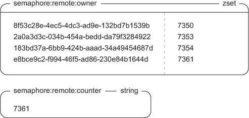
We continue to handle timeouts the same way as our basic semaphore, by removing entries from the system time ZSET. We propagate those timeouts to the new owner ZSET by the use of ZINTERSTORE and the WEIGHTS argument.
Bringing it all together in listing 6.14, we first time out an entry by removing old entries from the timeout ZSET and then intersect the timeout ZSET with the owner ZSET, saving to and overwriting the owner ZSET. We then increment the counter and add our counter value to the owner ZSET, while at the same time adding our current system time to the timeout ZSET. Finally, we check whether our rank in the owner ZSET is low enough, and if so, we have a semaphore. If not, we remove our entries from the owner and timeout ZSETs.
Listing 6.14. The acquire_fair_semaphore() function
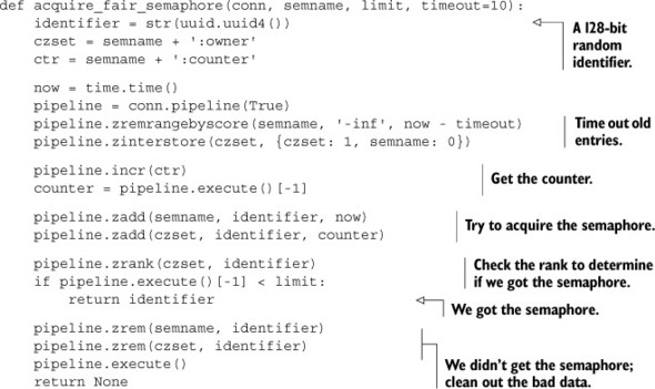
This function has a few different pieces. We first clean up timed-out semaphores, updating the owner ZSET and fetching the next counter ID for this item. After we’ve added our time to the timeout ZSET and our counter value to the owner ZSET, we’re ready to check to see whether our rank is low enough.
Fair semaphores on 32-bit platforms
On 32-bit Redis platforms, integer counters are limited to 231 - 1, the standard signed integer limit. An overflow situation could occur on heavily used semaphores roughly once every 2 hours in the worst case. Though there are a variety of workarounds, the simplest is to switch to a 64-bit platform for any machine using any counter-based ID.
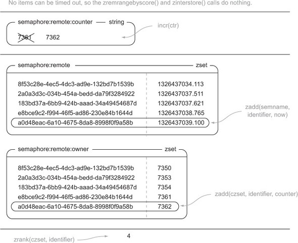
Let’s look at figure 6.8, which shows the sequence of operations that are performed when process ID 8372 wants to acquire the semaphore at time 1326437039.100 when there’s a limit of 5.
Figure 6.8. Call sequence for acquire_fair_semaphore()
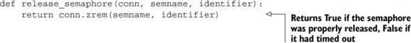
Releasing the semaphore is almost as easy as before, only now we remove our identifier from both the owner and timeout ZSETs, as can be seen in this next listing.
Listing 6.15. The release_fair_semaphore() function
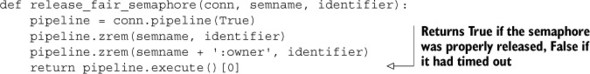
If we wanted to be lazy, in most situations we could just remove our semaphore identifier from the timeout ZSET; one of our steps in the acquire sequence is to refresh the owner ZSET to remove identifiers that are no longer in the timeout ZSET. But by only removing our identifier from the timeout ZSET, there’s a chance (rare, but possible) that we removed the entry, but the acquire_fair_semaphore() was between the part where it updated the owner ZSET and when it added its own identifiers to the timeout and owner ZSETs. If so, this could prevent it from acquiring the semaphore when it should’ve been able to. To ensure correct behavior in as many situations as possible, we’ll stick to removing the identifier from both ZSETs.
Now we have a semaphore that doesn’t require that all hosts have the same system time, though system times do need to be within 1 or 2 seconds in order to ensure that semaphores don’t time out too early, too late, or not at all.
6.3.3. Refreshing semaphores
As the API for the marketplace was being completed, it was decided that there should be a method for users to stream all item listings as they happen, along with a stream for all purchases that actually occur. The semaphore method that we created only supports a timeout of 10 seconds, primarily to deal with timeouts and possible bugs on our side of things. But users of the streaming portion of the API will want to keep connected for much longer than 10 seconds, so we need a method for refreshing the semaphore so that it doesn’t time out.
Because we already separated the timeout ZSET from the owner ZSET, we can actually refresh timeouts quickly by updating our time in the timeout ZSET, shown in the following listing.
Listing 6.16. The refresh_fair_semaphore() function
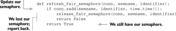
As long as we haven’t already timed out, we’ll be able to refresh the semaphore. If we were timed out in the past, we’ll go ahead and let the semaphore be lost and report to the caller that it was lost. When using a semaphore that may be refreshed, we need to be careful to refresh often enough to not lose the semaphore.
Now that we have the ability to acquire, release, and refresh a fair semaphore, it’s time to deal with our final race condition.
6.3.4. Preventing race conditions
As you saw when building locks in section 6.2, dealing with race conditions that cause retries or data corruption can be difficult. In this case, the semaphores that we created have race conditions that we alluded to earlier, which can cause incorrect operation.
We can see the problem in the following example. If we have two processes A and B that are trying to get one remaining semaphore, and A increments the counter first but B adds its identifier to the ZSETs and checks its identifier’s rank first, then B will get the semaphore. When A then adds its identifier and checks its rank, it’ll “steal” the semaphore from B, but B won’t know until it tries to release or renew the semaphore.
When we were using the system clock as a way of getting a lock, the likelihood of this kind of a race condition coming up and resulting in more than the desired number of semaphore owners was related to the difference in system times—the greater the difference, the greater the likelihood. After introducing the counter with the owner ZSET, this problem became less likely (just by virtue of removing the system clock as a variable), but because we have multiple round trips, it’s still possible.
To fully handle all possible race conditions for semaphores in Redis, we need to reuse the earlier distributed lock with timeouts that we built in section 6.2.5. We need to use our earlier lock to help build a correct counting semaphore. Overall, to acquire the semaphore, we’ll first try to acquire the lock for the semaphore with a short timeout. If we got the lock, we then perform our normal semaphore acquire operations with the counter, owner ZSET, and the system time ZSET. If we failed to acquire the lock, then we say that we also failed to acquire the semaphore. The code for performing this operation is shown next.
Listing 6.17. The acquire_semaphore_with_lock() function
def acquire_semaphore_with_lock(conn, semname, limit, timeout=10):
    identifier = acquire_lock(conn, semname, acquire_timeout=.01)
    if identifier:
        try:
            return acquire_fair_semaphore(conn, semname, limit, timeout)
        finally:
            release_lock(conn, semname, identifier)
I know, it can be disappointing to come so far only to end up needing to use a lock at the end. But that’s the thing with Redis: there are usually a few ways to solve the same or a similar problem, each with different trade-offs. Here are some of the trade-offs for the different counting semaphores that we’ve built:
- If you’re happy with using the system clock, never need to refresh the semaphore, and are okay with occasionally going over the limit, then you can use the first semaphore we created.
- If you can only really trust system clocks to be within 1 or 2 seconds, but are still okay with occasionally going over your semaphore limit, then you can use the second one.
- If you need your semaphores to be correct every single time, then you can use a lock to guarantee correctness.
Now that we’ve used our lock from section 6.2 to help us fix the race condition, we have varying options for how strict we want to be with our semaphore limits. Generally it’s a good idea to stick with the last, strictest version. Not only is the last semaphore actually correct, but whatever time we may save using a simpler semaphore, we could lose by using too many resources.
In this section, we used semaphores to limit the number of API calls that can be running at any one time. Another common use case is to limit concurrent requests to databases to reduce individual query times and to prevent dogpiling like we talked about at the end of section 6.2.4. One other common situation is when we’re trying to download many web pages from a server, but their robots.txt says that we can only make (for example) three requests at a time. If we have many clients downloading web pages, we can use a semaphore to ensure that we aren’t pushing a given server too hard.
As we finish with building locks and semaphores to help improve performance for concurrent execution, it’s now time to talk about using them in more situations. In the next section, we’ll build two different types of task queues for delayed and concurrent task execution.
6.4. Task queues
When handling requests from web clients, sometimes operations take more time to execute than we want to spend immediately. We can defer those operations by putting information about our task to be performed inside a queue, which we process later. This method of deferring work to some task processor is called a task queue. Right now there are many different pieces of software designed specifically for task queues (ActiveMQ, RabbitMQ, Gearman, Amazon SQS, and others), but there are also ad hoc methods of creating task queues in situations where queues aren’t expected. If you’ve ever had a cron job that scans a database table for accounts that have been modified/checked before or after a specific date/time, and you perform some operation based on the results of that query, you’ve already created a task queue.
In this section we’ll talk about two different types of task queues. Our first queue will be built to execute tasks as quickly as possible in the order that they were inserted. Our second type of queue will have the ability to schedule tasks to execute at some specific time in the future.
6.4.1. First-in, first-out queues
In the world of queues beyond task queues, normally a few different kinds of queues are discussed—first-in, first-out (FIFO), last-in first-out (LIFO), and priority queues. We’ll look first at a first-in, first-out queue, because it offers the most reasonable semantics for our first pass at a queue, can be implemented easily, and is fast. Later, we’ll talk about adding a method for coarse-grained priorities, and even later, time-based queues.
Let’s again look back to an example from Fake Game Company. To encourage users to play the game when they don’t normally do so, Fake Game Company has decided to add the option for users to opt-in to emails about marketplace sales that have completed or that have timed out. Because outgoing email is one of those internet services that can have very high latencies and can fail, we need to keep the act of sending emails for completed or timed-out sales out of the typical code flow for those operations. To do this, we’ll use a task queue to keep a record of people who need to be emailed and why, and will implement a worker process that can be run in parallel to send multiple emails at a time if outgoing mail servers become slow.
The queue that we’ll write only needs to send emails out in a first-come, first-served manner, and will log both successes and failures. As we talked about in chapters 3 and 5, Redis LISTs let us push and pop items from both ends with RPUSH/LPUSH and RPOP/LPOP. For our email queue, we’ll push emails to send onto the right end of the queue with RPUSH, and pop them off the left end of the queue with LPOP. (We do this because it makes sense visually for readers of left-to-right languages.) Because our worker processes are only going to be performing this emailing operation, we’ll use the blocking version of our list pop, BLPOP, with a timeout of 30 seconds. We’ll only handle item-sold messages in this version for the sake of simplicity, but adding support for sending timeout emails is also easy.
Our queue will simply be a list of JSON-encoded blobs of data, which will look like figure 6.9.
Figure 6.9. A first-in, first-out queue using a LIST
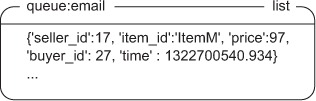
To add an item to the queue, we’ll get all of the necessary information together, serialize it with JSON, and RPUSH the result onto our email queue. As in previous chapters, we use JSON because it’s human readable and because there are fast libraries for translation to/from JSON in most languages. The function that pushes an email onto the item-sold email task queue appears in the next listing.
Listing 6.18. The send_sold_email_via_queue() function
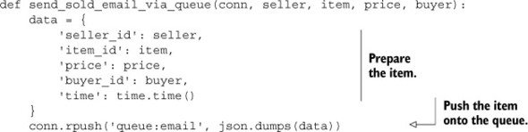
Adding a message to a LIST queue shouldn’t be surprising.
Sending emails from the queue is easy. We use BLPOP to pull items from the email queue, prepare the email, and finally send it. The next listing shows our function for doing so.
Listing 6.19. The process_sold_email_queue() function
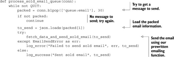
Similarly, actually sending the email after pulling the message from the queue is also not surprising. But what about executing more than one type of task?
Multiple executable tasks
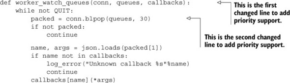
Because Redis only gives a single caller a popped item, we can be sure that none of the emails are duplicated and sent twice. Because we only put email messages to send in the queue, our worker process was simple. Having a single queue for each type of message is not uncommon for some situations, but for others, having a single queue able to handle many different types of tasks can be much more convenient. Take the worker process in listing 6.20: it watches the provided queue and dispatches the JSON-encoded function call to one of a set of known registered callbacks. The item to be executed will be of the form ['FUNCTION_NAME', [ARG1, ARG2, ...]].
Listing 6.20. The worker_watch_queue() function
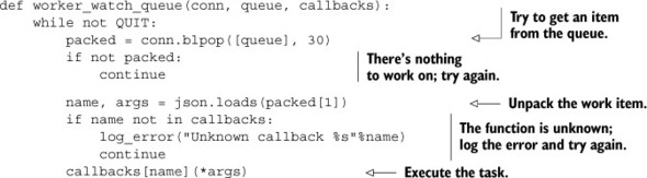
With this generic worker process, our email sender could be written as a callback and passed with other callbacks.
Task priorities
Sometimes when working with queues, it’s necessary to prioritize certain operations before others. In our case, maybe we want to send emails about sales that completed before we send emails about sales that expired. Or maybe we want to send password reset emails before we send out emails for an upcoming special event. Remember the BLPOP/BRPOP commands—we can provide multiple LISTs in which to pop an item from; the first LIST to have any items in it will have its first item popped (or last if we’re using BRPOP).
Let’s say that we want to have three priority levels: high, medium, and low. High-priority items should be executed if they’re available. If there are no high-priority items, then items in the medium-priority level should be executed. If there are neither high- nor medium-priority items, then items in the low-priority level should be executed. Looking at our earlier code, we can change two lines to make that possible in the updated listing.
Listing 6.21. The worker_watch_queues() function
By using multiple queues, priorities can be implemented easily. There are situations where multiple queues are used as a way of separating different queue items (announcement emails, notification emails, and so forth) without any desire to be “fair.” In such situations, it can make sense to reorder the queue list occasionally to be more fair to all of the queues, especially in the case where one queue can grow quickly relative to the other queues.
If you’re using Ruby, you can use an open source package called Resque that was put out by the programmers at GitHub. It uses Redis for Ruby-based queues using lists, which is similar to what we’ve talked about here. Resque offers many additional features over the 11-line function that we provided here, so if you’re using Ruby, you should check it out. Regardless, there are many more options for queues in Redis, and you should keep reading.
6.4.2. Delayed tasks
With list-based queues, we can handle single-call per queue, multiple callbacks per queue, and we can handle simple priorities. But sometimes, we need a bit more. Fake Game Company has decided that they’re going to add a new feature in their game: delayed selling. Rather than putting an item up for sale now, players can tell the game to put an item up for sale in the future. It’s our job to change or replace our task queue with something that can offer this feature.
There are a few different ways that we could potentially add delays to our queue items. Here are the three most straightforward ones:
- We could include an execution time as part of queue items, and if a worker process sees an item with an execution time later than now, it can wait for a brief period and then re-enqueue the item.
- The worker process could have a local waiting list for any items it has seen that need to be executed in the future, and every time it makes a pass through its while loop, it could check that list for any outstanding items that need to be executed.
- Normally when we talk about times, we usually start talking about ZSETs. What if, for any item we wanted to execute in the future, we added it to a ZSET instead of a LIST, with its score being the time when we want it to execute? We then have a process that checks for items that should be executed now, and if there are any, the process removes it from the ZSET, adding it to the proper LIST queue.
We can’t wait/re-enqueue items as described in the first, because that’ll waste the worker process’s time. We also can’t create a local waiting list as described in the second option, because if the worker process crashes for an unrelated reason, we lose any pending work items it knew about. We’ll instead use a secondary ZSET as described in the third option, because it’s simple, straightforward, and we can use a lock from section 6.2 to ensure that the move is safe.
Each delayed item in the ZSET queue will be a JSON-encoded list of four items: a unique identifier, the queue where the item should be inserted, the name of the callback to call, and the arguments to pass to the callback. We include the unique identifier in order to differentiate all calls easily, and to allow us to add possible reporting features later if we so choose. The score of the item will be the time when the item should be executed. If the item can be executed immediately, we’ll insert the item into the list queue instead. For our unique identifier, we’ll again use a 128-bit randomly generated UUID. The code to create an (optionally) delayed task can be seen next.
Listing 6.22. The execute_later() function
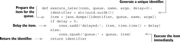
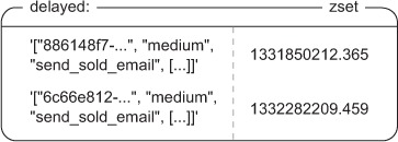
When the queue item is to be executed without delay, we continue to use the old list-based queue. But if we need to delay the item, we add the item to the delayed ZSET. An example of the delayed queue emails to be sent can be seen in figure 6.10.
Figure 6.10. A delayed task queue using a ZSET
Unfortunately, there isn’t a convenient method in Redis to block on ZSETs until a score is lower than the current Unix timestamp, so we need to manually poll. Because delayed items are only going into a single queue, we can just fetch the first item with the score. If there’s no item, or if the item still needs to wait, we’ll wait a brief period and try again. If there is an item, we’ll acquire a lock based on the identifier in the item (a fine-grained lock), remove the item from the ZSET, and add the item to the proper queue. By moving items into queues instead of executing them directly, we only need to have one or two of these running at any time (instead of as many as we have workers), so our polling overhead is kept low. The code for polling our delayed queue is in the following listing.
Listing 6.23. The poll_queue() function
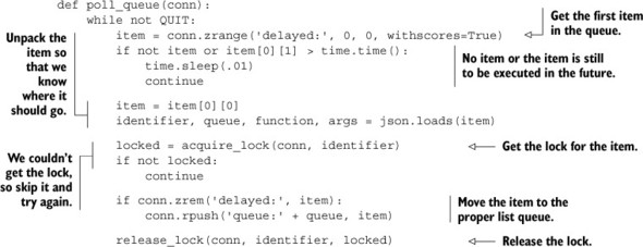
As is clear from listing 6.23, because ZSETs don’t have a blocking pop mechanism like LISTs do, we need to loop and retry fetching items from the queue. This can increase load on the network and on the processors performing the work, but because we’re only using one or two of these pollers to move items from the ZSET to the LIST queues, we won’t waste too many resources. If we further wanted to reduce overhead, we could add an adaptive method that increases the sleep time when it hasn’t seen any items in a while, or we could use the time when the next item was scheduled to help determine how long to sleep, capping it at 100 milliseconds to ensure that tasks scheduled only slightly in the future are executed in a timely fashion.
Respecting priorities
In the basic sense, delayed tasks have the same sort of priorities that our first-in, first-out queue had. Because they’ll go back on their original destination queues, they’ll be executed with the same sort of priority. But what if we wanted delayed tasks to execute as soon as possible after their time to execute has come up?
The simplest way to do this is to add some extra queues to make scheduled tasks jump to the front of the queue. If we have our high-, medium-, and low-priority queues, we can also create high-delayed, medium-delayed, and low-delayed queues, which are passed to the worker_watch_queues() function as ["high-delayed", "high", "medium-delayed", "medium", "low-delayed", "low"]. Each of the delayed queues comes just before its nondelayed equivalent.
Some of you may be wondering, “If we’re having them jump to the front of the queue, why not just use LPUSH instead of RPUSH?” Suppose that all of our workers are working on tasks for the medium queue, and will take a few seconds to finish. Suppose also that we have three delayed tasks that are found and LPUSHed onto the front of the medium queue. The first is pushed, then the second, and then the third. But on the medium queue, the third task to be pushed will be executed first, which violates our expectations that things that we want to execute earlier should be executed earlier.
If you use Python and you’re interested in a queue like this, I’ve written a package called RPQueue that offers delayed task execution semantics similar to the preceding code snippets. It does include more functionality, so if you want a queue and are already using Redis, give RPQueue a look at http://github.com/josiahcarlson/rpqueue/.
When we use task queues, sometimes we need our tasks to report back to other parts of our application with some sort of messaging system. In the next section, we’ll talk about creating message queues that can be used to send to a single recipient, or to communicate between many senders and receivers.
6.5. Pull messaging
When sending and receiving messages between two or more clients, there are two common ways of looking at how the messages are delivered. One method, called push messaging, causes the sender to spend some time making sure that all of the recipients of the message receive it. Redis has built-in commands for handling push messaging called PUBLISH and SUBSCRIBE, whose drawbacks and use we discussed in chapter 3.[2] The second method, called pull messaging, requires that the recipients of the message fetch the messages instead. Usually, messages will wait in a sort of mailbox for the recipient to fetch them.
2 Briefly, these drawbacks are that the client must be connected at all times to receive messages, disconnections can cause the client to lose messages, and older versions of Redis could become unusable, crash, or be killed if there was a slow subscriber.
Though push messaging can be useful, we run into problems when clients can’t stay connected all the time for one reason or another. To address this limitation, we’ll write two different pull messaging methods that can be used as a replacement for PUBLISH/SUBSCRIBE.
We’ll first start with single-recipient messaging, since it shares much in common with our first-in, first-out queues. Later in this section, we’ll move to a method where we can have multiple recipients of a message. With multiple recipients, we can replace Redis PUBLISH and SUBSCRIBE when we need our messages to get to all recipients, even if they were disconnected.
6.5.1. Single-recipient publish/subscribe replacement
One common pattern that we find with Redis is that we have clients of one kind or another (server processes, users in a chat, and so on) that listen or wait for messages on their own channel. They’re the only ones that receive those messages. Many programmers will end up using Redis PUBLISH and SUBSCRIBE commands to send messages and wait for messages, respectively. But if we need to receive messages, even in the face of connection issues, PUBLISH and SUBSCRIBE don’t help us much.
Breaking from our game company focus, Fake Garage Startup wants to release a mobile messaging application. This application will connect to their web servers to send and receive SMS/MMS-like messages (basically a text or picture messaging replacement). The web server will be handling authentication and communication with the Redis back end, and Redis will be handling the message routing/storage.
Each message will only be received by a single client, which greatly simplifies our problem. To handle messages in this way, we use a single LIST for each mobile client. Senders cause messages to be placed in the recipient’s LIST, and any time the recipient’s client makes a request, it fetches the most recent messages. With HTTP 1.1’s ability to pipeline requests, or with more modern web socket support, our mobile client can either make a request for all waiting messages (if any), can make requests one at a time, or can fetch 10 and use LTRIM to remove the first 10 items.
Because you already know how to push and pop items from lists from earlier sections, most recently from our first-in, first-out queues from section 6.4.1, we’ll skip including code to send messages, but an example incoming message queue for user jack451 is illustrated in figure 6.11.
Figure 6.11. jack451 has some messages from Jill and his mother waiting for him.
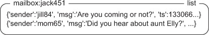
With LISTs, senders can also be notified if the recipient hasn’t been connecting recently, hasn’t received their previous messages, or maybe has too many pending messages; all by checking the messages in the recipient’s LIST. If the system were limited by a recipient needing to be connected all the time, as is the case with PUBLISH/SUBSCRIBE, messages would get lost, clients wouldn’t know if their message got through, and slow clients could result in outgoing buffers growing potentially without limit (in older versions of Redis) or getting disconnected (in newer versions of Redis).
With single-recipient messaging out of the way, it’s time to talk about replacing PUBLISH and SUBSCRIBE when we want to have multiple listeners to a given channel.
6.5.2. Multiple-recipient publish/subscribe replacement
Single-recipient messaging is useful, but it doesn’t get us far in replacing the PUBLISH and SUBSCRIBE commands when we have multiple recipients. To do that, we need to turn our problem around. In many ways, Redis PUBLISH/SUBSCRIBE is like group chat where whether someone’s connected determines whether they’re in the group chat. We want to remove that “need to be connected all the time” requirement, and we’ll implement it in the context of chatting.
Let’s look at Fake Garage Startup’s next problem. After quickly implementing their user-to-user messaging system, Fake Garage Startup realized that replacing SMS is good, but they’ve had many requests to add group chat functionality. Like before, their clients may connect or disconnect at any time, so we can’t use the built-in PUBLISH/SUBSCRIBE method.
Each new group chat will have a set of original recipients of the group messages, and users can join or leave the group if they want. Information about what users are in the chat will be stored as a ZSET with members being the usernames of the recipients, and values being the highest message ID the user has received in the chat. Which chats an individual user is a part of will also be stored as a ZSET, with members being the groups that the user is a part of, and scores being the highest message ID that the user has received in that chat. Information about some users and chats can be seen in figure 6.12.
Figure 6.12. Some example chat and user data. The chat ZSETs show users and the maximum IDs of messages in that chat that they’ve seen. The seen ZSETs list chat IDs per user, again with the maximum message ID in the given chat that they’ve seen.
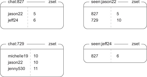
As you can see, user jason22 has seen five of six chat messages sent in chat:827, in which jason22 and jeff24 are participating.
Creating a chat session
The content of chat sessions themselves will be stored in ZSETs, with messages as members and message IDs as scores. To create and start a chat, we’ll increment a global counter to get a new chat ID. We’ll then create a ZSET with all of the users that we want to include with seen IDs being 0, and add the group to each user’s group list ZSET. Finally, we’ll send the initial message to the users by placing the message in the chat ZSET. The code to create a chat is shown here.
Listing 6.24. The create_chat() function
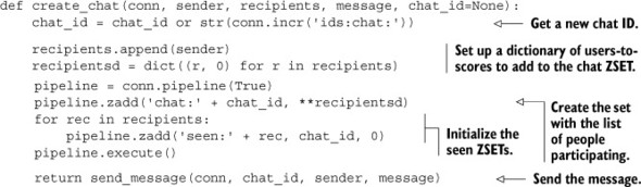
About the only thing that may be surprising is our use of what’s called a generator expression from within a call to the dict() object constructor. This shortcut lets us quickly construct a dictionary that maps users to an initially 0-valued score, which ZADD can accept in a single call.
Generator expressions and dictionary construction
Python dictionaries can be easily constructed by passing a sequence of pairs of values. The first item in the pair becomes the key; the second item becomes the value. Listing 6.24 shows some code that looks odd, where we actually generate the sequence to be passed to the dictionary in-line. This type of sequence generation is known as a generator expression, which you can read more about at http://mng.bz/TTKb.
Sending messages
To send a message, we must get a new message ID, and then add the message to the chat’s messages ZSET. Unfortunately, there’s a race condition in sending messages, but it’s easily handled with the use of a lock from section 6.2. Our function for sending a message using a lock is shown next.
Listing 6.25. The send_message() function
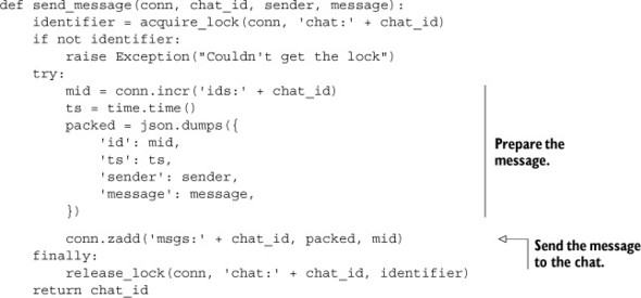
Most of the work involved in sending a chat message is preparing the information to be sent itself; actually sending the message involves adding it to a ZSET. We use locking around the packed message construction and addition to the ZSET for the same reasons that we needed a lock for our counting semaphore earlier. Generally, when we use a value from Redis in the construction of another value we need to add to Redis, we’ll either need to use a WATCH/MULTI/EXEC transaction or a lock to remove race conditions. We use a lock here for the same performance reasons that we developed it in the first place.
Now that we’ve created the chat and sent the initial message, users need to find out information about the chats they’re a part of and how many messages are pending, and they need to actually receive the messages.
Fetching messages
To fetch all pending messages for a user, we need to fetch group IDs and message IDs seen from the user’s ZSET with ZRANGE. When we have the group IDs and the messages that the user has seen, we can perform ZRANGEBYSCORE operations on all of the message ZSETs. After we’ve fetched the messages for the chat, we update the seen ZSET with the proper ID and the user entry in the group ZSET, and we go ahead and clean out any messages from the group chat that have been received by everyone in the chat, as shown in the following listing.
Listing 6.26. The fetch_pending_messages() function
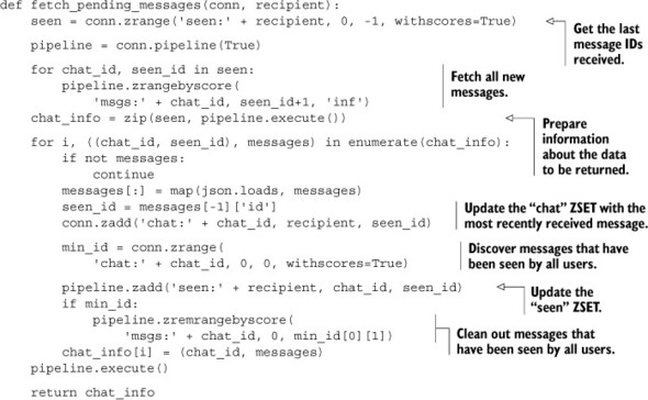
Fetching pending messages is primarily a matter of iterating through all of the chats for the user, pulling the messages, and cleaning up messages that have been seen by all users in a chat.
Joining and leaving the chat
We’ve sent and fetched messages from group chats; all that remains is joining and leaving the group chat. To join a group chat, we fetch the most recent message ID for the chat, and we add the chat information to the user’s seen ZSET with the score being the most recent message ID. We also add the user to the group’s member list, again with the score being the most recent message ID. See the next listing for the code for joining a group.
Listing 6.27. The join_chat() function
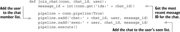
Joining a chat only requires adding the proper references to the user to the chat, and the chat to the user’s seen ZSET.
To remove a user from the group chat, we remove the user ID from the chat ZSET, and we remove the chat from the user’s seen ZSET. If there are no more users in the chat ZSET, we delete the messages ZSET and the message ID counter. If there are users remaining, we’ll again take a pass and clean out any old messages that have been seen by all users. The function to leave a chat is shown in the following listing.
Listing 6.28. The leave_chat() function
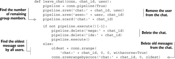
Cleaning up after a user when they leave a chat isn’t that difficult, but requires taking care of a lot of little details to ensure that we don’t end up leaking a ZSET or ID somewhere.
We’ve now finished creating a complete multiple-recipient pull messaging system in Redis. Though we’re looking at it in terms of chat, this same method can be used to replace the PUBLISH/SUBSCRIBE functions when you want your recipients to be able to receive messages that were sent while they were disconnected. With a bit of work, we could replace the ZSET with a LIST, and we could move our lock use from sending a message to old message cleanup. We used a ZSET instead, because it saves us from having to fetch the current message ID for every chat. Also, by making the sender do more work (locking around sending a message), the multiple recipients are saved from having to request more data and to lock during cleanup, which will improve performance overall.
We now have a multiple-recipient messaging system to replace PUBLISH and SUBSCRIBE for group chat. In the next section, we’ll use it as a way of sending information about key names available in Redis.
6.6. Distributing files with Redis
When building distributed software and systems, it’s common to need to copy, distribute, or process data files on more than one machine. There are a few different common ways of doing this with existing tools. If we have a single server that will always have files to be distributed, it’s not uncommon to use NFS or Samba to mount a path or drive. If we have files whose contents change little by little, it’s also common to use a piece of software called Rsync to minimize the amount of data to be transferred between systems. Occasionally, when many copies need to be distributed among machines, a protocol called BitTorrent can be used to reduce the load on the server by partially distributing files to multiple machines, which then share their pieces among themselves.
Unfortunately, all of these methods have a significant setup cost and value that’s somewhat relative. NFS and Samba can work well, but both can have significant issues when network connections aren’t perfect (or even if they are perfect), due to the way both of these technologies are typically integrated with operating systems. Rsync is designed to handle intermittent connection issues, since each file or set of files can be partially transferred and resumed, but it suffers from needing to download complete files before processing can start, and requires interfacing our software with Rsync in order to fetch the files (which may or may not be a problem). And though BitTorrent is an amazing technology, it only really helps if we’re running into limits sending from our server, or if our network is underutilized. It also relies on interfacing our software with a BitTorrent client that may not be available on all platforms, and which may not have a convenient method to fetch files.
Each of the three methods described also require setup and maintenance of users, permissions, and/or servers. Because we already have Redis installed, running, and available, we’ll use Redis to distribute files instead. By using Redis, we bypass issues that some other software has: our client handles connection issues well, we can fetch the data directly with our clients, and we can start processing data immediately (no need to wait for an entire file).
6.6.1. Aggregating users by location
Let’s take a moment and look back at an earlier problem that we solved for Fake Game Company. With the ability to discover where users are accessing the game from thanks to our IP-to-city lookup in chapter 5, Fake Game Company has found itself needing to reparse many gigabytes of log files. They’re looking to aggregate user visitation patterns over time in a few different dimensions: per country, per region, per city, and more. Because we need this to be run in real time over new data, we’ve already implemented callbacks to perform the aggregate operations.
As you may remember from chapter 5, Fake Game Company has been around for about 2 years. They have roughly 1,000,000 users per day, but they have roughly 10 events per user per day. That gives us right around 7.3 billion log lines to process. If we were to use one of the earlier methods, we’d copy the log files to various machines that need to process the data, and then go about processing the log files. This works, but then we need to copy the data, potentially delaying processing, and using storage space on every machine that processes the data, which later needs to be cleaned up.
In this particular case, instead of copying files around, we could write a one-time map-reduce[3] process to handle all of this data. But because map-reduces are designed to not share memory between items to be processed (each item is usually one log line), we can end up taking more time with map-reduce than if we spent some time writing it by hand to share memory. More specifically, if we load our IP-to-city lookup table into memory in Python (which we’d only want to do if we had a lot of processing to do, and we do), we can perform about 200k IP-to-city ID lookups per second, which is faster than we could expect a single Redis instance to respond to the same queries. Also, to scale with map-reduce, we’d have to run at least a few instances of Redis to keep up with the map-reduces.
3 MapReduce (or Map/Reduce) is a type of distributed computation popularized by Google, which can offer high performance and simplicity for some problems.
With the three standard methods of handling this already discounted (NFS/Samba, copying files, map-reduce), let’s look at some other practical pieces that we’ll need to solve to actually perform all of our lookups.
Aggregating data locally
In order to process that many log entries efficiently, we’ll need to locally cache aggregates before updating Redis in order to minimize round trips. Why? If we have roughly 10 million log lines to process for each day, then that’s roughly 10 million writes to Redis. If we perform the aggregates locally on a per-country basis for the entire day (being that there are around 300 countries), we can instead write 300 values to Redis. This will significantly reduce the number of round trips between Redis, reducing the number of commands processed, which in turn will reduce the total processing time.
If we don’t do anything intelligent about local caching, and we have 10 aggregates that we want to calculate, we’re looking at around 10 days to process all of the data. But anything on the country or region level can be aggregated completely (for the day) before being sent to Redis. And generally because the top 10% of cities (there are roughly 350,000 cities in our sample dataset) amount for more than 90% of our game’s users, we can also locally cache any city-level aggregates. So by performing local caching of aggregates, we’re not limited by Redis on aggregate throughput.
Assuming that we’ve already cached a copy of our ZSET and HASH table for IP lookups from section 5.3, we only need to worry about aggregating the data. Let’s start with the log lines that contain an IP address, date, time, and the operation that was performed, similar to the following snippet:
173.194.38.137 2011-10-10 13:55:36 achievement-762
Given log lines of that form, let’s aggregate those lines on a daily basis per country. To do this, we’ll receive the line as part of a call and increment the appropriate counter. If the log line is empty, then we’ll say that the day’s worth of data is done, and we should write to Redis. The source code for performing this aggregate is shown next.
Listing 6.29. A locally aggregating callback for a daily country-level aggregate
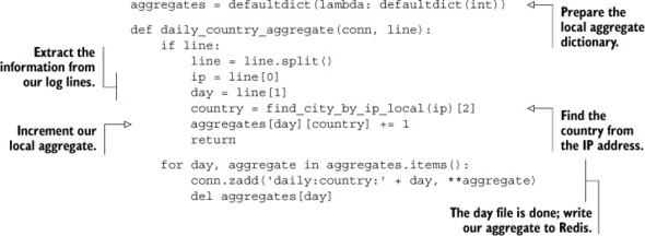
Now that we’ve written and seen one of these aggregate functions, the rest are fairly similar and just as easy to write. Let’s move on to more interesting topics, like how we’re going to send files through Redis.
6.6.2. Sending files
In order to get the log data to our logs processors, we’ll have two different components operating on the data. The first is a script that will be taking the log files and putting them in Redis under named keys, publishing the names of the keys to a chat channel using our group chat method from section 6.5.2, and waiting for notification when they’re complete (to not use more memory than our Redis machine has). It’ll be waiting for a notification that a key with a name similar to the file stored in Redis has a value equal to 10, which is our number of aggregation processes. The function that copies logs and cleans up after itself is shown in the following listing.
Listing 6.30. The copy_logs_to_redis() function
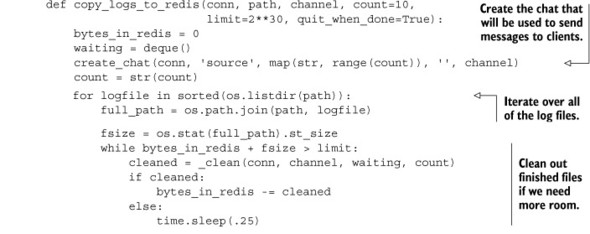
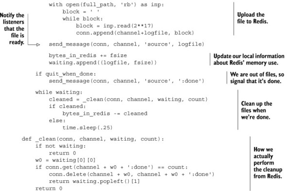
Copying logs to Redis requires a lot of detailed steps, mostly involving being careful to not put too much data into Redis at one time and properly cleaning up after ourselves when a file has been read by all clients. The actual aspect of notifying logs processors that there’s a new file ready is easy, but the setup, sending, and cleanup are pretty detailed.
6.6.3. Receiving files
The second part of the process is a group of functions and generators that will fetch log filenames from the group chat. After receiving each name, it’ll process the log files directly from Redis, and will update the keys that the copy process is waiting on. This will also call our callback on each incoming line, updating our aggregates. The next listing shows the code for the first of these functions.
Listing 6.31. The process_logs_from_redis() function
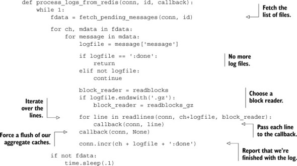
Receiving information about log files is straightforward, though we do defer a lot of the hard work of actually reading the file from Redis to helper functions that generate sequences of log lines. We also need to be careful to notify the file sender by incrementing the counter for the log file; otherwise the file sending process won’t know to clean up finished log files.
6.6.4. Processing files
We’re deferring some of the work of decoding our files to functions that return generators over data. The readlines() function takes the connection, key, and a block-iterating callback. It’ll iterate over blocks of data yielded by the block-iterating callback, discover line breaks, and yield lines. When provided with blocks as in listing 6.32, it finds the last line ending in the block, and then splits the lines up to that last line ending, yielding the lines one by one. When it’s done, it keeps any partial lines to prepend onto the next block. If there’s no more data, it yields the last line by itself. There are other ways of finding line breaks and extracting lines in Python, but the rfind()/split() combination is faster than other methods.
Listing 6.32. The readlines() function
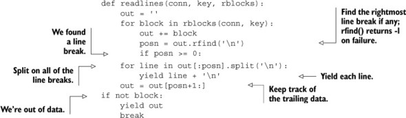
For our higher-level line-generating function, we’re iterating over blocks produced by one of two readers, which allows us to focus on finding line breaks.
Generators with yield
Listing 6.32 offers our first real use of Python generators with the yield statement. Generally, this allows Python to suspend and resume execution of code primarily to allow for easy iteration over sequences or pseudo-sequences of data. For more details on how generators work, you can visit the Python language tutorial with this short URL: http://mng.bz/Z2b1.
Each of the two block-yielding callbacks, readblocks() and readblocks_gz(), will read blocks of data from Redis. The first yields the blocks directly, whereas the other automatically decompresses gzip files. We’ll use this particular layer separation in order to offer the most useful and reusable data reading method possible. The following listing shows the readblocks() generator.
Listing 6.33. The readblocks() generator
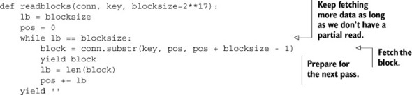
The readblocks() generator is primarily meant to offer an abstraction over our block reading, which allows us to replace it later with other types of readers, like maybe a filesystem reader, a memcached reader, a ZSET reader, or in our case, a block reader that handles gzip files in Redis. The next listing shows the readblocks_gz() generator.
Listing 6.34. The readblocks_gz() generator
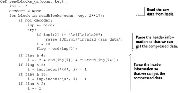
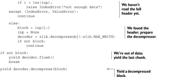
Much of the body of readblocks_gz() is gzip header parsing code, which is unfortunately necessary. For log files (like we’re parsing), gzip can offer a reduction of 2–5 times in storage space requirements, while offering fairly high-speed decompression. Though more modern compression methods are able to compress better (bzip2, lzma/xz, and many others) or faster (lz4, lzop, snappy, QuickLZ, and many others), no other method is as widely available (bzip2 comes close) or has such a useful range of compression ratio and CPU utilization trade-off options.
6.7. Summary
In this chapter we’ve gone through six major topics, but in looking at those topics, we actually solved nine different problems. Whenever possible, we’ve taken steps to borrow ideas and functionality from previous sections to keep building more useful tools, while trying to highlight that many of the techniques that we use in one solution can also be used to solve other problems.
If there’s one concept that you should take away from this entire chapter, it’s that although WATCH is a useful command, is built in, convenient, and so forth, having access to a working distributed lock implementation from section 6.2 can make concurrent Redis programming so much easier. Being able to lock at a finer level of detail than an entire key can reduce contention, and being able to lock around related operations can reduce operation complexity. We saw both performance improvements and operation simplicity in our revisited marketplace example from section 4.6, and in our delayed task queue from section 6.4.2.
If there’s a second concept that you should remember, take to heart, and apply in the future, it’s that with a little work, you can build reusable components with Redis. We reused locks explicitly in counting semaphores, delayed task queues, and in our multiple-recipient pub/sub replacement. And we reused our multiple-recipient pub/sub replacement when we distributed files with Redis.
In the next chapter, we’ll continue with building more advanced tools with Redis, writing code that can be used to back entire applications from document indexing and search with scored indexing and sorting, all the way to an ad targeting system, and a job search system. Going forward, we’ll reuse some of these components in later chapters, so keep an eye out, and remember that it’s not difficult to build reusable components for Redis.