Chapter 10. Scaling Redis

This chapter covers

• Scaling reads
• Scaling writes and memory capacity
• Scaling complex queries

As your use of Redis grows, there may come a time when you’re no longer able to fit all of your data into a single Redis server, or when you need to perform more reads and/or writes than Redis can sustain. When this happens, you have a few options to help you scale Redis to your needs.

In this chapter, we’ll cover techniques to help you to scale your read queries, write queries, total memory available, and techniques for scaling a selection of more complicated queries.

Our first task is addressing those problems where we can store all of the data we need, and we can handle writes without issue, but where we need to perform more read queries in a second than a single Redis server can handle.

10.1. Scaling reads

In chapter 8 we built a social network that offered many of the same features and functionalities of Twitter. One of these features was the ability for users to view their home timeline as well as their profile timeline. When viewing these timelines, we’ll be fetching 30 posts at a time. For a small social network, this wouldn’t be a serious issue, since we could still support anywhere from 3,000–10,000 users fetching timelines every second (if that was all that Redis was doing). But for a larger social network, it wouldn’t be unexpected to need to serve many times that number of timeline fetches every second.

In this section, we’ll discuss the use of read slaves to support scaling read queries beyond what a single Redis server can handle.

Before we get into scaling reads, let’s first review a few opportunities for improving performance before we must resort to using additional servers with slaves to scale our queries:

• If we’re using small structures (as we discussed in chapter 9), first make sure that our max ziplist size isn’t too large to cause performance penalties.
• Remember to use structures that offer good performance for the types of queries we want to perform (don’t treat LISTs like SETs; don’t fetch an entire HASH just to sort on the client—use a ZSET; and so on).
• If we’re sending large objects to Redis for caching, consider compressing the data to reduce network bandwidth for reads and writes (compare lz4, gzip, and bzip2 to determine which offers the best trade-offs for size/performance for our uses).
• Remember to use pipelining (with or without transactions, depending on our requirements) and connection pooling, as we discussed in chapter 4.

When we’re doing everything that we can to ensure that reads and writes are fast, it’s time to address the need to perform more read queries. The simplest method to increase total read throughput available to Redis is to add read-only slave servers. If you remember from chapter 4, we can run additional servers that connect to a master, receive a replica of the master’s data, and be kept up to date in real time (more or less, depending on network bandwidth). By running our read queries against one of several slaves, we can gain additional read query capacity with every new slave.

Remember: Write to the master

When using read slaves, and generally when using slaves at all, you must remember to write to the master Redis server only. By default, attempting to write to a Redis server configured as a slave (even if it’s also a master) will cause that server to reply with an error. We’ll talk about using a configuration option to allow for writes to slave servers in section 10.3.1, but generally you should run with slave writes disabled; writing to slaves is usually an error.

Chapter 4 has all the details on configuring Redis for replication to slave servers, how it works, and some ideas for scaling to many read slaves. Briefly, we can update the Redis configuration file with a line that reads slaveof host port, replacing host and port with the host and port of the master server. We can also configure a slave by running the SLAVEOF host port command against an existing server. Remember: When a slave connects to a master, any data that previously existed on the slave will be discarded. To disconnect a slave from a master to stop it from slaving, we can run SLAVEOF no one.

One of the biggest issues that arises when using multiple Redis slaves to serve data is what happens when a master temporarily or permanently goes down. Remember that when a slave connects, the Redis master initiates a snapshot. If multiple slaves connect before the snapshot completes, they’ll all receive the same snapshot. Though this is great from an efficiency perspective (no need to create multiple snapshots), sending multiple copies of a snapshot at the same time to multiple slaves can use up the majority of the network bandwidth available to the server. This could cause high latency to/from the master, and could cause previously connected slaves to become disconnected.

One method of addressing the slave resync issue is to reduce the total data volume that’ll be sent between the master and its slaves. This can be done by setting up intermediate replication servers to form a type of tree, as can be seen in figure 10.1, which we borrow from chapter 4.

Figure 10.1. An example Redis master/slave replica tree with nine lowest-level slaves and three intermediate replication helper servers

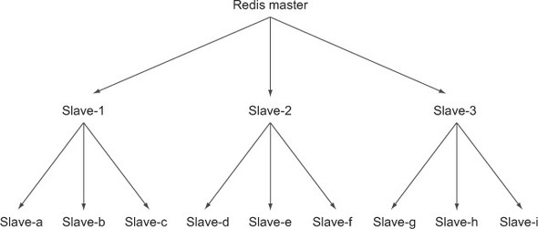
These slave trees will work, and can be necessary if we’re looking to replicate to a different data center (resyncing across a slower WAN link will take resources, which should be pushed off to an intermediate slave instead of running against the root master). But slave trees suffer from having a complex network topology that makes manually or automatically handling failover situations difficult.

An alternative to building slave trees is to use compression across our network links to reduce the volume of data that needs to be transferred. Some users have found that using SSH to tunnel a connection with compression dropped bandwidth use significantly. One company went from using 21 megabits of network bandwidth for replicating to a single slave to about 1.8 megabits (http://mng.bz/2ivv). If you use this method, you’ll want to use a mechanism that automatically reconnects a disconnected SSH connection, of which there are several options to choose from.

Encryption and compression overhead

Generally, encryption overhead for SSH tunnels shouldn’t be a huge burden on your server, since AES-128 can encrypt around 180 megabytes per second on a single core of a 2.6 GHz Intel Core 2 processor, and RC4 can encrypt about 350 megabytes per second on the same machine. Assuming that you have a gigabit network link, roughly one moderately powerful core can max out the connection with encryption. Compression is where you may run into issues, because SSH compression defaults to gzip. At compression level 1 (you can configure SSH to use a specific compression level; check the man pages for SSH), our trusty 2.6 GHz processor can compress roughly 24–52 megabytes per second of a few different types of Redis dumps (the initial sync), and 60–80 megabytes per second of a few different types of append-only files (streaming replication). Remember that, though higher compression levels may compress more, they’ll also use more processor, which may be an issue for high-throughput low-processor machines. Generally, I’d recommend using compression levels below 5 if possible, since 5 still provides a 10–20% reduction in total data size over level 1, for roughly 2–3 times as much processing time. Compression level 9 typically takes 5–10 times the time for level 1, for compression only 1–5% better than level 5 (I stick to level 1 for any reasonably fast network connection).

Using compression with OpenVPN

At first glance, OpenVPN’s support for AES encryption and compression using lzo may seem like a great turnkey solution to offering transparent reconnections with compression and encryption (as opposed to using one of the third-party SSH reconnecting scripts). Unfortunately, most of the information that I’ve been able to find has suggested that performance improvements when enabling lzo compression in OpenVPN are limited to roughly 25–30% on 10 megabit connections, and effectively zero improvement on faster connections.

One recent addition to the list of Redis tools that can be used to help with replication and failover is known as Redis Sentinel. Redis Sentinel is a mode of the Redis server binary where it doesn’t act as a typical Redis server. Instead, Sentinel watches the behavior and health of a number of masters and their slaves. By using PUBLISH/SUBSCRIBE against the masters combined with PING calls to slaves and masters, a collection of Sentinel processes independently discover information about available slaves and other Sentinels. Upon master failure, a single Sentinel will be chosen based on information that all Sentinels have and will choose a new master server from the existing slaves. After that slave is turned into a master, the Sentinel will move the slaves over to the new master (by default one at a time, but this can be configured to a higher number).

Generally, the Redis Sentinel service is intended to offer automated failover from a master to one of its slaves. It offers options for notification of failover, calling user-provided scripts to update configurations, and more.

Now that we’ve made an attempt to scale our read capacity, it’s time to look at how we may be able to scale our write capacity as well.

10.2. Scaling writes and memory capacity

Back in chapter 2, we built a system that could automatically cache rendered web pages inside Redis. Fortunately for us, it helped reduce page load time and web page processing overhead. Unfortunately, we’ve come to a point where we’ve scaled our cache up to the largest single machine we can afford, and must now split our data among a group of smaller machines.

Scaling write volume

Though we discuss sharding in the context of increasing our total available memory, these methods also work to increase write throughput if we’ve reached the limit of performance that a single machine can sustain.

In this section, we’ll discuss a method to scale memory and write throughput with sharding, using techniques similar to those we used in chapter 9.

To ensure that we really need to scale our write capacity, we should first make sure we’re doing what we can to reduce memory and how much data we’re writing:

• Make sure that we’ve checked all of our methods to reduce read data volume first.
• Make sure that we’ve moved larger pieces of unrelated functionality to different servers (if we’re using our connection decorators from chapter 5 already, this should be easy).
• If possible, try to aggregate writes in local memory before writing to Redis, as we discussed in chapter 6 (which applies to almost all analytics and statistics calculation methods).
• If we’re running into limitations with WATCH/MULTI/EXEC, consider using locks as we discussed in chapter 6 (or consider using Lua, as we’ll talk about in chapter 11).
• If we’re using AOF persistence, remember that our disk needs to keep up with the volume of data we’re writing (400,000 small commands may only be a few megabytes per second, but 100,000 × 1 KB writes is 100 megabytes per second).

Now that we’ve done everything we can to reduce memory use, maximize performance, and understand the limitations of what a single machine can do, it’s time to actually shard our data to multiple machines. The methods that we use to shard our data to multiple machines rely on the number of Redis servers used being more or less fixed. If we can estimate that our write volume will, for example, increase 4 times every 6 months, we can preshard our data into 256 shards. By presharding into 256 shards, we’d have a plan that should be sufficient for the next 2 years of expected growth (how far out to plan ahead for is up to you).

Presharding for growth

When presharding your system in order to prepare for growth, you may be in a situation where you have too little data to make it worth running as many machines as you could need later. To still be able to separate your data, you can run multiple Redis servers on a single machine for each of your shards, or you can use multiple Redis databases inside a single Redis server. From this starting point, you can move to multiple machines through the use of replication and configuration management (see section 10.2.1). If you’re running multiple Redis servers on a single machine, remember to have them listen on different ports, and make sure that all servers write to different snapshot files and/or append-only files.

The first thing that we need to do is to talk about how we’ll define our shard configuration.

10.2.1. Handling shard configuration

As you may remember from chapter 5, we wrote a method to create and use named Redis configurations automatically. This method used a Python decorator to fetch configuration information, compare it with preexisting configuration information, and create or reuse an existing connection. We’ll extend this idea to add support for sharded connections. With these changes, we can use much of our code developed in chapter 9 with minor changes.

To get started, first let’s make a simple function that uses the same configuration layout that we used in our connection decorator from chapter 5. If you remember, we use JSON-encoded dictionaries to store connection information for Redis in keys of the format config:redis:<component>. Pulling out the connection management part of the decorator, we end up with a simple function to create or reuse a Redis connection, based on a named configuration, shown here.

Listing 10.1. A function to get a Redis connection based on a named configuration

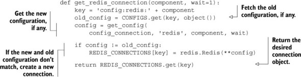
This simple function fetches the previously known as well as the current configuration. If they’re different, it updates the known configuration, creates a new connection, and then stores and returns that new connection. If the configuration hasn’t changed, it returns the previous connection.

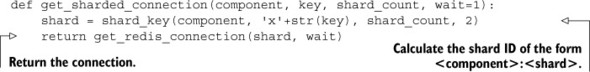
When we have the ability to fetch connections easily, we should also add support for the creation of sharded Redis connections, so even if our later decorators aren’t useful in every situation, we can still easily create and use sharded connections. To connect to a new sharded connection, we’ll use the same configuration methods, though sharded configuration will be a little different. For example, shard 7 of component logs will be stored at a key named config:redis:logs:7. This naming scheme will let us reuse the existing connection and configuration code we already have. Our function to get a sharded connection is in the following listing.

Listing 10.2. Fetch a connection based on shard information

Now that we have a simple method of fetching a connection to a Redis server that’s sharded, we can create a decorator like we saw in chapter 5 that creates a sharded connection automatically.

10.2.2. Creating a server-sharded connection decorator

Now that we have a method to easily fetch a sharded connection, let’s use it to build a decorator to automatically pass a sharded connection to underlying functions.

We’ll perform the same three-level function decoration we used in chapter 5, which will let us use the same kind of “component” passing we used there. In addition to component information, we’ll also pass the number of Redis servers we’re going to shard to. The following listing shows the details of our shard-aware connection decorator.

Listing 10.3. A shard-aware connection decorator

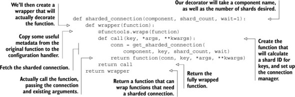
Because of the way we constructed our connection decorator, we can decorate our count_visit() function from chapter 9 almost completely unchanged. We need to be careful because we’re keeping aggregate count information, which is fetched and/or updated by our get_expected() function. Because the information stored will be used and reused on different days for different users, we need to use a nonsharded connection for it. The updated and decorated count_visit() function as well as the decorated and slightly updated get_expected() function are shown next.

Listing 10.4. A machine and key-sharded count_visit() function

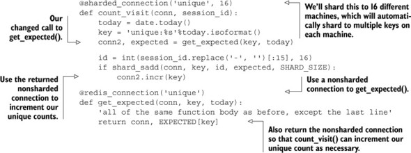
In our example, we’re sharding our data out to 16 different machines for the unique visit SETs, whose configurations are stored as JSON-encoded strings at keys named config:redis:unique:0 to config:redis:unique:15. For our daily count information, we’re storing them in a nonsharded Redis server, whose configuration information is stored at key config:redis:unique.

Multiple Redis servers on a single machine

This section discusses sharding writes to multiple machines in order to increase total memory available and total write capacity. But if you’re feeling limited by Redis’s single-threaded processing limit (maybe because you’re performing expensive searches, sorts, or other queries), and you have more cores available for processing, more network available for communication, and more available disk I/O for snapshots/AOF, you can run multiple Redis servers on a single machine. You only need to configure them to listen on different ports and ensure that they have different snapshot/AOF configurations.

Alternate methods of handling unique visit counts over time

With the use of SETBIT, BITCOUNT, and BITOP, you can actually scale unique visitor counts without sharding by using an indexed lookup of bits, similar to what we did with locations in chapter 9. A library that implements this in Python can be found at https://github.com/Doist/bitmapist.

Now that we have functions to get regular and sharded connections, as well as decorators to automatically pass regular and sharded connections, using Redis connections of multiple types is significantly easier. Unfortunately, not all operations that we need to perform on sharded datasets are as easy as a unique visitor count. In the next section, we’ll talk about scaling search in two different ways, as well as how to scale our social network example.

10.3. Scaling complex queries

As we scale out a variety of services with Redis, it’s not uncommon to run into situations where sharding our data isn’t enough, where the types of queries we need to execute require more work than just setting or fetching a value. In this section, we’ll discuss one problem that’s trivial to scale out, and two problems that take more work.

The first problem that we’ll scale out is our search engine from chapter 7, where we have machines with enough memory to hold our index, but we need to execute more queries than our server can currently handle.

10.3.1. Scaling search query volume

As we expand our search engine from chapter 7 with SORT, using the ZSET-based scored search, our ad-targeting search engine (or even the job-search system), at some point we may come to a point where a single server isn’t capable of handling the number of queries per second required. In this section, we’ll talk about how to add query slaves to further increase our capability to serve more search requests.

In section 10.1, you saw how to scale read queries against Redis by adding read slaves. If you haven’t already read section 10.1, you should do so before continuing. After you have a collection of read slaves to perform queries against, if you’re running Redis 2.6 or later, you’ll immediately notice that performing search queries will fail. This is because performing a search as discussed in chapter 7 requires performing SUNIONSTORE, SINTERSTORE, SDIFFSTORE, ZINTERSTORE, and/or ZUNIONSTORE queries, all of which write to Redis.

In order to perform writes against Redis 2.6 and later, we’ll need to update our Redis slave configuration. In the Redis configuration file, there’s an option to disable/enable writing to slaves. This option is called slave-read-only, and it defaults to yes. By changing slave-read-only to no and restarting our slaves, we should now be able to perform standard search queries against slave Redis servers. Remember that we cache the results of our queries, and these cached results are only available on the slave that the queries were run on. So if we intend to reuse cached results, we’ll probably want to perform some level of session persistence (where repeated requests from a client go to the same web server, and that web server always makes requests against the same Redis server).

In the past, I’ve used this method to scale an ad-targeting engine quickly and easily. If you decide to go this route to scale search queries, remember to pay attention to the resync issues discussed in section 10.1.

When we have enough memory in one machine and our operations are read-only (or at least don’t really change the underlying data to be used by other queries), adding slaves can help us to scale out. But sometimes data volumes can exceed memory capacity, and we still need to perform complex queries. How can we scale search when we have more data than available memory?

10.3.2. Scaling search index size

If there’s one thing we can expect of a search engine, it’s that the search index will grow over time. As search indexes grow, the memory used by those search indexes also grows. Depending on the speed of the growth, we may or may not be able to keep buying/renting larger computers to run our index on. But for many of us, getting bigger and bigger computers is just not possible.

In this section, we’ll talk about how to structure our data to support sharded search queries, and will include code to execute sharded search queries against a collection of sharded Redis masters (or slaves of sharded masters, if you followed the instructions in section 10.3.1).

In order to shard our search queries, we must first shard our indexes so that for each document that we index, all of the data about that document is on the same shard. It turns out that our index_document() function from chapter 7 takes a connection object, which we can shard by hand with the docid that’s passed. Or, because index_document() takes a connection followed by the docid, we can use our automatic sharding decorator from listing 10.3 to handle sharding for us.

When we have our documents indexed across shards, we only need to perform queries against the shards to get the results. The details of what we need to do will depend on our type of index—whether it’s SORT-based or ZSET-based. Let’s first update our SORT-based index for sharded searches.

Sharding SORT-based search

As is the case with all sharded searches, we need a way to combine the results of the sharded searches. In our implementation of search_and_sort() from chapter 7, we received a total count of results and the document IDs that were the result of the required query. This is a great building block to start from, but overall we’ll need to write functions to perform the following steps:

1.  Perform the search and fetch the values to sort on for a query against a single shard.

2.  Execute the search on all shards.

3.  Merge the results of the queries, and choose the subset desired.

First, let’s look at what it takes to perform the search and fetch the values from a single shard.

Because we already have search_and_sort() from chapter 7, we can start by using that to fetch the result of a search. After we have the results, we can then fetch the data associated with each search result. But we have to be careful about pagination, because we don’t know which shard each result from a previous search came from. So, in order to always return the correct search results for items 91–100, we need to fetch the first 100 search results from every shard. Our code for fetching all of the necessary results and data can be seen in the next listing.

Listing 10.5. SORT-based search that fetches the values that were sorted

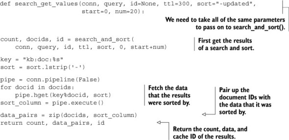
This function fetches all of the information necessary from a single shard in preparation for the final merge. Our next step is to execute the query on all of the shards.

To execute a query on all of our shards, we have two options. We can either run each query on each shard one by one, or we can execute our queries across all of our shards simultaneously. To keep it simple, we’ll execute our queries one by one on each shard, collecting the results together in the next listing.

Listing 10.6. A function to perform queries against all shards

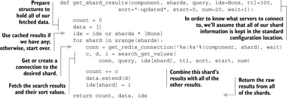
This function works as explained: we execute queries against each shard one at a time until we have results from all shards. Remember that in order to perform queries against all shards, we must pass the proper shard count to the get_shard_results() function.

Now that we have all of the results from all of the queries, we only need to re-sort our results so that we can get an ordering on all of the results that we fetched. This isn’t terribly complicated, but we have to be careful about numeric and non-numeric sorts, handling missing values, and handling non-numeric values during numeric sorts. Our function for merging results and returning only the requested results is shown in the next listing.

Listing 10.7. A function to merge sharded search results

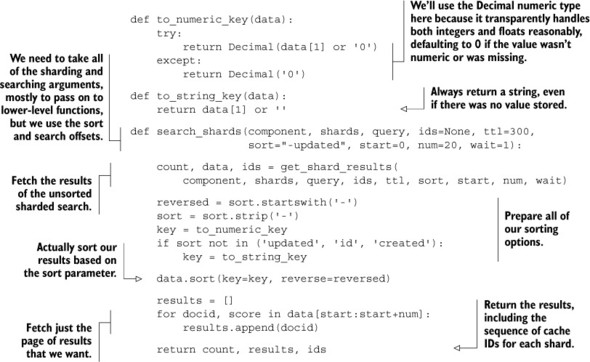
In order to handle sorting properly, we needed to write two function to convert data returned by Redis into values that could be consistently sorted against each other. You’ll notice that we chose to use Python Decimal values for sorting numerically. This is because we get the same sorted results with less code, and transparent support for handling infinity correctly. From there, all of our code does exactly what’s expected: we fetch the results, prepare to sort the results, sort the results, and then return only those document IDs from the search that are in the requested range.

Now that we have a version of our SORT-based search that works across sharded Redis servers, it only remains to shard searching on ZSET-based sharded indexes.

Sharding ZSET-based search

Like a SORT-based search, handling searching for ZSET-based search requires running our queries against all shards, fetching the scores to sort by, and merging the results properly. We’ll go through the same steps that we did for SORT-based search in this section: search on one shard, search on all shards, and then merge the results.

To search on one shard, we’ll wrap the chapter 7 search_and_zsort() function on ZSETs, fetching the results and scores from the cached ZSET in the next listing.

Listing 10.8. ZSET-based search that returns scores for each result

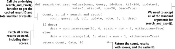
Compared to the SORT-based search that does similar work, this function tries to keep things simple by ignoring the returned results without scores, and just fetches the results with scores directly from the cached ZSET. Because we have our scores already as floating-point numbers for easy sorting, we’ll combine the function to search on all shards with the function that merges and sorts the results.

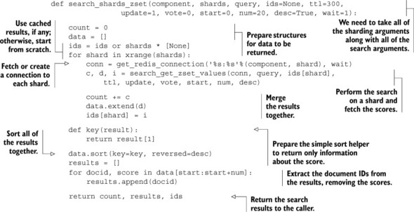
As before, we’ll perform searches for each shard one at a time, combining the results. When we have the results, we’ll sort them based on the scores that were returned. After the sort, we’ll return the results to the caller. The function that implements this is shown next.

Listing 10.9. Sharded search query over ZSETs that returns paginated results

With this code, you should have a good idea of the kinds of things necessary for handling sharded search queries. Generally, when confronted with a situation like this, I find myself questioning whether it’s worth attempting to scale these queries in this way. Given that we now have at least working sharded search code, the question is easier to answer. Note that as our number of shards increase, we’ll need to fetch more and more data in order to satisfy our queries. At some point, we may even need to delegate fetching and merging to other processes, or even merging in a tree-like structure. At that point, we may want to consider other solutions that were purpose-built for search (like Lucene, Solr, Elastic Search, or even Amazon’s Cloud Search).

Now that you know how to scale a second type of search, we really have only covered one other problem in other sections that might reach the point of needing to be scaled. Let’s take a look at what it would take to scale our social network from chapter 8.

10.3.3. Scaling a social network

As we built our social network in chapter 8, I pointed out that it wasn’t designed to scale to the size of a social network like Twitter, but that it was primarily meant to help you understand what structures and methods it takes to build a social network. In this section, I’ll describe a few methods that can let us scale a social networking site with sharding, almost without bounds (mostly limited by our budget, which is always the case with large projects).

One of the first steps necessary to helping a social network scale is figuring out what data is read often, what data is written often, and whether it’s possible to separate often-used data from rarely used data. To start, say that we’ve already pulled out our posted message data into a separate Redis server, which has read slaves to handle the moderately high volume of reads that occurs on that data. That really leaves two major types of data left to scale: timelines and follower/following lists.

Scaling posted message database size

If you actually built this system out, and you had any sort of success, at some point you’d need to further scale the posted message database beyond just read slaves. Because each message is completely contained within a single HASH, these can be easily sharded onto a cluster of Redis servers based on the key where the HASH is stored. Because this data is easily sharded, and because we’ve already worked through how to fetch data from multiple shards as part of our search scaling in section 10.3.2, you shouldn’t have any difficulty here. Alternatively, you can also use Redis as a cache, storing recently posted messages in Redis, and older (rarely read) messages in a primarily on-disk storage server (like PostgreSQL, MySQL, Riak, MongoDB, and so on). If you’re finding yourself challenged, please feel free to post on the message board or on the Redis mailing list.

As you may remember, we had three primary types of timelines: home timelines, profile timelines, and list timelines. Timelines themselves are all similar, though both list timelines and home timelines are limited to 1,000 items. Similarly, followers, following, list followers, and list following are also essentially the same, so we’ll also handle them the same. First, let’s look at how we can scale timelines with sharding.

Sharding timelines

When we say that we’re sharding timelines, it’s a bit of a bait-and-switch. Because home and list timelines are short (1,000 entries max, which we may want to use to inform how large to set zset-max-ziplist-size),^[1] there’s really no need to shard the contents of the ZSETs; we merely need to place those timelines on different shards based on their key names.

¹ Because of the way we add items to home and list timelines, they can actually grow to roughly 2,000 entries for a short time. And because Redis doesn’t turn structures back into ziplist-encoded versions of themselves when they’ve gotten too large, setting zset-max-ziplist-size to be a little over 2,000 entries can keep these two timelines encoded efficiently.

On the other hand, the size that profile timelines can grow to is currently unlimited. Though the vast majority of users will probably only be posting a few times a day at most, there can be situations where someone is posting significantly more often. As an example of this, the top 1,000 posters on Twitter have all posted more than 150,000 status messages, with the top 15 all posting more than a million messages.

On a practical level, it wouldn’t be unreasonable to cap the number of messages that are kept in the timeline for an individual user to 20,000 or so (the oldest being hidden or deleted), which would handle 99.999% of Twitter users generally. We’ll assume that this is our plan for scaling profile timelines. If not, we can use the technique we cover for scaling follower/following lists later in this section for scaling profile timelines instead.

In order to shard our timelines based on key name, we could write a set of functions that handle sharded versions of ZADD, ZREM, and ZRANGE, along with others, all of which would be short three-line functions that would quickly get boring. Instead, let’s write a class that uses Python dictionary lookups to automatically create connections to shards.

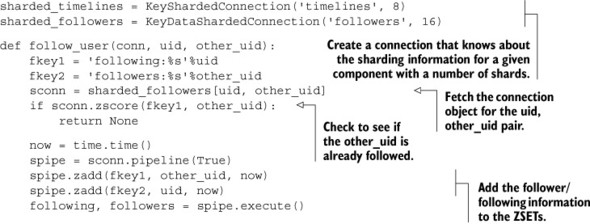
First, let’s start with what we want our API to look like by updating our follow_user() function from chapter 8. We’ll create a generic sharded connection object that will let us create a connection to a given shard, based on a key that we want to access in that shard. After we have that connection, we can call all of the standard Redis methods to do whatever we want on that shard. We can see what we want our API to look like, and how we need to update our function, in the next listing.

Listing 10.10. An example of how we want our API for accessing shards to work

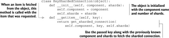
Now that we have an idea of what we want our API to look like, let’s build it. We first need an object that takes the component and number of shards. When a key is referenced via dictionary lookup on the object, we need to return a connection to the shard that the provided key should be stored on. The class that implements this follows.

Listing 10.11. A class that implements sharded connection resolution based on key

For simple key-based sharding, this is all that’s necessary to support almost every call that we’d perform in Redis. All that remains is to update the remainder of unfollow_user(), refill_timeline(), and the rest of the functions that access home timelines and list timelines. If you intend to scale this social network, go ahead and update those functions yourself. For those of us who aren’t scaling the social network, we’ll continue on.

Up next is scaling follower and following lists.

Scaling follower and following lists with sharding

Though our scaling of timelines is pretty straightforward, scaling followers, following, and the equivalent “list” ZSETs is more difficult. The vast majority of these ZSETs will be short (99.99% of users on Twitter have fewer than 1,000 followers), but there may be a few users who are following a large number of users, or who have a large number of followers. As a practical matter, it wouldn’t be unreasonable to limit the number of users that a given user or list can follow to be somewhat small (perhaps up to 1,000, to match the limits on home and list timelines), forcing them to create lists if they really want to follow more people. But we still run into issues when the number of followers of a given user grows substantially.

To handle the situation where follower/following lists can grow to be very large, we’ll shard these ZSETs across multiple shards. To be more specific, a user’s followers will be broken up into as many pieces as we have shards. For reasons we’ll get into in a moment, we only need to implement specific sharded versions of ZADD, ZREM, and ZRANGEBYSCORE.

I know what you’re thinking: since we just built a method to handle sharding automatically, we could use that. We will (to some extent), but because we’re sharding data and not just keys, we can’t just use our earlier class directly. Also, in order to reduce the number of connections we need to create and call, it makes a lot of sense to have data for both sides of the follower/following link on the same shard, so we can’t just shard by data like we did in chapter 9 and in section 10.2.

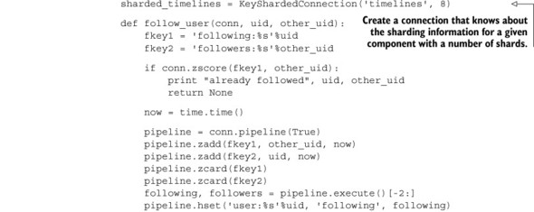
In order to shard our follower/following data such that both sides of the follower/following relationship are on the same shard, we’ll use both IDs as part of the key to look up a shard. Like we did for sharding timelines, let’s update follow_user() to show the API that we’d like to use, and then we’ll create the class that’s necessary to implement the functionality. The updated follow_user() with our desired API is next.

Listing 10.12. Access follower/following ZSET shards

Aside from a bit of rearrangement and code updating, the only difference between this change and the change we made earlier for sharding timelines is that instead of passing a specific key to look up the shard, we pass a pair of IDs. From these two IDs, we’ll calculate the proper shard that data involving both IDs should be stored on. The class that implements this API appears next.

Listing 10.13. Sharded connection resolution based on ID pairs

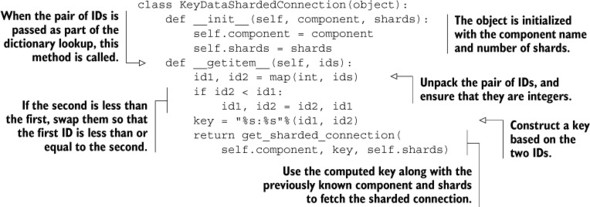
The only thing different for this sharded connection generator, compared to listing 10.11, is that this sharded connection generator takes a pair of IDs instead of a key. From those two IDs, we generate a key where the lower of the two IDs is first, and the higher is second. By constructing the key in this way, we ensure that whenever we reference the same two IDs, regardless of initial order, we always end up on the same shard.

With this sharded connection generator, we can update almost all of the remaining follower/following ZSET operations. The one remaining operation that’s left is to properly handle ZRANGEBYSCORE, which we use in a few places to fetch a “page” of followers. Usually this is done to syndicate messages out to home and list timelines when an update is posted. When syndicating to timelines, we could scan through all of one shard’s ZSET, and then move to the next. But with a little extra work, we could instead pass through all ZSETs simultaneously, which would give us a useful sharded ZRANGEBYSCORE operation that can be used in other situations.

As we saw in section 10.3.2, in order to fetch items 100–109 from sharded ZSETs, we needed to fetch items 0–109 from all ZSETs and merge them together. This is because we only knew the index that we wanted to start at. Because we have the opportunity to scan based on score instead, when we want to fetch the next 10 items with scores greater than X, we only need to fetch the next 10 items with scores greater than X from all shards, followed by a merge. A function that implements ZRANGEBYSCORE across multiple shards is shown in the following listing.

Listing 10.14. A function that implements a sharded ZRANGEBYSCORE

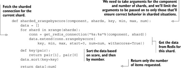
This function works a lot like the query/merge that we did in section 10.3.2, only we can start in the middle of the ZSET because we have scores (and not indexes).

Using this method for sharding profile timelines

You’ll notice that we use timestamps for follower/following lists, which avoided some of the drawbacks to paginate over sharded ZSETs that we covered in section 10.3.2. If you’d planned on using this method for sharding profile timelines, you’ll need to go back and update your code to use timestamps instead of offsets, and you’ll need to implement a ZREVRANGEBYSCORE version of listing 10.14, which should be straightforward.

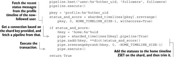
With this new sharded ZRANGEBYSCORE function, let’s update our function that syndicates posts to home and list timelines in the next listing. While we’re at it, we may as well add support for sharded home timelines.

Listing 10.15. Updated syndicate status function

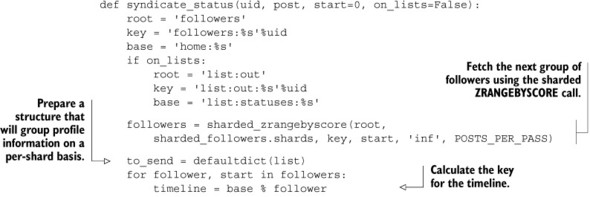
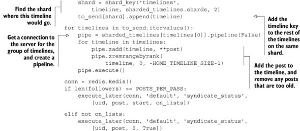
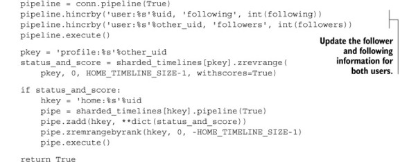
As you can see from the code, we use the sharded ZRANGEBYSCORE function to fetch those users who are interested in this user’s posts. Also, in order to keep the syndication process fast, we group requests that are to be sent to each home or list timeline shard server together. Later, after we’ve grouped all of the writes together, we add the post to all of the timelines on a given shard server with a pipeline. Though this may be slower than the nonsharded version, this does allow us to scale our social network much larger than before.

All that remains is to finish updating the rest of the functions to support all of the sharding that we’ve done in the rest of section 10.3.3. Again, if you’re going to scale this social network, feel free to do so. But if you have some nonsharded code that you want to shard, you can compare the earlier version of syndicate_status() from section 8.4 with our new version to get an idea of how to update your code.

10.4. Summary

In this chapter, we revisited a variety of problems to look at what it’d take to scale them to higher read volume, higher write volume, and more memory. We’ve used read-only slaves, writable query slaves, and sharding combined with shard-aware classes and functions. Though these methods may not cover all potential use cases for scaling your particular problem, each of these examples was chosen to offer a set of techniques that can be used generally in other situations.

If there’s one concept that you should take away from this chapter, it’s that scaling any system can be a challenge. But with Redis, you can use a variety of methods to scale your platform (hopefully as far as you need it to scale).

Coming up in the next and final chapter, we’ll cover Redis scripting with Lua. We’ll revisit a few past problems to show how our solutions can be simplified and performance improved with features available in Redis 2.6 and later.