4

Graphics and Game Engine Components

No matter which graphics or games development engine you examine, they are built using a very similar architecture, the reason being that they all have to work with the same graphics devices, central processing units (CPUs), and graphics processing units (GPUs) to produce stunning visuals with exceptional frame rates. If you consider the nature of graphical elements that are drawn on a screen, they are also constructed from numerous layers depending on their functionality, dimensions in pixels, coloring, animation, lighting, physics, and user interaction.

In this chapter, we will begin exploring some typical application architectures as we begin to build our own. To enable the drawing of three-dimensional (3D) objects in Python we will use the PyOpenGL package that implements OpenGL (a 3D graphics library). You will learn how each of the graphics components works together to create a scalable and flexible graphics engine.

Herein, we will cover the following topics:

• Exploring the OpenGL Graphics Pipeline
• Drawing Models with Meshes
• Viewing the Scene with Cameras
• Projecting Pixels onto the Screen
• Understanding 3D Coordinate Systems in OpenGL

Technical requirements

In this chapter, we will be using Python, PyCharm, and Pygame, as used in previous chapters.

Before you begin coding, create a new folder in the PyCharm project for the contents of this chapter, called Chapter_4.

You will also need PyOpenGL, the installation of which will be covered during the first exercise.

The solution files containing the code can be found on GitHub at https://github.com/PacktPublishing/Mathematics-for-Game-Programming-and-Computer-Graphics/tree/main/Chapter04.

Exploring the OpenGL Graphics Pipeline

In software, an engine is an application that takes all the hard work out of creating an application by providing an application programming interface (API) specific to the task. Unity3D, for example, is a game engine. It’s a tool for creating games and empowers the programmer by removing the need to write low-level code.

An engine consists of several modules dedicated to tasks, as shown in Figure 4.1:

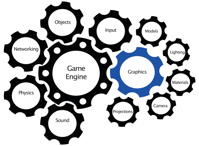
Figure 4.1: Typical components of a game engine

A mainstream graphics application needs to possess all the fundamental abilities to display and move graphics elements (such as the ones we examined in Chapter 2, Let’s Start Drawing) in either 2D or 3D, with most 3D engines able to display 2D simply by removing the z axis. These elements work together to take a 2D or 3D model through the graphics pipeline where it is transformed from a set of vertices into an image that appears on the screen. The graphics pipeline includes several highly mathematical steps to achieve the final product. These steps are illustrated in the following diagram:

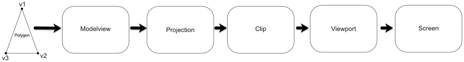
Figure 4.2: Graphics pipeline

Let’s look at each of these steps here:

• First, the vertices of the model to be drawn are transformed by the modelview into camera space (also called eye space). This changes the model’s vertices, edges, and other characteristics relative to the camera’s location and other properties. At this point, the model color information is attached to each vertex.
• The vertices and colors are then passed to the projection, which transforms the values into a view volume. At this point in the pipeline, the model has been reduced to pixels.
• Clipping then discards any drawing information that is outside the viewing volume of the camera as it is no longer required. It can’t be seen, so why draw it?
• Then, the viewport takes the pixel information and transforms it yet again into device-specific coordinates of the output device, and the pixel information is seen on the screen.

We will revisit sections of the graphics pipeline as we move forward with examples that will assist your understanding.

First, however, we are going to set up PyCharm with OpenGL to allow us to create more advanced 3D graphics programs as we move forward. OpenGL is a cross-platform, freely available API for interacting with the GPU to achieve hardware-accelerated drawing and has been an industry standard since the early 1990s.

Let’s do it…

In this exercise, we will walk through the process to get Python’s OpenGL package installed and tested. Before you begin, as already mentioned, create a new folder in PyCharm to store the code from this chapter. Then, complete these steps:

1. In PyCharm, go to the Python Packages window and install PyOpenGL (in the same way we installed Pygame). The correct package to install is shown in Figure 4.3:

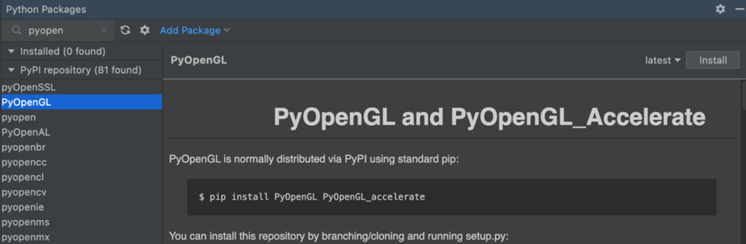
Figure 4.3: Installing PyOpenGL in PyCharm

2. Create a new Python file called OpenGLStarter.py and add the following code to it:

   import pygame

   from pygame.locals import *

   from OpenGL.GL import *

   pygame.init()

   screen_width = 500

   screen_height = 500

   screen = pygame.display.set_mode((screen_width,

                                     screen_height),

                                     DOUBLEBUF|OPENGL)

   pygame.display.set_caption('OpenGL in Python')

   done = False

   white = pygame.Color(255, 255, 255)

   while not done:

     for event in pygame.event.get():

       if event.type == pygame.QUIT:

         done = True

     glClear(GL_COLOR_BUFFER_BIT | GL_DEPTH_BUFFER_BIT)

     pygame.display.flip()

   pygame.quit()

When run, this code will open up a window as before. Note that much of what we’ve already been working with is still the same; however, the noticeable differences are set out here:

• DOUBLEBUF|OPENGL option in set_mode(): We have moved from drawing a single image buffer to a double buffer and asked Pygame to use OpenGL to perform the rendering. A double buffer is required when drawing animated objects, as we will be doing later in this book. It means that one image is on the screen while another is being drawn behind the scenes.
• glClear() inside the while loop: glClear() clears the screen using the GL_COLOR_BUFFER_BIT | GL_DEPTH_BUFFER_BIT bitmask, which removes color and depth information.
• pygame.display.flip(): Here, flip() replaces the update() method we previously used and switches the buffer images so that the background buffer is sent to the screen.

For in-depth information on any OpenGL methods introduced, the interested reader is encouraged to visit the following web page:

https://www.khronos.org/registry/OpenGL-Refpages/gl4/

This script will now become the new starter file for our projects. Whenever a new Python project is started, be sure to copy this code into the new file unless otherwise directed.

With the basic program that we will be working with developed, it’s time to look at some graphics/game engine modules, in turn adding their basic functionality to our Python application as we proceed.

Drawing Models with Meshes

A model is an object drawn by the graphics engine. It contains a list of vertices that define its structure in terms of polygons. The collection of these connected polygons is known as a mesh. Each polygon inhabits a plane—this means that it is flat. A basic model with elementary shading appears faceted, such as that shown in Figure 4.4. This flat nature is hidden using differing materials, as we will discuss shortly:

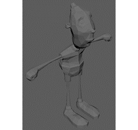
Figure 4.4: A basic polygon mesh showing the flatness of each polygon

A polygon mesh is stored internally as a list of vertices and triangles. Triangles are chosen to represent each polygon over that of a square, as triangles require less storage and are faster to manipulate as they have one less vertex.

A typical data structure to hold a mesh is illustrated in the following diagram:

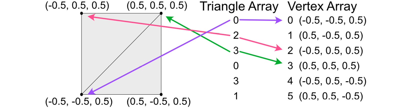
Figure 4.5: A vertex and triangle array used to define the triangles of a square

The example given stores a square split into two triangles. The vertex array holds all the vertices of the shape. Another array stores a series of integers that are grouped in threes and store the three vertices of a triangle. You can see how the first triangle (group of three values) in the triangle array references the indices of the vertex array, thus allowing a polygon to be defined.

The code to store the data for a mesh as shown in Figure 4.5 is straightforward, as you are about to discover.

Let’s do it…

We will now define a mesh class and integrate it into our project, as follows:

1. Create a new Python file called HelloMesh.py and add in the basic OpenGL starter code we created in the previous exercise.
2. Create another Python file called Mesh3D.py and add the following code to it:

   from OpenGL.GL import *

   class Mesh3D:

     def __init__(self):

       self.vertices = [(0.5, -0.5, 0.5),

               (-0.5, -0.5, 0.5),

               (0.5, 0.5, 0.5),

               (-0.5, 0.5, 0.5),

               (0.5, 0.5, -0.5),

               (-0.5, 0.5, -0.5)

               ]

       self.triangles = [0, 2, 3, 0, 3, 1]

     def draw(self):

       for t in range(0, len(self.triangles), 3):

             glBegin(GL_LINE_LOOP)

             glVertex3fv(

                 self.vertices[self.triangles[t]])

             glVertex3fv(self.vertices[self.triangles[t +

                         1]])

             glVertex3fv(self.vertices[self.triangles[t +

                         2]])

             glEnd()

In the class constructor, the vertices and triangles are hardcoded, and we will come back and change these later to something more flexible. The draw method allows this class to draw out the given triangles as a series of triangles. It loops through three vertices at a time and uses GL_LINE_LOOP to connect each.

OpenGL draws in blocks, starting with glBegin() and ending with glEnd(). The glBegin() parameter tells OpenGL how to draw. In this case, it is a line that goes from vertex to vertex and then reconnects itself with the first vertex.

3. To see the drawing in action, modify HelloMesh.py thus:

   import pygame

   from Mesh3D import *

   from pygame.locals import *

   ..

   mesh = Mesh3D()

   while not done:

     for ..

     glClear(GL_COLOR_BUFFER_BIT | GL_DEPTH_BUFFER_BIT)

     mesh.draw()

     pygame.display.flip()

   ..

With these changes, you are adding a mesh into your project and then ensuring it is drawn in the main loop.

4. Run HelloMesh.py to see the result, as illustrated in Figure 4.6:

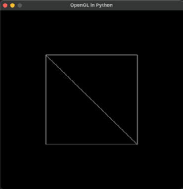
Figure 4.6: Drawing a square mesh with two triangles

Your turn…

Exercise A: Consider the mesh drawn in the previous section as the top of a cube. This cube extends from (-0.5, -0.5, -0.5) to (0.5, 0.5, 0.5). Define values for the vertices and triangles arrays, and create a class called Cube that inherits from Mesh3D and that will draw this new cubic mesh. (Hint: you only need to define the vertices and triangles; the draw() method will work as is.)

The code should begin like this:

from Mesh3D import *
class Cube(Mesh3D):
  def __init__(self):
    self.vertices = (insert vertices)..
    self.triangles = (insert triangles)..

Thus far in our project, we’ve not had a lot of influence over the location of the mesh within the 3D space or how we are looking at it. To allow for a better view of the cube or manipulate where it is appearing on the screen, we now need to consider the concept of cameras before adding them to the code.

Viewing the Scene with Cameras

The camera is responsible for taking the coordinates of objects (specifically, all their vertices and other properties) and transforming them in the modelview of Figure 4.2. If you consider the vertices of the square mesh we looked at in the previous section, its coordinates are not going to retain those values as it will be moved around in the graphics/game world. The modelview takes the world location of the mesh and the location of the camera, as well as some additional properties, and determines the new coordinates of the mesh so that it can be rendered correctly. Note that I am being purposefully abstract in describing this process right now as there’s a lot of mathematics involved, and I don’t want to complicate the discussion at this point!

The camera is a virtual object through which the world is visualized. It is the eye of the viewer and can be moved around the environment to provide different points of view. As illustrated in the following screenshot, the camera consists of a near plane that represents the screen where pixels are drawn, and a far plane that determines how far back into the world the camera can see:

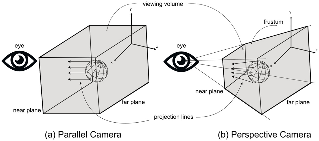
Figure 4.7: A camera with a perspective view

Any objects in front of the near plane or behind the far plane are culled. The area contained between the near and far planes is called the viewing volume.

The shape of the viewing volume differs between camera types and influences how a scene is rendered on the screen, as illustrated in Figure 4.8. Essentially, there are two camera types: parallel (also called orthogonal) and perspective. The shape of the viewing volume for a parallel camera is a rectangular prism, whereas, for perspective, it is called a frustum, which is a four-sided pyramid with the top cut off. This frustum can be seen in Figure 4.8a. In parallel, all objects inside the viewing volume are projected by straight lines at the near plane to be drawn. Unlike our own natural viewing of the real world where objects that are further away look smaller, in parallel, all objects retain their original scaling, no matter how far away they are from the eye. The other type of camera, shown in Figure 4.8b, gives a perspective view. This is closer to our own viewing outlook. This is illustrated in Figure 4.8c, where the scene containing several spheres that are all the same size but at different distances from the camera (a) appears to be all the same size in the parallel view of (b) but appears to look more natural in perspective (c):

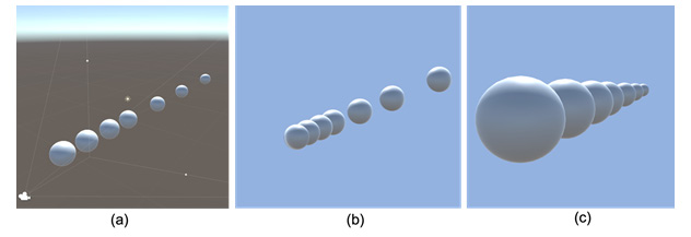
Figure 4.8: A 3D scene (a) viewed in parallel (b) and perspective (c)

When we look out into the world, for a person with normal eyesight, because our eyes are situated horizontally, we see the world as being wider than it is tall. If you were to hold your arms horizontally out from your sides while looking straight ahead and then slowly bring your arms around to your front, the moment that you can see your hands measures your field of view (FOV). For the average human, this is around 60 degrees. The virtual camera also has a field of view (FOV) whose value determines the horizontal resolution of the virtual world. It is this value that sets the angle of the projection lines in the perspective view and affects the scale of the world, as seen in Figure 4.9. A narrow field of view showing what the camera sees on the left and the camera frustum on the right is shown in (a) and a wide field of view with the same camera point of view and frustum view is presented in (b):

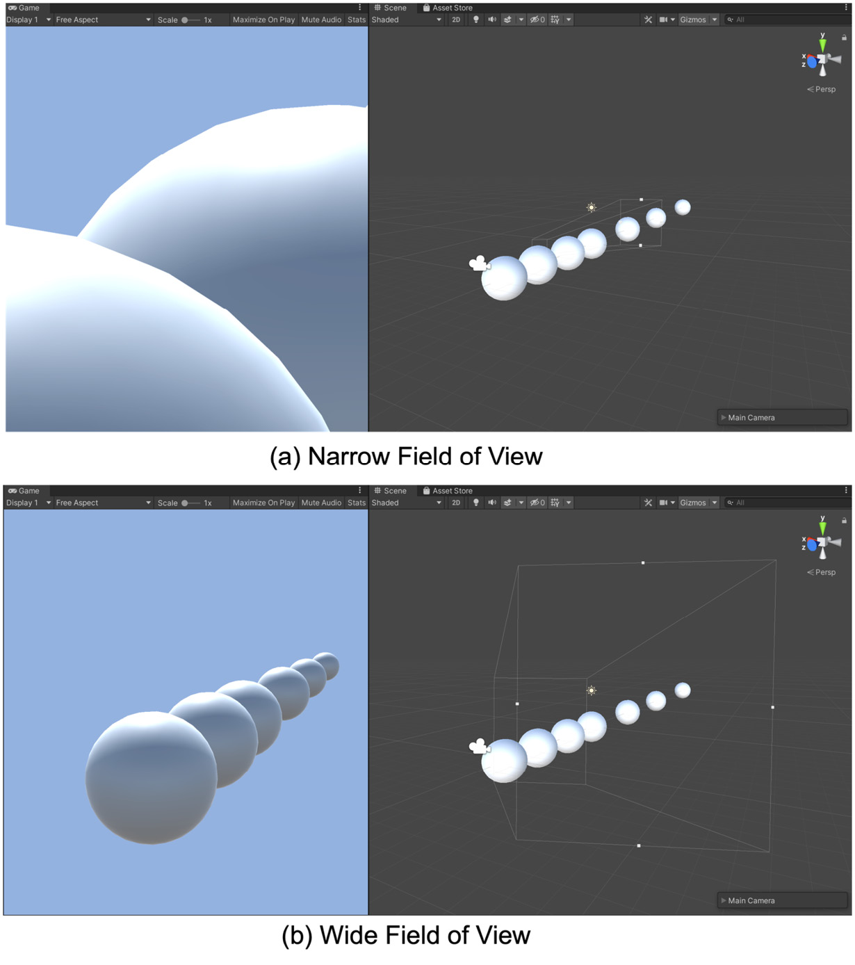
Figure 4.9: Different FOVs demonstrated by a camera in the Unity game engine

The FOV for a virtual camera has traditionally been set for the horizontal because of the way humans see the world, though mathematically, there’s no reason why the vertical direction couldn’t be set; we will stick with the horizontal FOV herein, however. With the horizontal FOV set, the vertical FOV is calculated from the screen resolution using the following equation:

vertical_fov = horizontal_fov * screen.height / screen.width)

This ensures correct scaling of the environment to ensure the camera’s near plane dimensions are a consistent scale of the screen dimensions. Imagine if the camera’s near plane were a perfect square and you tried to map this onto a typical 1,920 x 1,080 screen. It would have to stretch the camera’s view in the x direction while the y direction remained unaffected.

The mathematical processes that take the vertices of a model and how they are viewed by the camera finally make it into screen coordinates via projections.

Projecting Pixels onto the Screen

As previously discussed, the function of a projection is to map coordinates in the eye space into a rectangular prism with the corner coordinates of (-1, -1, -1) and (1, 1, 1), as shown in Figure 4.10. This volume is called normalized device coordinates (NDCs). This cube is used to define coordinates in a screen-independent display coordinate system and defines the view volume as normalized points. This information can then be used to produce pixels on the screen with the z coordinates being used during the drawing to determine which pixels should appear in front of others. First, though, you need to define the confines of the camera’s view volume so that a mapping can be produced:

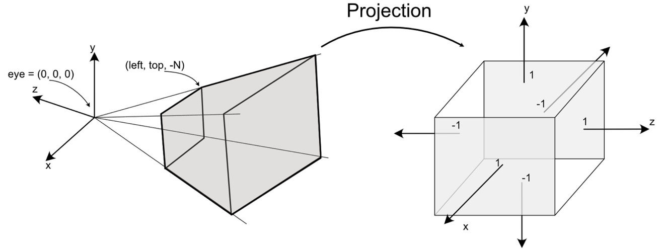
Figure 4.10: The process of projection

Since the object is projected onto the near plane of the camera, we can use the corner coordinates of that plane to determine the mapping. The coordinates of the left top corner are indicated by (left, top, -N) where N is the distance of the near plane from the camera’s eye. Note that N in this case is negative as the positive direction of the z axis is toward the viewer. Why? To understand this, we must take a brief tangent in our discussion to examine coordinate systems.

Understanding 3D Coordinate Systems in OpenGL

There are two alignments in which 3D coordinates can be defined: the left-handed system and the right-handed system. Each is used to define the direction in which rotations around the axes occur and can be visualized using the thumb and first two fingers on the respective hands (see Figure 4.11). For both systems, the thumb is used to represent the z axis; the direction in which the fingers wrap into a fist is the direction of a positive rotation:

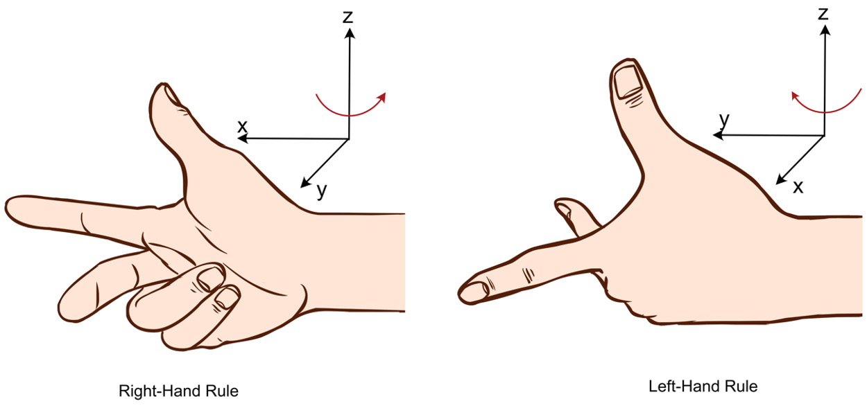
Figure 4.11: The right-hand and left-hand rules of 3D axis orientation

For a detailed elucidation, you are encouraged to read the following web page:

https://en.wikipedia.org/wiki/Right-hand_rule

In OpenGL, eye coordinates are defined using the right-handed system, meaning that the positive z axis protrudes out of the screen (toward the eye) whereas traditionally in DirectX, the z axis is positive in the opposite direction. Other 3D software packages seem to have randomly chosen which coordinate system to use. For example, Blender adheres to the right-hand rule, and Unity3D is left-handed. The reason for the use of differing rules is simply that no standard exists to define what should be used.

Perspective Projection

A perspective projection is how our human eyes view the world, whereby objects get smaller the further they are away from us. We will consider the mathematics of a perspective projection for projecting a point from eye space into NDC using the right-handed system (simply because I’m more familiar with OpenGL than DirectX!). This means eye coordinates are defined with the positive z axis coming out of the screen and placing the camera’s near plane z coordinate at -N.

To work out the value of left, we make a right-angled triangle between the eye and the middle of the near plane, as shown in Figure 4.12. Where the right angle occurs has an x value of 0, with left being in the negative x direction and right in the positive x direction:

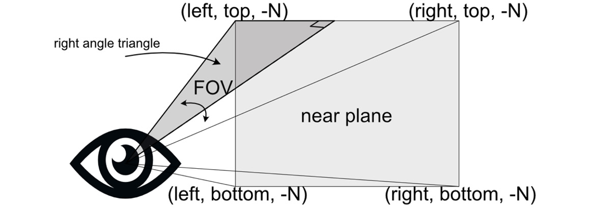
Figure 4.12: The coordinates of the camera’s near plane and constructing a right-angle triangle

As the value of N is known, using the rules of trigonometry (see Chapter 8, Reviewing Our Knowledge of Triangles), we can calculate the following:

left = -tan(horizontal_fov / 2) * -N
right = tan(horizontal_fov / 2) * -N

left can further be defined as follows:

left = -right

Note that we divide the FOV by 2 as the right-angle triangle only uses half the angle.

Next, to calculate the values of top and bottom, we can do the same thing except with vertical_fov, like so:

top = tan(vertical_fov/2) * -N
bottom = -tan(vertical_fov/2) * -N

At this point, we have the coordinates for all the corners of the near plane. From here, we can calculate the following:

nearplane_width = right - left
nearplane_height = top – bottom

Let’s look at an example of working with these values.

To calculate the left and top values of a camera, as shown in Figure 4.12, with a horizontal_fov value of 60, a near plane of 0.03, and a screen resolution of 1920 x 1080, first we must work out the vertical_fov value. Recall this is obtained like so:

vertical_fov = horizontal_fov * screen.height / screen.width)

For this camera, that makes vertical_fov equal to 33.75. We can then calculate left as -tan(30) x 0.03, which is -0.017, and top as tan(33.75/2), which is 0.3. But don’t take my word for it. Calculate it yourself.

Hint

When working with mathematics that returns values that can be plotted or illustrated, don’t take the values you calculate at face value. You can provide some validation to the numbers you are getting by considering whether they make sense. Draw a diagram and have a look. For example, if a widescreen has a horizontal_fov of 60 then, its vertical_fov is first going to be smaller, and considering the screen resolution where the height is kind of close to half the width, then a vertical_fov of around half the horizontal_fov makes sense.

The calculations presented in this section are essential for when you want to develop your own perspective projections. By working logically through the trigonometry involved in defining the near plane of a camera based on the FOV, we have explored how to derive these equations that will later be used to program a camera.

Your turn…

Exercise B: What are the right and bottom values for a camera’s near plane corners if the horizontal_fov is 80, the near plane is 2, and the screen resolution is 1,366 x 768?

Projecting into the NDC

With the near-plane extents defined, we then project the point from eye space into the NDC. This process is illustrated in the next screenshot and progresses thus:

• First, a point (labeled 1 in Figure 4.13) in eye space is projected forward onto the near plane of the camera (labeled 2).
• Then, the point is mapped onto the near plane of the NDC (labeled 3). This process uses the ratio of the point’s location to the width and height of the near plane to place it in the same relative location on the front plane of the NDC.
• The point is then given a depth value to push it back into the NDC (labeled 4):

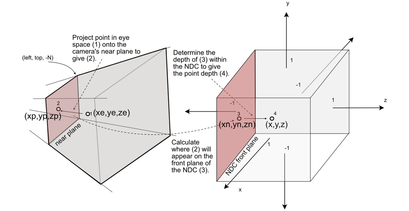
Figure 4.13: The projection process – the steps involved in taking a point from the eye space into the NDC

The point actually stays on the front face of the NDC as this is eventually mapped to the screen coordinates of the device through which the point is being viewed. The depth information is stored purely to determine which points are in front of others and thus which points to cull from drawing if they are behind others and can’t be seen.

Points are first projected onto the near plane of the camera where (xe, ye, ze) becomes (xp, yp, zp), as illustrated in Figure 4.13. We can work out this projection for the x coordinates and y coordinates separately. This is a straightforward process, using the ratios of similar triangles illustrated in Figure 4.14.

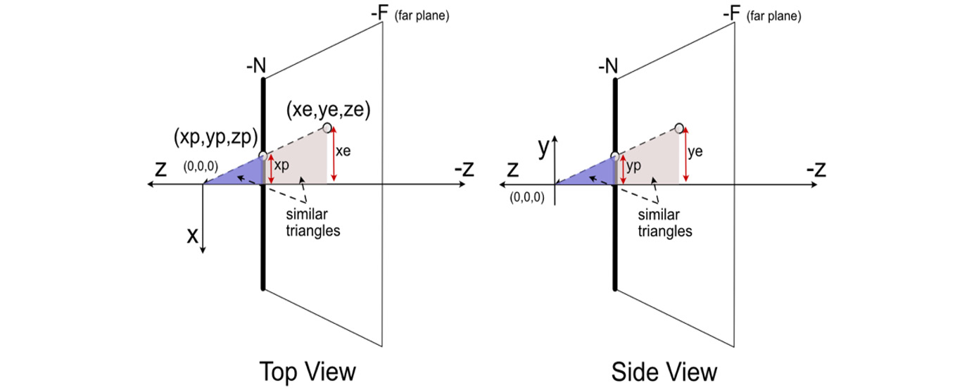
Figure 4.14: Top and side views demonstrating the projection of the x and y values of a point

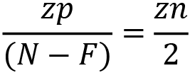
xp and yp can be calculated thus:

When a point is projected onto the near plane, its z value becomes -N. Therefore, the formula looks like this:

The illustration in Figure 4.15 showing the x and y dimensions of the near plane and NDC front plane. The location of the same point is on the left on the near plane and on the right on the NDC front plane. Each illustration shows the height and width of each plane:

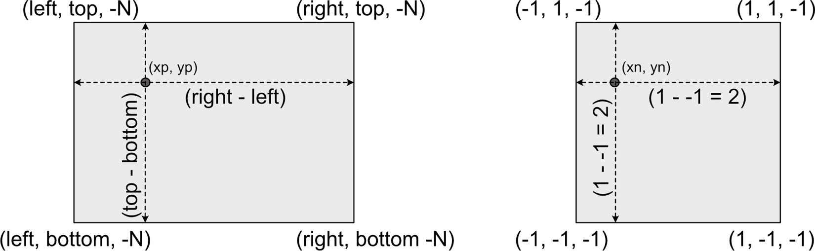
Figure 4.15: A front view of the perspective near plane and NDC front plane

Next, the point (xp, yp, zp) is projected onto the front plane of the NDC to produce (xn, yn, zn), as shown in Figure 4.15. Solving this problem involves remapping each of the x, y, and z values as a ratio to the respective size of the camera space in each dimension and then determining what this ratio equates to in the NDC.

When the remapping from one plane to another occurs, the ratio of the point to the size of its plane should remain constant. This means that the following formula applies:

Put simply, if the value of xp were 20% of the way width-wise across the camera’s near plane, then the value of xn would be 20% across the width of the NDC.

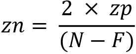
Rearranging to solve for xn and yn, we get the following:

The value for zn can be calculated in the same manner, but instead of using the height and width of a space, the distance in the depth of the space is used thus:

And through rearranging, we get the following:

OpenGL takes care of all this mathematics behind the scenes when drawing vertices and figures to the screen. In the next exercise, we will examine perspective and orthographic cameras.

Let’s do it…

Through this exercise, you will explore the differing types of camera viewing volume shapes by viewing the cube in each. Follow these next steps:

1. If you haven’t already, ensure you have adjusted your HelloMesh.py program to draw a cube, as per Exercise A. This assumes you have completed the exercise and checked your code against the answers at the end of the chapter.

Then, add the following line to HelloMesh.py:

from OpengGL.GLU import *
..
done = False
white = pygame.Color(255, 255, 255)
gluPerspective(30, (screen_width / screen_height),
               0.1, 100.0)
mesh = Cube()
while not done:
..

gluPerspective() allows you to set the camera’s FOV, which in this case is 30, then the aspect ratio, followed by the near plane and far plane.

2. Run the program. You’ll get a diagonal line drawn across the window, as shown in the following screenshot. So, what happened to the square? It’s there—it’s just not drawing as you might expect:

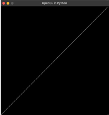
Figure 4.16: The first view from a perspective camera

The reason you are seeing this line across the window is that the cube is being drawn around (0, 0, 0) and the camera is viewing it from (0,0,0). This means the camera is inside the cube and you can only see one side.

3. To get a better view of the cube, the cube needs to be moved into the world along the z axis, like this:

   ..

   white = pygame.Color(255, 255, 255)

   gluPerspective(30, (screen_width / screen_height),

                  0.1, 100.0)

   glTranslatef(0.0, 0.0, -3)

   mesh = Cube()

   ..

Add this line of code and then run HelloMesh again. This time, you will see the entire cube in perspective, as shown in the following screenshot. It doesn’t look like much, but the perspective view allows it to be drawn such that the face of the cube furthest away from the camera appears smaller. glTranslate() adds (0, 0, -3) to each of the cube’s vertices, thus drawing them at a location further away from the camera:

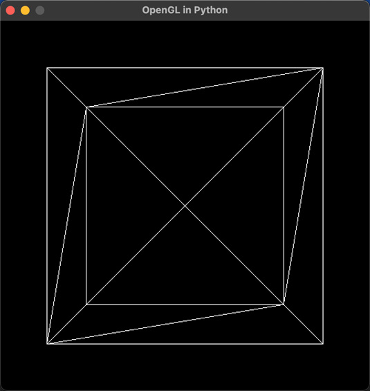
Figure 4.17: A perspective view of a wireframe cube

4. To get a better sense of the 3D nature of the cube, let’s rotate it. Add these lines and then run the application again:

   while not done:

     for event in pygame.event.get():

       ..

     glClear(GL_COLOR_BUFFER_BIT | GL_DEPTH_BUFFER_BIT)

     glRotatef(5, 1, 0, 1)

     mesh.draw()

     pygame.display.flip()

     pygame.time.wait(100);

You’ll now see the cube rotating by 5 around its x axis and 1 around its y axis every 100 milliseconds. At this point, we won’t go into the mechanics of these glRotatef() and glTranslatef() methods as they will be fully explored in later chapters. They are added at this time to help you visualize your drawing better.

5. To change the camera to an orthographic projection, replace the gluPerspective() function with the following:

   glOrtho(-1, 1, 1, -1, 0.1, 100.0)

This call is setting, in order, the left, right, top, and bottom near plane and far plane of the view volume. Note that as the cube rotates when it is perfectly aligned with the camera, the planes line up and for a moment only appear as a square. This is because, in orthographic views, objects are not scaled with distance.

In this section, we have stepped through the mathematics behind graphics projection to transform the vertices of a model into screen coordinates for pixels.

Your turn…

Exercise C: Set up a perspective camera to view the cube with a FOV of 60 with the other parameters remaining as previously used. What do you notice about the drawing between FOV = 30 and FOV = 60?

Summary

In this chapter, we’ve taken a bit of time to focus on how rendering is performed and examined the rendering pipeline and camera setups. A thorough understanding of how these affect the positions and projections of objects in the environment is critical to your understanding of the structure of a 3D environment and the relative locations of drawn artifacts. In addition, considerable time has been spent on elucidating the calculations involved in taking a world vertex position and projecting it onto the screen. The process is not as straightforward as it might first seem, but with a knowledge of basic trigonometry and mathematics, the formulae have been derived.

One common issue that I find when developing these types of applications is just knowing how to debug the code when it seems to be running without syntax errors but nothing appears on the screen. Most often, the issue is that the camera cannot see the object. Therefore, if you can visualize in your mind where the camera is, in which direction it is facing, and whether or not an object is inside the viewing volume, this is a great skill to have.

Another element that assists with visualization in computer graphics is color. This is used from the most basic of drawings, even if they are in black and white, to complex textured surfaces and lighting effects. In the next chapter, we will take a look at the fundamentals of color and how to apply it in computer graphics through code.

Answers

Exercise A:

This is one set of vertices and triangles to draw a cube placed in a new class (note that you might have them in a different order from what is shown here):

from Mesh3D import *
class Cube(Mesh3D):
def __init__(self):
            self.vertices = [(0.5, -0.5, 0.5),
(-0.5, -0.5, 0.5), (0.5, 0.5, 0.5),
(-0.5, 0.5, 0.5),(0.5, 0.5, -0.5),
(-0.5, 0.5, -0.5), (0.5, -0.5, -0.5), (-0.5, -0.5, -0.5),
(0.5, 0.5, 0.5), (-0.5, 0.5, 0.5), (0.5, 0.5, -0.5),
(-0.5, 0.5, -0.5), (0.5, -0.5, -0.5), (0.5, -0.5, 0.5),
(-0.5, -0.5, 0.5), (-0.5, -0.5, -0.5), (-0.5, -0.5, 0.5),
(-0.5, 0.5, 0.5), (-0.5, 0.5, -0.5), (-0.5, -0.5, -0.5),
(0.5, -0.5, -0.5), (0.5, 0.5, -0.5), (0.5, 0.5, 0.5),
(0.5, -0.5, 0.5)
]
          self.triangles = [0, 2, 3, 0, 3, 1, 8, 4, 5, 8,
  5, 9, 10, 6,
  7, 10,
  7, 11, 12, 13, 14,
  12, 14, 15, 16, 17, 18, 16,
  18, 19, 20, 21, 22, 20, 22, 23]

To use this class in HelloMesh.py, include from Cube import * and replace mesh = Mesh3D() with mesh = Cube().

Because of the point of view, the drawing will look the same as the single square because the other sides of the cube are on top of each other.

Exercise B:

Given horizontal_fov = 80, N = 2, screen.width = 1366, and screen.height = 768, this is the result:

vertical_fov = 80 * screen.height/screen.width = 45
right = tan(80/2) * 2 = 1.68
bottom = -tan(45/2) * 2 = -0.83

Exercise C:

The greater the FOV, the more the object is scaled, as illustrated here:

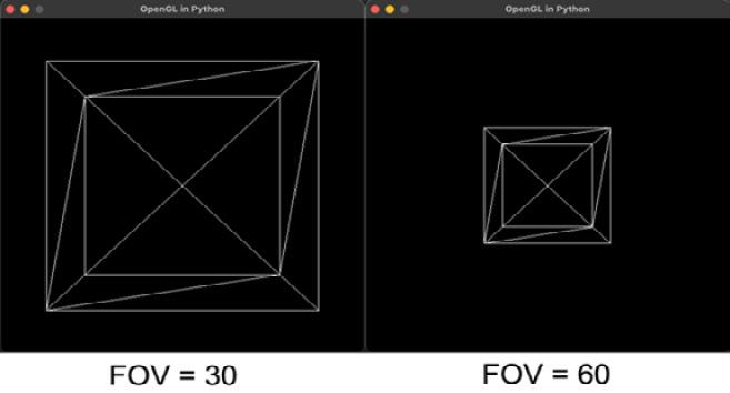
Figure 4.18: A wireframe cube presented with differing FOVs