8

Reviewing Our Knowledge of Triangles

If there’s one area of mathematics that you want to focus on during your educational journey through graphics and games programming, make sure it is vector mathematics. I cannot stress enough how important having a thorough knowledge of this area is to your success in developing your skills in this domain. Trigonometry, which examines the relationships between side lengths and angles in triangles, underpins many of the vector functions. As such, we will be exploring the magic of triangles herein.

Initially, for me, vectors and triangles were taught as separate ideas. It wasn’t until I started using vectors in my game programming that it suddenly became clear how understanding triangles was such a big part of understanding vectors. Also, vectors are just an extension of the mathematics of triangles.

Triangles would have to be one of the most interesting and useful geometrical shapes. Mathematically, their properties are fundamental to understanding a great proportion of the mathematics in graphics, including vectors, distances, and angles. They are used almost everywhere in defining the geometry of 2D and 3D space and the movement within.

Therefore, to ensure you get the best coverage of all the essential components in this chapter, we will cover the mathematics of similar and right-angled triangles. We will explore the following topics:

• Comparing similar triangles
• Working with right-angled triangles
• Calculating angles with sine, cosine, and tangent
• Investigating triangles by drawing 3D objects

By the end of this chapter, you will have developed the skills to apply your knowledge of triangles to problem-solving in numerous geometric situations, in addition to loading a triangle-based mesh file into your project.

We will begin exploring these topics by looking at the mathematical properties of triangles. To do this, we will examine the properties of similar triangles that underpin the geometry that was used in the projections we explored in Chapter 4, Graphics and Game Engine Components.

Technical requirements

The solution files containing the code for this chapter can be found on GitHub at https://github.com/PacktPublishing/Mathematics-for-Game-Programming-and-Computer-Graphics/tree/main/Chapter08 in the Chapter08 folder.

For the practical exercise in this chapter, you will require the teapot.obj model file, which can be downloaded from https://github.com/PacktPublishing/Mathematics-for-Game-Programming-and-Computer-Graphics/tree/main/Chapter08/resources.

Comparing similar triangles

Two triangles are similar when the only difference is the scale, as shown in Figure 8.1, where Triangle (b) is a scaled-down version of Triangle (a):

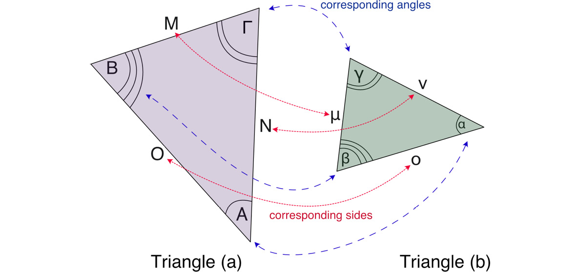
Figure 8.1: Similar triangles

Two triangles are considered similar if they contain the same set of three corner angles. For example, if the angles (in degrees) of Triangle (a) are 60, 45, and 75, then the angles of Triangle (b) must also be 60, 45, and 75. The total of all angles in a triangle equates to 180 degrees.

For similar triangles, the following applies:

• All corresponding angles are equal
• All corresponding sides have the same ratio
• Corresponding sides have the same ratio between them

As triangles are only considered similar if the respective angles are the same between them, as previously discussed. Given Figure 8.1, A = α, B = β, and Γ = γ.

Because, with similar triangles, one is smaller than the other, the ratio of the corresponding sides is the same. For example, in Figure 8.1, we have the following:

If Triangle (b) is half the size of Triangle (a), then we get the following formula:

This is obvious as you would expect that something halved in size would have half the original dimensions.

Let’s take a look at an example. Given the triangles in Figure 8.2, to calculate the missing length of Triangle (c), first, you need to determine whether both Triangle (c) and Triangle (d) are similar. In this case, they are similar as they have the same set of angles:

Figure 8.2: Calculating the missing side

Next, you need to determine what the ratio is between the corresponding sides of Triangle (c) and Triangle (d). Both given sides of Triangle (c) have lengths of 12. Their corresponding sides in Triangle (d), the ones on either side of the 120-degree angle, are 3. Therefore, the ratio is 12:3 or 12/3, which equates to 4. We know from similar triangles that the length of the missing side of Triangle (c) will give a value of 4 when divided by its corresponding side in Triangle (d), which is 6:

Therefore, the length of the missing side is 24.

The same types of comparisons can be used to determine missing angles. Let’s take a look at the example in Figure 8.3. Here, we can see that there are two triangles with missing angles and sides:

Figure 8.3: Calculating multiple values for similar triangles

How can you tell they are similar? Well, you can’t from the information provided, though you could measure the sides and angles to establish that they are similar. But for now, just take my word for it. If you take a look at the side of Triangle (f), which has a length of 5.9, and its location relative to the angle of 110, then you’ll be able to determine its corresponding side in Triangle (e), which is the side with a length of 11.8. In this case, the ratio is 11.8/5.9, which equals 2. This tells you that Triangle (e) is twice the size of Triangle (f). Given this information, you can calculate the length of A like so:

To determine the length of B in Triangle (e), you can use the following calculation:

Finally, there are the missing angles, which are labeled C, D, and E. We can determine angle E as we know that there are 180 degrees in a triangle. So, by subtracting the angles we have in Triangle (e), we can determine the following:

Because the corresponding angles in Triangle (f) will have the same value in degrees as Triangle (e), D will be 30 and E will be 40.

Now, let’s put your newfound skills in dealing with similar triangles to use.

Your turn…

Exercise A. Are the triangles in Figure 8.4 similar? If so, find the value of angle J in Triangle (g) and the value of angle K in Triangle (h):

Figure 8.4: Are these similar?

The third observation regarding similar triangles is that the ratios between sides are the same. This means that if you take two sides with the same angle between them in Triangle (g) and the corresponding sides in Triangle (h), then their ratios will be equal.

With that, you’ve learned how similar triangles work and how useful this knowledge was for calculating project spaces in Chapter 4, Graphics and Game Engine Components. For these particular calculations, we also took advantage of the properties of a special subset of triangles in which one angle is 90 degrees. These, as you will already know, are called right-angled triangles, and understanding them will form the basis for your appreciation of vectors later in this chapter.

Working with right-angled triangles

Since mathematics in grade school, we’ve learned about Pythagoras. He was the Greek mathematician who came up with the relationship between the lengths of the sides of a right-angled triangle. This relationship is so important to vector mathematics that it is worth learning it off by heart. It states that for a right-angled triangle, the square of the hypotenuse (the longest side) is equal to the sum of the squares of the other two sides. Such a triangle is illustrated in Figure 8.5, with c indicating the hypotenuse:

Figure 8.5: A right-angled triangle

Given the right-angled triangle in Figure 8.5, the relationship between the hypotenuse and other sides can be written like this:

Important note

The hypotenuse is the side opposite the right angle.

Let’s work through the calculation of the hypotenuse using the triangle in Figure 8.6:

Figure 8.6: A right-angled triangle (with the length of two sides given)

Here, we can see the lengths of two sides of the triangle. With respect to the triangle in Figure 8.5, a = 4 and b = 3. To calculate the length of the hypotenuse (c), we must perform the following operations:

The same formulae can be used to determine the length of a side if the hypotenuse and one side are given (provided you are certain the triangle does indeed have a right angle). Given Triangle (i) in Figure 8.7, to calculate the side indicated by x, we would perform the following:

Figure 8.7: Right-angled triangles with a hypotenuse length and one side length

Now, it’s your turn to test your knowledge of right-angled triangles.

Your turn…

Exercise B. Calculate the value of x for Triangle (j) and Triangle (k) in Figure 8.7.

The hypotenuse of a right-angled triangle, as you will see in Chapter 9, Practicing Vector Essentials, represents the body of a vector and it is our new skill in calculating the length of a hypotenuse that will be used over and over again in vector mathematics.

Besides being able to calculate the lengths of the sides of a right-angle triangle by using Pythagoras’ theorem, we can also use the value of the angles of the triangle to calculate the same values.

Calculating angles with sine, cosine, and tangent

The length of the hypotenuse and the other two sides can be determined using the triangle’s angles and the sine, cosine, and tangent operations. The sides of a right-angled triangle, apart from the hypotenuse, can be labeled as Opposite and Adjacent based on their positions in the triangle relative to the relevant angle, as shown in Figure 8.8:

Figure 8.8: The adjacent and opposite triangle sides for

Note that for these rules, either angle can be used. If the angle at the other end of the hypotenuse (other than what is shown in Figure 8.8) is used, then the labels for Opposite and Adjacent change positions.

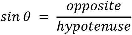
The relationship between the sides and hypotenuse that represent the trigonometric function of sine is as follows:

The relationship for the trigonometric function of cosine is as follows:

The relationship for the trigonometric function of tangent is as follows:

Working with the triangles in Figure 8.5 and Figure 8.6, we can calculate angle Φ given that a = 4 and b = 3. As we have the values for the Opposite and Adjacent sides, we can use the tangent rule:

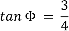
In the preceding calculation, 3 is the length of the side opposite angle Φ and 4 is the length of the adjacent side.

The same calculation can also be calculated with sine:

In this calculation, 3 is the opposite angle and 5 is the hypotenuse. As you may have guessed, we can also perform the same calculation using the cosine method:

Here, because we are now using cosine, the adjacent side of 4 is used instead of the opposite side of 3.

Note that the trigonometric functions work with radians:

You can convert between radians and degrees like so:

tan-1, cos-1, and sin-1 in the previous equations can be calculated using arctan, arccos, and arcsin, respectively, which are the inverse of each function. If you need to calculate any of these values, using Google is an easy way if you don’t have a scientific calculator. For the previous calculation, I found the values by typing arctan(0.75) in degrees into my browser’s search box. The result is shown in Figure 8.9:

Figure 8.9: Using Google to perform calculations

Now, it’s your turn to test your newfound skills in determining the lengths of some triangle sides.

Your turn…

Exercise C. Given the right-angled triangles in Figure 8.10, find the missing angles and sides:

Figure 8.10: Right-angled triangles to test your knowledge of trigonometric functions

Now that you’ve spent time exploring the mathematics of triangles, it’s time to use them in our Python project.

Investigating triangles by drawing 3D objects

Triangles were introduced in our Python/OpenGL project in Chapter 4, Graphics and Game Engine Components, when they were used to define the vertices and surfaces of 3D models. Triangles are the most efficient way to define a surface as they contain only three vertices. This is the minimum number of points required to define a flat plane with two points only able to define a line, which extends from one to the other.

3D meshes defined with triangles are said to be triangulated. While a model can be created by a 3D modeling package with polygons that have more vertices than triangles, software provides artists with a way to triangulate a model so that it can be imported into graphics and game engines. Figure 8.11 shows a triangulated model of a teapot in Autodesk Maya LT and the menu function that will reduce a complex model to triangles:

Figure 8.11: A triangulated teapot in Maya LT

While it is possible to define this teapot model in Python as a manually typed set of vertices, triangles, and UVs, it can be quite laborious to do so. Therefore, before you can explore more complex models in the project we are creating, we should add a simple model loader class.

We will do this by developing a new class that inherits from the Mesh3D class.

Let’s do it...

In this exercise, we will examine the format of the Wavefront OBJ 3D model file and develop a Python class to load a model from a .obj file into our project:

1. Create a new folder in PyCharm called Chapter Eight and make copies for it of the final versions of the files from Chapter Seven. Then, include Button.py, Cube.py, Mesh3D.py, Object.py, Settings.py, Transform.py, and Utils.py. Also, make a copy of AddingButtons.py from Chapter Seven for Chapter Eight but rename it DisplayTeapot.py.
2. In the Chapter Eight folder, create a folder called models and copy the teapot.obj file from GitHub into it.
3. Create a new Python script called LoadMesh.py and add the following code:

   from Mesh3D import *

   class LoadMesh(Mesh3D):

       def __init__(self, draw_type, model_filename):

           self.vertices, self.triangles =

                        self.load_drawing(model_filename)

           self.draw_type = draw_type

       def draw(self):

           for t in range(0, len(self.triangles), 3):

               glBegin(self.draw_type)

               glVertex3fv(self.vertices[

                           self.triangles[t]])

               glVertex3fv(self.vertices[

                           self.triangles[t + 1]])

               glVertex3fv(self.vertices[

                           self.triangles[t + 2]])

               glEnd()

           glDisable(GL_TEXTURE_2D)

The first part of the LoadMesh class declares the vertices and triangles and loads them from a model file that is passed through to the constructor in the form of an external .obj file. This will become the teapot.obj file in the models folder. The draw() method is a copy of that from Mesh3D with the UV values taken out. They aren’t needed initially, so rather than upsetting the existing code in Mesh3D, for now, it’s simpler to just include another copy here:

    def load_drawing(self, filename):
        vertices = []
        triangles = []
        with open(filename) as fp:
            line = fp.readline()
            while line:
                if line[:2] == "v ":
                    vx, vy, vz = [float(value) for
                                  value in
                                  line[2:].split()]
                    vertices.append((vx, vy, vz))
                if line[:2] == "f ":
                    t1, t2, t3 = [value for value in
                                  line[2:].split()]
                    triangles.append(
                       [int(value) for value in
                        t1.split('/')][0] - 1)
                    triangles.append(
                       [int(value) for value in
                        t2.split('/')][0] - 1)
                    triangles.append(
                       [int(value) for value in
                        t3.split('/')][0] - 1)
                line = fp.readline()
        return vertices, triangles

The next method loads in a .obj file that’s looking for the lines starting with 'v ' and 'f '. If you take a look inside the .obj file (you can open it up in PyCharm), you will see that these lines are marked:

v 0.000000 2.400000 -1.400000
v 0.229712 2.400000 -1.381970
v 0.227403 2.435440 -1.368070
f 3176/12689/12754 3156/12690/12755 3157/12691/12756
f 3177/12692/12757 3156/12693/12758 3176/12694/12759
f 3177/12695/12760 3155/12696/12761 3156/12697/12762

The lines beginning with v are vertex positions. All of these lines collectively define the array of vertices for the mesh.

The lines beginning with f are a set of three indices. The first number in each set specifies the indices in the array of vertex values or what you have been referring to thus far as the triangle values. The other two values are for defining uvs and normals (something we will discuss in future chapters).

A full description of the .obj file format can be found at https://en.wikipedia.org/wiki/Wavefront_.obj_file.

4. To load this model into the project, open DisplayTeapot.py and make the following changes:

   import math

   import pygame.mouse

   from Object import *

   from Cube import *

   from LoadMesh import *

   from pygame.locals import *

   …

   objects_2d = []

   cube = Object("Cube")

   cube.add_component(Transform((0, 0, -5)))

   cube.add_component(LoadMesh(GL_LINE_LOOP,

                      "models/teapot.obj"))

   objects_3d.append(cube)

Notice that the code uses the existing cube object and replaces the Cube() class with the LoadMesh() class instead. Now, when you run DisplayTeapot.py, a wireframe teapot will be drawn, as shown in Figure 8.12:

Figure 8.12: A triangulated teapot in Maya LT

The application will run as it did with the cube in Chapter 7, Interactions with the Keyboard and Mouse for Dynamic Graphics Programs. You will be able to move the teapot around with the arrow keys.

The OBJ model loader we have added to our project is very basic, but it demonstrates just how many triangles go into making up a mesh. In addition, having a loading functionality in the project will allow you to experiment with bringing other .obj files in and loading them. Just ensure they have been triangulated. There’s a large variety of other data in the .obj file to be dealt with, and we will address this as we progress through this book.

Summary

An understanding of triangles is essential for those who want to program in the graphics and games domains. They are the foundation of the data structures used to store meshes, as well as the basic drawing components of them. When it comes to mathematics in these realms, they are equally as important. Their trigonometric properties, as you will see in the next chapter, form the basis of vector mathematics.

In this chapter, you explored the fundamental properties of triangles and learned how to calculate the length of a triangle’s sides and angles using the relationships between similar triangles and the trigonometric rules found in right-angled triangles. Following the theory, we applied our knowledge of triangles to load a triangulated mesh into OpenGL and display it.

Now that you have explored the mathematics of triangles, we can start examining vectors.

Answers

Exercise A:

These two triangles are similar. You only need two corresponding angles and two corresponding sides to determine this fact. Both triangles have angles of 60 and 75. This is enough to establish that the triangles are similar because if you take 60 and 75 away from 180 (the total of the angles in a triangle), then the remaining angle of K for Triangle (h) will be 45 and the corresponding angle in Triangle (g) will also be 45.

To find the length of J, you need to establish the ratio of the other corresponding sides. As the triangles are similar, you will know that the known two sides will have the same ratio – that is, 3/2 = 2.8/1.86 = 1.5.

Using this ratio, we can calculate J to be 4.8/1.5 = 3.2.

Exercise B:

This is the value of x in Triangle (j):

This is the value of x in Triangle (k):

Exercise C:

(X) To find θ, we must use the cosine rule, which, when written as a Google search, becomes arccos(5/7) in degrees, which is 44.42. To find the value of a, now that we have a value for θ, we can use the sine rule:

The Google search that we used here is . Note that the value given to the sine function must be in radians, but since we have calculated the angle in degrees, I’ve simply informed Google that the angle I am giving the sine function is in degrees.

(Y) To find θ, we must use the sine function so that we get arcsin(8/10) in degrees, which gives us 53.13. So, the value of a can be found with the cosine rule:

(Z) To find a, we can use the cosine rule:

To find b, once we have the value of a, we can use the tan rule:

Alternatively, we can use the sine rule: