
11
Manipulating the Light and Texture of Triangles
We started drawing triangles back in Chapter 2, Let’s Start Drawing, and added lighting and texturing in Chapter 5, Let’s Light It Up! Now that we’ve covered normals in Chapter 10, Getting Acquainted with Lines, Rays, and Normals, it’s time to put it all together to take a look at how these special vectors are used to manipulate and affect the appearance of triangles.
Normals can belong to vertices and mesh faces. Besides being used to specify which side of a polygon should be rendered, they are also used to calculate how light falls across the surface of a polygon. In this chapter, we will begin by improving on the normal drawing technique discussed in Chapter 10, Getting Acquainted with Lines, Rays, and Normals, and use more vector calculations on triangles to find the center of a triangle and draw the normal from that point. This will allow you to draw normals on any mesh in your project, not just cubes. Following this, you will examine how OpenGL uses normals to define the side of a polygon on which a texture will be displayed. In addition, we will explore some special uses of normals in determining whether only one side or both sides of a polygon should be displayed depending on the object that requires rendering. After this, we will delve back into the process of lighting a scene and examine the effect normals have on how light falls across the surface of a polygon.
In this chapter, you will build on your skills in rendering and understanding the nature of 3D model surfaces through the following topics:
- Displaying Mesh Triangle Normals
- Defining Polygon Sides with Normals
- Culling Polygons According to the Normals
- Exploring How Normals Affect Lighting
By the end of this chapter, you will have developed the practical skills to control which sides of a polygon you require to be lit and textured.
Technical requirements
In this chapter, we will continue to work on the project being constructed in Python, PyCharm, Pygame, and PyOpenGL.
The solution files containing the code can be found on GitHub at https://github.com/PacktPublishing/Mathematics-for-Game-Programming-and-Computer-Graphics/tree/main/Chapter11in the Chapter11 folder.
Displaying Mesh Triangle Normals
We will begin this chapter by adding some extra functionality to the normal drawing in Chapter 10, Getting Acquainted with Lines, Rays, and Normals. At the time, we restricted the drawing of these normals to the center of the cube being drawn. This technique won’t work with more complicated meshes. More ideally, it would work better if each normal for a plane were emitted from the center point of the triangle, which is called the centroid. The centroid can be found using the medians of the vectors that make up its sides. Take, for example, the triangle in Figure 11.1:

Figure 11.1: The centroid of a triangle
The centroid can be found by finding a point halfway along any of the sides, connecting that point with the opposite corner, and then moving along the vector from the corner to the halfway point by two-thirds. In this example, that means if you find the vector from corner A to B and then travel halfway along it to locate point D, the centroid will be two-thirds of the way along the vector connecting C to D. This is true of the simple calculation made on any of the three sides and their opposite corners.
We will start the practical exercises in this chapter by relocating the starting position of the normals drawn at the end of Chapter 10, Getting Acquainted with Lines, Rays, and Normals.
Let’s do it…
In this exercise, we will adjust the starting point of the DisplayNormals class to allow for the visualization of the normals on any mesh:
- Begin by making an exact copy of your project folder as it was at the very end of Chapter 10, Getting Acquainted with Lines, Rays, and Normals. Name the copied folder Chapter 11.
- Modify the code in DisplayNormals.py to calculate and use the median of each triangle like this:
…
for t in range(0, len(self.triangles), 3):
vertex1 = self.vertices[self.triangles[t]]
vertex2 = self.vertices[self.triangles[t + 1]]
vertex3 = self.vertices[self.triangles[t + 2]]
p = pygame.Vector3(vertex1[0] - vertex2[0],
vertex1[1] - vertex2[1],
vertex1[2] - vertex2[2])
q = pygame.Vector3(vertex2[0] - vertex3[0],
vertex2[1] - vertex3[1],
vertex2[2] - vertex3[2])
norm = cross_product(p, q)
#find median
midpoint = vertex3 + q * 0.5
v = (midpoint - vertex1) * 2/3
centroid = vertex1 + v
self.normals.append((centroid, centroid + norm))
In this code, the midpoint between vertex2 and vertex3 is calculated by adding half of the vector between the points to vertex3. A vector between this midpoint and the opposite corner of vertex1 is calculated and two-thirds of this is used to add to vertex1.
Important note
You could use any combination of corners and sides using the same rules to find the centroid. This centroid point is then used as the starting position for the normal.
- Run the Animate.py file that has been copied to the Chapter 11 folder to see the result. Note the new starting position for the normals, as shown in Figure 11.2 (with a little embellishment to make it obvious):

Figure 11.2: A closeup of the normals drawn for each cube triangle
Having made these changes, you will now be able to draw any mesh and display the normals.
- To have a look at the normals on a mesh loaded from a file, make a copy of Animate.py and rename it ExploreNormals.py.
- Download a copy of planesm.obj from the Chapter 11/models folder on GitHub and place this file in PyCharm in the Chapter 11/models folder.
- From GitHub, download a copy of ExploreNormals.py from the Chapter11/startercode folder and replace your code with the code in this new file. This code will replace all the cube and grid drawings, as well as the animations with a wireframe view of planesm.obj. But don’t run it yet as we need to make a few more adjustments to get the code to execute correctly.
- The plane you are about to draw is facing the camera. This will make it difficult to see the normals. Therefore, we can temporarily rotate and recolor it by changing the code in Object.py like this:
def update(self, events = None):
glPushMatrix()
for c in self.components:
if isinstance(c, Transform):
pos = c.get_position()
glTranslatef(pos.x, pos.y, pos.z)
glRotate(45, 0, 1, 0)
elif isinstance(c, Mesh3D):
glColor(1, 1, 1)
c.draw()
elif isinstance(c, Grid):
c.draw()
These new lines will rotate the plane by 45 degrees around the y- axis and recolor the polygon wireframe to draw in white.
- One last change to make before running ExploreNormals.py is to increase the length of the normals to make them visible. We can do this in DisplayNormals.py by adding a multiplier to the end position of the normals, as follows:
middle = (vertex3 + q * 0.5)
v = (middle - vertex1) * 2/3
median = vertex1 + v
nstart = median
self.normals.append((nstart, nstart + norm * 10))
By multiplying the normal (which has a length of 1) by 10, it will make them go in the same direction but display a longer-drawn line.
- Now it’s time to play ExploreNormals.py. When you do, you will see the mesh in white and normals in green, as shown in Figure 11.3:

Figure 11.3: Displaying normals on a loaded mesh
Note how each of the normals is drawn from the centroid of each triangle. As was the case with the previous normal calculations in step 2, we determined them from the triangle vertices, where the vertices for each triangle were all listed in anticlockwise order.
While the normals included in the .obj file face in one direction, mathematically they can face in either direction at 90 degrees to the plane. The effects of this on drawing will now be explored.
Defining polygon sides with normals
So far in this book, we’ve calculated normals but not explored their many uses. One of these uses is to dictate which side of a polygon is visible. The same plane that you have been using up to this point has had the normals reversed in Autodesk Maya, a 3D modeling program, for the center polygons, as shown in Figure 11.4:

Figure 11.4: A plane with some normals reversed
The black section in the middle of the plane in Figure 11.4 when rendered would in fact appear as a hole when viewed from one direction and solid from the other. Even though it might look like a hole, that doesn’t mean there aren’t any polygons covering this area. When this plane is drawn with a cube behind it in Python and OpenGL, the hole is evident, as shown in Figure 11.5 (a):
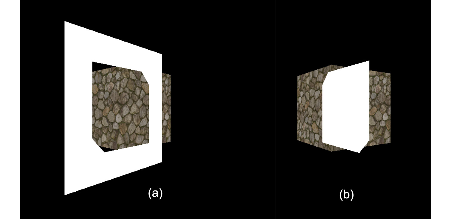
Figure 11.5: A plane with normals reversed viewed from both sides
As can be seen in Figure 11.5, whichever polygons have normals on the same side of the camera are opaque. Figure 11.5 (a) is a view from the front and Figure 11.5 (b) is when the scene is rotated by 180 degrees. What appears as a hole in Figure 11.5 (a) can be seen as polygons in Figure 11.5 (b).
In some cases, you’ll want to be able to see polygons on just one side, and in others on both sides. In the next section, we will explore these cases.
Working with visible sides of a polygon
Why would we want the option of enabling or disabling the visible sides of polygons? There are two popular cases.
The most common use of a single plane is when it needs to represent something solid. A plane has no thickness mathematically. However, using a box or other 3D shape when only a very thin flat surface is required more than doubles the number of polygons needed to draw the object because a flat plane only has one surface, whereas a cube has six. For example, if you are modeling the interior of a sci-fi corridor, each wall panel, as shown in Figure 11.6, only needs to be a single plane with an image on one side:

Figure 11.6: Wall panels represented by a single plane
If the player or viewer is never going to see the plane from the other side, then it is a waste of memory and processing effort to try and render it.
The next most common use of a plane to represent something solid is when you need to see a flat plane from both sides, as is the case with leaves. There can be hundreds or even millions of these in a graphics or game environment. The most memory-efficient way of drawing a leaf is with a flat plane displaying the texture, as shown in Figure 11.7:
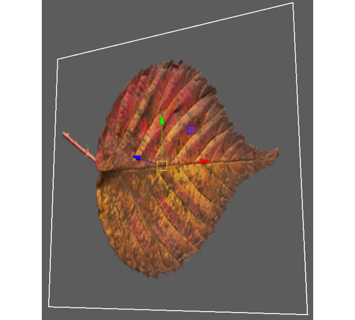
Figure 11.7: A leaf image on a plane
This texture needs to be visible from both sides because you don’t want to duplicate the geometry or leaf texture to make it visible on both sides. A plane that is visible on both sides is called a billboard. It is used for a variety of purposes, such as faking distant geometry and buildings or for individual leaves and branches on vegetation and grass. Because it is flat, the illusion of 3D that a billboard is attempting to fake will be lost depending on the viewing direction.
Figure 11.8 (a) shows a tree that would be acceptable to a viewer from the ground level, but when viewed from above (Figure 11.8 (b)), the illusion is broken and the flat nature of the leaves is noticeable:
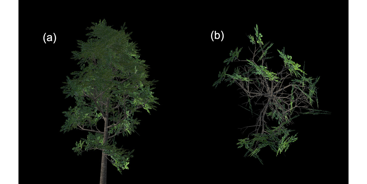
Figure 11.8: Branch billboards from different points of view
However, when you want to generate and display an entire forest in 3D, it’s in no way practical to accurately model and render individual leaves.
In the next section, you will discover how you can enable and disable the drawing of polygon sides based on their normals.
Culling Polygons According to the Normals
The removal of a polygon from rendering is called culling. Culling can occur on an entire polygon or just one side. The side that is removed during the culling process is called the backface and it is the opposite side of the polygon to that from which the normal is projected.
In the next practical exercise, we will explore how normals are used to display these types of images.
Let’s do it…
So far, the polygons we have been rendering have had textures on both sides, unbeknownst to you. Now it’s time to take a look at what’s going on both sides:
- From GitHub, download a copy of plane2.obj from the Chapter 11/models folder and place it in your project’s model folder.
- Make the following changes to ExploreNormals.py:
from Cube import *
..
objects_3d = []
objects_2d = []
cube = Object("Cube")cube.add_component(Transform((0, 0, -3)))
cube.add_component(Cube(GL_POLYGON,
"images/wall.tif"))
mesh = Object("Plane")mesh.add_component(Transform((0, 0, -1.5)))
mesh.add_component(LoadMesh(GL_TRIANGLES,
"models/plane2.obj"))
objects_3d.append(cube)
objects_3d.append(mesh)
The first part of the new code places the textured cube back in the scene. If you’ve used a different image file to texture your cube, then ensure you use the filename for your texture instead of wall.tif.
Other changes have been made to the loading of the mesh to make it draw using GL_TRIANGLES instead of GL_LINE_LOOP. A new plane model is being used. This model is the one with the apparent hole in it that we saw in Figure 11.5.
Also, be sure to remove the DisplayNormals component we used on the mesh and cube in the previous exercise.
- We will now modify the drawing of these 3D objects by allowing them to rotate, and thus allow us to view both sides. To do this, open up the Object.py script and make the following changes:
class Object:
def __init__(self, obj_name):
self.name = obj_name
self.components = []
self.scene_angle = 0
..
def update(self, events = None):
glPushMatrix()
for c in self.components:
if isinstance(c, Transform):
pos = c.get_position()
glTranslatef(pos.x, pos.y, pos.z)
self.scene_angle += 0.5
glRotate(self.scene_angle, 0, 1, 0)
elif isinstance(c, Mesh3D):
This will keep track of a scene_angle value used to set the viewing angle. By updating the value of this variable in the update method, we can constantly rotate the scene.
- Run ExploreNormals.py to watch the plane and cube rotating. The plane will look like a square colored entirely in white, as shown in Figure 11.9, with the textured cube behind it:
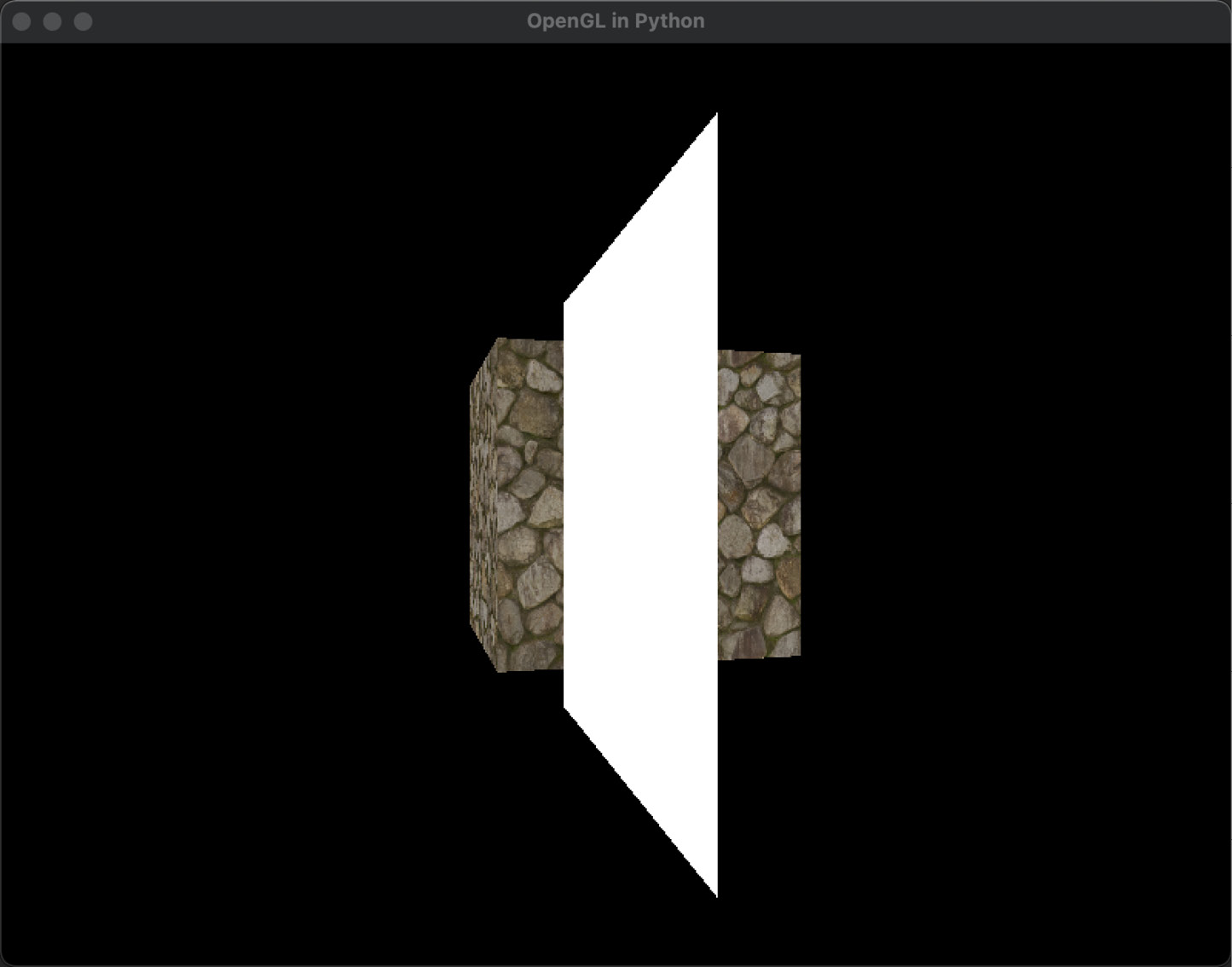
Figure 11.9: A rotating cube behind a white plane
Believe it or not, this plane has the normals in the center reversed like the one in Figure 11.5. The reason you can’t see the hole or reversal of normals is that by default, OpenGL is drawing both sides of the plane.
- To only display the side of each polygon from which the normals emanate, edit the set_3d method in ExploreNormals.py to include the following:
..
def set_3d():
glMatrixMode(GL_PROJECTION)
..
glViewport(0, 0, screen.get_width(),
screen.get_height())
glEnable(GL_DEPTH_TEST)
glEnable(GL_CULL_FACE)
while not done:
events = pygame.event.get()
..
The GL_CULL_FACE directive tells OpenGL to ignore drawing the backface of polygons.
- Run ExploreNormals.py again to see the plane drawing with the normals reversed in the middle, as shown in Figure 11.5.
The GL_CULL_FACE setting is OpenGL’s command to prevent the reverse side of polygons from being drawn. This process is called backface culling. This dramatically increases performance as it cuts down how many polygons in a scene get rendered. It can be turned on with glEnable(GL_CULL_FACE) and turned off with glDisable(GL_CULL_FACE), so the programmer can control which meshes draw on both sides and which don’t. We will demonstrate this in the next exercise.
Let’s do it…
As previously discussed in the Working with visible sides of a polygon section, one type of mesh that would require both sides to be drawn is for leaves. In this exercise, we will add this object, and you will learn how to turn backface culling on and off:
- Before we can show both sides of a mesh being drawn with a texture, the LoadMesh class needs to be updated to accommodate the addition of a texture. Much of this code should be familiar to you from the Mesh3D class. Open LoadMesh.py and make the following changes:
class LoadMesh(Mesh3D):
def __init__(self, draw_type, model_filename,
texture_file=""):
self.vertices, self.uvs, self.triangles =
self.load_drawing(model_filename)
self.texture_file = texture_file
self.draw_type = draw_type
if self.texture_file != "":
self.texture =
pygame.image.load(texture_file)
self.texID = glGenTextures(1)
textureData = pygame.image.tostring(
self.texture, "RGB", 1)
width = self.texture.get_width()
height = self.texture.get_height()
glBindTexture(GL_TEXTURE_2D, self.texID)
glTexParameteri(GL_TEXTURE_2D,
GL_TEXTURE_MIN_FILTER,
GL_LINEAR)
glTexImage2D(GL_TEXTURE_2D, 0, 3, width,
height,
0, GL_RGB, GL_UNSIGNED_BYTE,
textureData)
The first changes to the code made in the __init__ method test to see whether a texture filename has been passed through. If it has, then the same code used in Mesh3D.py to load in a texture and initialize the required parameters is included.
The next changes occur in the draw method of LoadMesh.py:
    def draw(self):
        if self.texture_file != "":
            glEnable(GL_TEXTURE_2D)
            glTexEnvf(GL_TEXTURE_ENV,
                      GL_TEXTURE_ENV_MODE,
                      GL_DECAL)
            glBindTexture(GL_TEXTURE_2D, self.texID)
        for t in range(0, len(self.triangles), 3):
            glBegin(self.draw_type)
            if self.texture_file != "":
                glTexCoord2fv(
                     self.uvs[self.triangles[t]])
            glVertex3fv(
                self.vertices[self.triangles[t]])
            if self.texture_file != "":
                glTexCoord2fv(
                    self.uvs[self.triangles[t + 1]])
            glVertex3fv(self.vertices[self.triangles[t
                        + 1]])
            if self.texture_file != "":
                glTexCoord2fv(
                    self.uvs[self.triangles[t + 2]])
            glVertex3fv(self.vertices[self.triangles[t
                        + 2]])
            glEnd()
        if self.texture_file != "":
            glDisable(GL_TEXTURE_2D)
Within the draw method, the texture drawing is enabled if there is a texture file. If there’s no texture filename given to the class, the mesh draws as it did before, without a texture and in white.
As we are now using a texture, uvs values must be included with the drawing of each vertex, and so checks for the texture file are performed again before the uvs values are used:
    def load_drawing(self, filename):
        vertices = []
        uvs = []
        triangles = []
        with open(filename) as fp:
            line = fp.readline()
            while line:
                if line[:2] == "v ":
                    ..
                if line[:2] == "vt":
                    vx, vy = [float(value) for value
                              in line[3:].split()]
                    uvs.append((vx, vy))
                if line[:2] == "f ":
                    ..
                line = fp.readline()
        return vertices, uvs, triangles
Lastly, the load_drawing method is expanded to read in the lines from the OBJ file that contain the uvs values. This is a nice feature as it saves us from typing them in manually.
- ExploreNormals.py can now be changed to draw two planes and a cube. We will draw both the previous plane without a hole and the one with the hole. The plane without the hole will be textured. Be sure to use your own texture file in place of the one I have used:
objects_2d = []
cube = Object("Cube")cube.add_component(Transform((0, 0, -3)))
cube.add_component(Cube(GL_POLYGON,
"images/wall.tif"))
mesh = Object("Plane")mesh.add_component(Transform((-1.5, 0, -3.5)))
mesh.add_component(LoadMesh(GL_TRIANGLES,
"models/plane2.obj"))
leaf = Object("Leaf")leaf.add_component(Transform((0.5, 0, -1.5)))
leaf.add_component(LoadMesh(GL_TRIANGLES,
"models/plane.obj",
"images/brick.tif"))
objects_3d.append(cube)
objects_3d.append(mesh)
objects_3d.append(leaf)
clock = pygame.time.Clock()
Here, you can see the drawing will have a cube and two planes. Be sure to change the positions of each via its transform values to ensure they are all visible in the drawing.
Finally, comment out or remove the GL_CULL_FACE enabling:
def set_3d():
    glMatrixMode(GL_PROJECTION)
    ..
    glEnable(GL_DEPTH_TEST)
    #glEnable(GL_CULL_FACE)
Run ExploreNormals.py and note how the backfaces of all drawn polygons are visible, as shown in Figure 11.10:

Figure 11.10: Drawing without culling backface polygons
- Edit LoadMesh.py and modify the code to accept a parameter to enable back_face_cull like this:
class LoadMesh(Mesh3D):
def __init__(self, draw_type, model_filename,
texture_file="", back_face_cull=False):
..
self.draw_type = draw_type
self.back_face_cull = back_face_cull
First, an optional parameter for the LoadMesh class is passed through from where the class is being instantiated. Then, in the draw method, the same parameter is used to turn backface culling on and off:
def draw(self):
    if self.back_face_cull:
        glEnable(GL_CULL_FACE)
    if self.texture_file != "":
        glEnable(GL_TEXTURE_2D)
        ..
    if self.texture_file != "":
        glDisable(GL_TEXTURE_2D)
    if self.back_face_cull:
glDisable(GL_CULL_FACE)- Lastly, we will have the plane with the hole in it, using backface culling. To do this, modify its creation code in ExploreNormals.py, as follows:
mesh = Object("Plane")mesh.add_component(Transform((-1.5, 0, -3.5)))
mesh.add_component(LoadMesh(GL_TRIANGLES,
"models/plane2.obj",
back_face_cull=True))
- Now, when you run ExploreNormals.py, the plane containing the hole will draw only the sides of the polygons with the normals. The other plane will look the same on both sides, as shown in Figure 11.11:
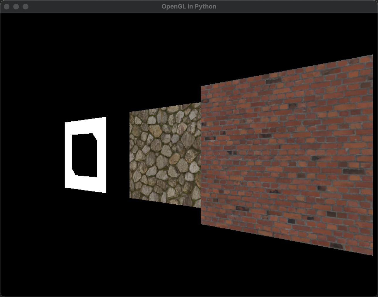
Figure 11.11: Drawing only one mesh with backface culling
In this section, you have learned how to pull in the normals from an OBJ mesh file and use them to control the sides of a polygon that are rendered. This is a valuable skill in learning how to optimize the drawing speed of 3D scenes by eliminating the sides that don’t need to be processed.
Normals are not only used to determine the front and backfaces of polygons but are also essential in calculating lighting effects. A preliminary exploration of normals and lights will be presented next.
Exploring How Normals Affect Lighting
Lighting is a complex topic in graphics. So far, we’ve applied very simple ambient and diffuse lighting to a cube in Chapter 5, Let’s Light It Up! At the time, we discussed the lighting model of specular reflection but didn’t practically apply it as it requires the use of normals. For your convenience, Figure 5.2 of Chapter 5, Let’s Light It Up!, is repeated here as Figure 11.12:

Figure 11.12: The components of light that make up a final render
For ambient and diffuse lighting, the normal is not used and as such makes the surface of meshes appear flat with very little indication of the direction of the light source. To add specular lighting though, we need to know the normal.
Although we didn’t specify the normals for the cube in the light exercise in Chapter 5, Let’s Light It Up!, we were still able to get a lighting effect. However, this lighting was incorrect, as you will see in the next exercise. When OpenGL doesn’t receive any information about normals, it calculates its own by assuming the vertices for triangles are given to it in counter-clockwise order. However, unless we specify the order of vertices ourselves, we can’t be sure they are in counter-clockwise order, especially when an external file format such as OBJ is being used.
In the following exercise, we will take a quick look at the effect of lighting and adding normals, while leaving the hardcore lighting applications and discussion for Chapter 18, Customizing the Render Pipeline.
Let’s do it…
In this practical exercise, we are going to add light to a scene and compare OpenGL’s normal calculations to our own:
- Create a new Python script called NormalLights.py.
- Copy the code from ExploreNormals.py into NormalLights.py.
- Download a copy of cube.obj in the models folder from Chapter 11 on GitHub. This file contains normal values for a cube model.
- Place cube.obj into your models folder for the current project.
- Modify NormalLights.py to turn on some lights by adding the following code to the set_3d() method:
def set_3d():
glMatrixMode(GL_PROJECTION)
glLoadIdentity()
gluPerspective(60, (screen_width / screen_height),
0.1,
100.0)
glMatrixMode(GL_MODELVIEW)
glLoadIdentity()
glViewport(0, 0, screen.get_width(),
screen.get_height())
glEnable(GL_DEPTH_TEST)
glEnable(GL_LIGHTING)
glLight(GL_LIGHT0, GL_POSITION, (5, 5, 5, 0))
glLightfv(GL_LIGHT0, GL_AMBIENT, (1, 0, 1, 1))
glLightfv(GL_LIGHT0, GL_DIFFUSE, (1, 1, 0, 1))
glLightfv(GL_LIGHT0, GL_SPECULAR, (0, 1, 0, 1))
glEnable(GL_LIGHT0)
This code is the same code we used in Chapter 5, Let’s Light It Up! It enables lighting, positions a light at (5, 5, 5, 0), and then specifies the colors for the ambient, diffuse, and specular lights, before enabling the only light in the scene.
- Reduce the number of objects being drawn in the scene by having just one that draws a cube from the cube.obj file by modifying NormalLights.py like this:
..
objects_3d = []
objects_2d = []
cube = Object("Cube")cube.add_component(Transform((0, 0, -3)))
cube.add_component(LoadMesh(GL_TRIANGLES,
"models/cube.obj"))
objects_3d.append(cube)
clock = pygame.time.Clock()
fps = 30
..
- Press play to see a single cube rotating in the scene. Take note of how it changes color. It seems to randomly change from yellow to purple without giving any indication of the direction of the light source that we placed at (5, 5, 5), as shown in Figure 11.13:

Figure 11.13: The components of light that make up a final render
Whatever normal values OpenGL is calculating are wrong. The cube should appear to be lit from a single direction. In addition, OpenGL is only using one normal per triangle face instead of a normal for each vertex.
- We will now modify LoadMesh.py to load the normals out of the OBJ file, as follows:
class LoadMesh(Mesh3D):
def __init__(self, draw_type, model_filename,
texture_file="",
back_face_cull=False):
self.vertices, self.uvs, self.normals,
self.normal_ind, self.triangles =
self.load_drawing(model_filename)
self.texture_file = texture_file
In this code, we are going to get a set of normals and a set of normal indices returned from the loading of the mesh. The indices for the normals act in the same way as the triangles do for the vertices to make sure they are used in the correct order.
- Continue to edit LoadMesh.py to load in the normals and normal indices from the OBJ file like this:
..
def load_drawing(self, filename):
vertices = []
uvs = []
normals = []
normal_ind = []
triangles = []
with open(filename) as fp:
line = fp.readline()
while line:
if line[:2] == "v ":
vx, vy, vz = [float(value) for value
in line[2:].split()]
vertices.append((vx, vy, vz))
if line[:2] == "vn":
vx, vy, vz = [float(value) for value
in line[3:].split()]
normals.append((vx, vy, vz))
if line[:2] == "vt":
..
if line[:2] == "f ":
t1, t2, t3 = [value for value in
line[2:].split()]
…
triangles.append([int(value) for value
in
t3.split('/')][0] –1)
normal_ind.append([int(value) for
value in
t1.split('/')][2] –1)
normal_ind.append([int(value) for
value in
t2.split('/')][2] –1)
normal_ind.append([int(value) for
value in
t3.split('/')][2] –1)
line = fp.readline()
return vertices, uvs, normals, normal_ind,
triangles
As you can see, reading in the normals and normal indices from the file is done in the same manner as getting vertices, uvs, and triangles. A line beginning with vn indicates it is a normal.
- Last, we need to use these normals when drawing the cube. Therefore, we modify the draw() method of LoadMesh, as follows:
..
def draw(self):
..
for t in range(0, len(self.triangles), 3):
glBegin(self.draw_type)
if self.texture_file != "":
glTexCoord2fv(self.uvs[self.triangles[t]])
glNormal3fv(self.normals[self.normal_ind[t]])
glVertex3fv(self.vertices[self.triangles[t]])
if self.texture_file != "":
glTexCoord2fv(self.uvs[self.triangles[t +
1]])
glNormal3fv(self.normals[self.normal_ind[t +
1]])
glVertex3fv(self.vertices[self.triangles[t +
1]])
if self.texture_file != "":
glTexCoord2fv(self.uvs[self.triangles[t +
2]])
glNormal3fv(self.normals[self.normal_ind[t +
2]])
glVertex3fv(self.vertices[self.triangles[t +
2]])
glEnd()
..
The code includes a call to the glNormal3fv() method that is similar to a glVertex3fv() call in which it takes a vector with x, y, and z values to specify the normal. Note that glNormal3fv is called before glVertex3fv.
- Run this now and you will see a cube that is lit correctly with a single light source, as shown in Figure 11.14:

Figure 11.14: A cube with normals lit from a single source
This exercise has illustrated the use of normals and their importance in lighting situations. It always pays to critically evaluate the output of any program, especially graphics. Don’t assume something must be correct even if it appears wrong and the program runs.
Summary
In this chapter, we have explored the importance of normals, not only for determining the front and backfaces of a polygon but also for controlling lighting. We started by examining how a proper normal could be drawn and calculated it for each triangle face before using backface culling to investigate how both or a single side of a polygon could be drawn. Following this, we added to our project the ability to load normals calculated in a modeling package out of an OBJ file and into OpenGL. We illustrated just how important it is, in rendering, to ensure you specify the correct values instead of making certain assumptions if the output doesn’t look quite right.
As we progress through the book, we will encounter more and more uses of normals, including their use in calculating collisions, as well as creating special texturing and lighting effects. However, I am sure you are beginning to gain an appreciation of their importance.
By now, you should be comfortable with the concept of normals, how to calculate them, and how to load them from a file. They might just be a simple vector attached to polygon faces and vertices but they are an incredibly powerful concept.
In the next chapter, we will get things moving, literally, by expanding our work on transformations and the transformations class in our project. In it, you will discover how to freely move, scale, and rotate objects, as well as investigating the powerful mathematical concept of matrices that underpins all calculations that occur in graphics engines.