3
Line Plotting Pixel by Pixel
It’s difficult to appreciate what goes on mathematically behind the scenes of high-level drawing methods, such as those used by Pygame methods, unless you’ve written a program to plot objects pixel by pixel – because when it comes down to it, this is how the methods produce their rendered results. To that end, we are going to explore a little deeper the techniques involved in drawing a line pixel by pixel onto the screen. At first, you might assume this is quite a simple thing to do, but you’ll soon discover that it’s quite complex.
As we progress through the content, it will become clear why special algorithms are required to draw mathematical constructs such as lines on a pixel display. The algorithm we are going to explore is also a key technique that can be used for various other graphics and game-related functions wherever straight-line calculations are needed.
Once you’ve completed this chapter, you will have a new algorithm in your toolkit that you can employ whenever a line needs to be drawn and you can’t rely on out-of-the-box API calls.
In this chapter, we will explore line plotting by looking at the following:
- The Naïve Way – Drawing a line with brute force
- The improved Approach: Using Bresenham’s algorithm
- Drawing Circles the Bresenham Way
- Anti-aliasing
Technical requirements
In this chapter, we will be using Python, PyCharm, and Pygame, as used in previous chapters. Before you begin coding, create a new folder in the PyCharm project for the contents of this chapter.
The solution files containing the code can be found on GitHub at https://github.com/PacktPublishing/Mathematics-for-Game-Programming-and-Computer-Graphics/tree/main/Chapter03.
The Naïve Way: Drawing a line with brute force
So, you have an equation to draw a line and want to plot it on the screen pixel by pixel. The naïve approach would be to loop through a series of x values, calculate what the y value should be at that x location given the equation, and then plot x, y as a colored pixel. When you do, a very unfortunate issue will arise.
An issue occurs because pixel locations are represented as whole numbers; however, points on a straight line can in fact be floating points. Consider the line in Figure 3.1, showing a grid of pixel locations and a line drawn through them:

Figure 3.1: A grid of pixels and a line
If you were to draw every pixel the line touched (shown by the shaded squares), it wouldn’t give a very accurate presentation of the line. In addition, the real location of any point on the line could calculate to a floating-point value. When this occurs, the value is rounded to an integer to find the closest possible pixel. However, this causes other issues that produce odd gaps in the drawing.
You are about to experience this issue first-hand in an exercise designed to first show you the wrong way to draw a line. Then, we’ll look at a better way.
So, let’s begin by taking the naïve approach to drawing a line pixel by pixel.
Let’s do it…
The best way to understand how to manually draw a line pixel by pixel is to program it yourself. So, let’s get started:
- Create a new Python script called LinePlot.py in PyCharm and try the following code:
import pygame
pygame.init()
screen_width = 1000
screen_height = 800
screen = pygame.display.set_mode((screen_width,
screen_height))
done = False
white = pygame.Color(255, 255, 255)
green = pygame.Color(0, 255, 0)
xoriginoffset = int(screen.get_width() / 2)
yoriginoffset = int(screen.get_height() / 2)
while not done:
for event in pygame.event.get():
if event.type == pygame.QUIT:
done = True
# x axis
for x in range(-500, 500):
screen.set_at((x + xoriginoffset, yoriginoffset),
green)
# y axis
for y in range(-400, 400):
screen.set_at((xoriginoffset, y + yoriginoffset),
green)
for x in range(-500, 500):
y = 2 * x + 4 #LINE EQUATION
screen.set_at((x + xoriginoffset, y +
yoriginoffset), white)
pygame.display.update()
pygame.quit()
This is plotting the same original line equation we used in the DESMOS exercise in Chapter 2, Let’s Start Drawing (you can see it in Figure 2.3, albeit upside down because y is flipped). The xoriginoffset and yoriginoffset values are used to place the origin in the center of the window. You will notice that there are also green pixels drawn to show the x and y axes. The result is shown in Figure 3.2:

Figure 3.2: A plot of y = 2x + 4 in Pygame
Besides the image being upside down in the Python render, the line is the same as the one drawn in DESMOS. Or is it? With high-resolution monitors, it can be difficult to see the issue that arises from plotting a line in this way. So, let’s try something else.
- Change the equation of the line (indicated by the LINE EQUATION comment in the previous code) to the following:
y = int(0.05 * x) - 100
The value of 100 at the end is the y intercept and as such (because the y axis is flipped), the line will cross the y axis further up the screen.
But what of int(0.05 * x)? Well, 0.05 is the slope, which in this case is very flat. The typecast to an integer by wrapping the value with brackets and typing int at the front are to appease the set_at() method. Why? Well, let’s consider something. The window is 1,000 pixels wide by 800 pixels high. If you wanted to plot a point at pixel (10, 10), I’m sure you can determine where that would appear. However, what if you wanted to plot a point at (10.5, 10)? Where is the pixel with the x coordinate of 10.5? There is none. Pixels are counted in integers (whole numbers) only. So, while you can generate numbers that aren’t integers, you can’t plot them on a computer display as a pixel.
As such, the resulting line that you will see, zoomed in, looks like that in Figure 3.3 (a). Notice the stepping in the line that takes place? This is the result of rounding to integers for pixel locations:

Figure 3.3: A close-up of an integer line render – (a) y = 0.5x – 100 and (b) y = 10x – 100
- Now try y = (10 * x) – 100. It reveals the gaps that are left after integer pixel plotting with a steep slope in the y direction, as shown in Figure 3.3 (b).
This might not seem like a big deal until you want to draw a straight line between two points in a game environment and want them to be connected. A high screen resolution is fine, but if you’ve got a grid map for a real-time strategy game and want to connect the grid locations with a line for, say, building a road, then you need Bresenham’s algorithm.
Enter Bresenham: The improved approach
Jack Bresenham developed this algorithm while working for IBM in 1962. In short, it plots a straight line but doesn’t leave pixels disconnected from each other. The basic premise is that when drawing a line pixel by pixel, each successive pixel must be at least a distance of 1 in either the x or y (or both) direction. If not, a gap will appear. While the naïve approach we’ve just used creates a plot where all the x values are a distance of 1 apart, the same isn’t always true for the y values. The only way to ensure all x and y values are a distance of 1 apart is to incrementally plot the line from point 1 to point 2, ensuring that either the x or y values are changing by a maximum of 1 with each loop.
Consider the close-up of a steep line being plotted in Figure 3.4:

Figure 3.4: A line being constructed pixel by pixel
The values for dx (change in x values) and dy (change in y values) represent the horizontal pixel count that the line inhabits and dy is that of the vertical direction. Hence, dx = abs(x1 – x0) and dy = abs(y1 – y0), where abs is the absolute method and always returns a positive value (because we are only interested in the length of each component for now). In Figure 3.4, the gap in the line (indicated by a red arrow) is where the x value has incremented by 1 but the y value has incremented by 2, resulting in the pixel below the gap. It’s this jump in two or more pixels that we want to stop.
Therefore, for each loop, the value of x is incremented by a step of 1 from x0 to x1 and the same is done for the corresponding y values. These steps are denoted as sx and sy. Also, to allow lines to be drawn in all directions, if x0 is smaller than x1, then sx = 1; otherwise, sx = -1 (the same goes for y being plotted up or down the screen).
With this information, we can construct pseudo code to reflect this process, as follows:
plot_line(x0, y0, x1, y1)
  dx = abs(x1-x0)
  sx = x0 < x1 ? 1 : -1
  dy = -abs(y1-y0)
  sy = y0 < y1 ? 1 : -1
  while (true)  /* loop */
    draw_pixel(x0, y0);
    #keep looping until the point being plotted is at x1,y1
    if (x0 == x1 && y0 == y1) break;
    if (we should increment x)
      x0 += sx;
    if (we should increment y)
      y0 += sy;
The first point that is plotted is x0, y0. This value is then incremented in an endless loop until the last pixel in the line is plotted at x1, y1. The question to ask now is: “How do we know whether x and/or y should be incremented?”
If we increment both the x and y values by 1, then we get a 45-degree line, which is nothing like the line we want and will miss its mark in hitting (x1, y1). The incrementing of x and y must therefore adhere to the slope of the line that we previously coded to be m = (y1 - y0)/(x1 - x0). For a 45-degree line, m = 1. For a horizontal line, m = 0, and for a vertical line, m = ∞.
If point1 = (0,2) and point2 = (4,10), then the slope will be (10-2)/(4-0) = 2. What this means is that for every 1 step in the x direction, y must step by 2. This of course is what is creating the gap, or what we might call the error, in our line-drawing algorithm. In theory, the largest this error could be is dx + dy, so we start by setting the error to dx + dy. Because the error could occur on either side of the line, we also multiply this by 2. As each pixel is calculated, the error is updated with the values of dy if incrementing x and dx if incrementing y. Whether or not x and y are incremented then becomes a matter of testing the error against the actual dx and dy values that specify the x and y components of the line’s slope.
For the full derivation of these calculations, those who are interested are encouraged to read Section 1.6 of members.chello.at/~easyfilter/Bresenham.pdf. In the following exercise, you will get a sense of the issues involved with using a linear equation to plot lines and experience first-hand pixel skipping before modifying the code to include Bresenham’s algorithm.
Let’s do it…
We will now examine Bresenham’s algorithm more closely by using it for a very common problem that comes up in graphics programming: drawing a line on the screen between two points. The two points in this case will come from the mouse. We will begin by illustrating the line-drawing issue using a typical linear equation, before adding Bresenham’s improvements. Try this out:
- Create a new Python script file called PlotLineNaive.py and start it with the following:
import pygame
from pygame.locals import *
pygame.init()
screen_width = 1000
screen_height = 800
screen = pygame.display.set_mode((screen_width, screen_height))
done = False
white = pygame.Color(255, 255, 255)
green = pygame.Color(0, 255, 0)
timesClicked = 0
while not done:
for event in pygame.event.get():
if event.type == pygame.QUIT:
done = True
elif event.type == MOUSEBUTTONDOWN:
if timesClicked == 0:
point1 = pygame.mouse.get_pos()
else:
point2 = pygame.mouse.get_pos()
timesClicked += 1
if timesClicked > 1:
pygame.draw.line(screen, white,
point1, point2, 1)
timesClicked = 0
pygame.display.update()
pygame.quit()
- Add the following new method before the while loop:
times_clicked = 0
def plot_line(point1, point2):
x0, y0 = point1
x1, y1 = point2
m = (y1 - y0)/(x1 - x0)
c = y0 - (m * x0)
for x in range(x0, x1):
y = m * x + c # LINE EQUATION
screen.set_at((int(x), int(y)), white)
while not done:
This uses the two points to calculate the slope (m) and the y intercept (c) derived from the equation for a line, and then loops across in the x direction between the x values of each point. The value of y is calculated using the line equation.
- To use this method to plot a line, locate the following lines:
pygame.draw.line(screen, white, point1, point2, 1)
Replace it with the following:
plot_line(point1, point2)- Run the application and click twice to see the lines being drawn, as shown in Figure 3.5:

Figure 3.5: The lines drawn using a naïve approach to line plotting
You will immediately notice, besides the gaps in the lines with a steep slope, that you can only plot a line when point 1 is to the left of point 2. This is due to the for loop, which requires x0 to be smaller than x1. If you want to be able to draw in either direction, you can add a small test to swap the points around at the very top of the plot_line method, like this:
if point2[0] < point1[0]:
   temp = point2
   point2 = point1
   point1 = temp
Now it’s time to implement Bresenham’s algorithm in our project with Python.
- Modify the code for the plot_line method to this:
def plot_line(point1, point2):
x0, y0 = point1
x1, y1 = point2
dx = abs(x1 - x0)
if x0 < x1:
sx = 1
else:
sx = -1
dy = -abs(y1 - y0)
if y0 < y1:
sy = 1
else:
sy = -1
err = dx + dy
while True:
screen.set_at((x0, y0), white)
if x0 == x1 and y0 == y1:
break
e2 = 2 * err
if e2 >= dy:
err += dy
x0 += sx
if e2 <= dx:
err += dx
y0 += sy
Once you have entered this into PyCharm and tried it out, you will find that nicely connected lines can be drawn for all slopes between the first and second clicks, as shown in Figure 3.6:

Figure 3.6: The lines drawn with Bresenham’s algorithm
You might think we have over-complicated or over-explained this code for a book on computer graphics and games; however, I cannot emphasize enough how fundamental this algorithm is to your understanding of how objects are drawn on the screen and how often when you are creating game mechanics you will want a player to draw a straight line across an integer-based grid and produce a connected straight line. Drawing a straight line in a 2D game engine nowadays might be an easy procedure thanks to APIs, but in 3D, it becomes something completely different. Bresenham’s line algorithm has been a go-to for me over the past 20 years, as it not only is applicable to drawing lines pixel by pixel but also will work in any grid-type system where you need to plot a straight line from one cell to another without skipping any cells in between. This is particularly useful in artificial intelligence dynamics in games where you require characters to move across a grid, or even in city-building simulations that can also be played in a grid.
Bresenham didn’t end his exploration of drawing lines with pixel grids; he also investigated other shapes. Let’s take a look at the circle-drawing algorithm.
Drawing circles the Bresenham way
Drawing circles pixel by pixel can also suffer from the same issue of pixel skipping if the naïve approach of using a circle equation to calculate pixel locations is used. Consider the implicit circle equation:

The naïve approach to drawing this with pixels could be achieved with the following code:
import math
import pygame
pygame.init()
screen_width = 400
screen_height = 400
screen = pygame.display.set_mode((screen_width,
                                  screen_height))
pygame.display.set_caption('Naive Circle')
done = False
white = pygame.Color(255, 255, 255)
radius = 50
center = (200, 200)
while not done:
    for event in pygame.event.get():
        if event.type == pygame.QUIT:
            done = True
    for x in range(-50, 50):
        y = math.sqrt(math.pow(radius, 2) - math.pow(x, 2))
        screen.set_at((int(x + center[0]),
                      int(y + center[1])),
                      white)
        y = -math.sqrt(math.pow(radius, 2) - math.pow(x,
                                                      2))
        screen.set_at((int(x + center[0]),
                       int(y + center[1])), white)
    pygame.display.update()
pygame.quit()
You may type this into PyCharm to see it in action if you like. When you do, the result will show missing pixels when the slope of the circle gets closer to vertical, as shown in Figure 3.7:

Figure 3.7: A naively plotted circle
The naïve circle-drawing approach suffers from exactly the same issue as drawing steep-sloped lines; pixels go missing when floats are rounded to integers. To alleviate this, Bresenham came up with a midpoint circle algorithm that determines the best pixel to select to draw based on how a floating value sits between two pixels. Consider the diagram in Figure 3.8; the cross lines are pixel locations:

Figure 3.8: The midpoint circle algorithm points of choice
The point P is a pixel chosen to be used as a point on the circle as the actual equation for the circle comes close to this coordinate. If a point on a curve sits between pixels, the algorithm considers where the point is with respect to the midpoint (dm) between the pixel above the curve (E) and the point below the curve (SE). These are named as such because with respect to P, E is east and SE is southeast.
The algorithm for the midpoint circle is not dissimilar to Bresenham’s line algorithm, as you will see in the following exercise.
Let’s do it…
This exercise begins with the essential code to produce a circle with Bresenham’s midpoint circle algorithm. Follow along:
- Create a new Python file called BresenhamCircle.py and add the following code:
import pygame
from pygame.locals import * #support for getting
#mouse button events
pygame.init()
screen_width = 400
screen_height = 400
screen = pygame.display.set_mode((screen_width,
screen_height))
done = False
white = pygame.Color(255, 255, 255)
def plot_circle(radius, center):
x = 0
y = radius
d = 5/4.0 - radius
circle_points(x, y, center)
while y > x:
if d < 0: # select E
d = d + 2 * x + 3
x += 1
else: # select SE
d = d + 2 * (x - y) + 5
x = x + 1
y = y - 1
circle_points(x, y, center)
while not done:
for event in pygame.event.get():
if event.type == pygame.QUIT:
done = True
plot_circle(50, (200, 200))
pygame.display.update()
pygame.quit()
This won’t run yet as we haven’t created the circle_points() method.
The value of d here is a decision variable taking on the value of the circle at the midpoint. In Figure 3.8, d is denoted by dm. Its value relative to P will be the following:

If the value of d is less than 0, then the line is above the midpoint and the pixel E is chosen. That makes the calculation for the next midpoint, dme, as follows:

However, if it were a SE pixel, then the next value of dm would be at dmes, which would equate to the following:

Both the dme and dmes equations can be seen in the code as being used to update the decision value for the next x value.
If you were to run this code as is and just draw one pixel for each (x,y) combo calculated, you’d find that it only draws points in the first octant of the circle (highlighted in Figure 3.9). But lucky for us, a circle has eight points of symmetry around its center. That means we can simply plot all the combinations of x and y around the circle’s origin to cover all the points.
Let’s get back to the code.
- Before the plot_circle() method, add a new method to draw all the points on the circle, as follows:
white = pygame.Color(255, 255, 255)
def circle_points(x, y, center):
screen.set_at((x + center[0], y + center[1]),
white)
screen.set_at((y + center[0], x + center[1]),
white)
screen.set_at((y + center[0], -x + center[1]),
white)
screen.set_at((x + center[0], -y + center[1]),
white)
screen.set_at((-x + center[0], -y + center[1]),
white)
screen.set_at((-y + center[0], -x + center[1]),
white)
screen.set_at((-y + center[0], x + center[1]),
white)
screen.set_at((-x + center[0], y + center[1]),
white)
def plot_circle(radius, center):
This new method uses the Pygame pixel-plotting method to draw eight points around the perimeter with each (x, y) value calculated. I’ve also added an offset for the center as the algorithm creates points centered around (0, 0); however, if you want to move the circle around on the screen, it requires a new origin. In this case, it is being moved by (200, 200) into the center of my window.
Here is the result of the code:
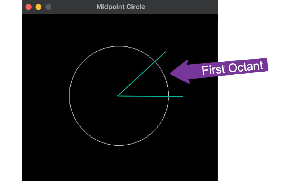
Figure 3.9: The result of the midpoint circle algorithm with the first octant highlighted
While the Pygame API makes drawing lines and circles straightforward, now having examined Bresenham’s algorithms at a pixel-by-pixel level, you’ll have a deeper understanding of the mathematics that is going on behind the scenes.
However, the lines and circles we have produced in this section look rather jagged close up. The reason for this will now be revealed and solutions posed to create smoother lines.
Anti-aliasing
In the previous sections, we worked on producing pixel-by-pixel lines where one pixel was chosen over another in order to create a continual line or circle. If you zoom in on these pixels, however, you will find that they are quite jagged in appearance, as illustrated by the zoomed-in section of a circle shown in Figure 3.10:

Figure 3.10: A zoomed-in section of the Bresenham circle pixels
This effect occurs because of the way that integer values are chosen to represent the drawing. However, when we looked at the actual equations for lines and circles in the The Naïve Way: Drawing a line with brute force and Drawing Circles the Bresenham way sections, it was clear they involved floating-point values and seemed to pass through more than one pixel. To improve the look of these kinds of drawings, a process called anti-aliasing is employed to blur the pixels that are neighbors of the line pixels to fade the edges of the line. Figure 3.11 shows the zoomed-in edge of a black shape that is aliased (Figure 3.11(a)) and anti-aliased (Figure 3.11(b)):

Figure 3.11: A zoomed-in section of a shape without (a) and with (b) anti-aliasing
There are several techniques for achieving anti-aliasing that make rasterized digital images appear a lot smoother, including multisampling, supersampling, and fast approximation. For further details on these algorithms, refer to en.wikipedia.org/wiki/Anti-aliasing.
In short, however, these algorithms work by considering the color of their neighboring pixels and averaging out the colors between them to create a blur or tweening effect between the two. In the case of drawing black pixels on a white background, wherever the contrast difference between the two is greatest, gray pixels are used to smooth out the jagged edge.
In the case of geometry, instead of considering whether a pixel is part of the shape or not, that is, considering it true if it is a part of the line and false if it isn’t part of the line, it’s given a weight based on how much of the line covers it. This is shown in Figure 3.12 with a close-up of a line segment that is 1 pixel wide, as defined by the rectangle in Figure 3.12(a). In Figure 3.12(b), the pixels mostly covered by the line are black and then, depending on how much of the line covers the other pixels, they are weighted with lesser values of gray:

Figure 3.12: Anti-aliasing according to weighting pixels
In most engines, anti-aliasing is an option that can be turned on and off. It’s usually applied as a postproduction effect, and therefore requires the image to be processed twice: once for drawing and a second time for anti-aliasing. If you are interested in drawing and comparing an anti-aliased circle with Pygame, you can try out the following code:
from pygame import gfxdraw
# Without anti-aliasing
pygame.draw.circle(screen, white, (500, 500), 200, 1)
# With anti-aliasing
pygame.gfxdraw.aacircle(screen, 500, 500, 210, white)
Anti-aliasing will make a big difference to the visual quality of your graphics applications, so be sure to look out for it as a setting in any software you are using.
Summary
In this chapter, we’ve created code to force the errors incurred when trying to plot floating points in whole-number pixel locations. Mathematically speaking, the focus of the chapter was on Bresenham’s algorithms for drawing lines and circles that take the respective equations and create a raster image from them while working with integer values to ensure a pixel-perfect drawing.
In Chapter 4, Graphics and Game Engine Components, we will explore the structure of graphics engines and look at how they are put together to cater to the numerous functions they need to serve.