5

Let’s Light It Up!

While we will take a closer look at rendering techniques in depth later on in the book, it always brings a sense of achievement when you can get some color on the screen. Not just a sprite and a pretty background, but painting 3D objects with light and texture.

In this chapter, I will go over the fundamental ways that OpenGL works with light and textures to give you more to experiment with as you continue to investigate these types of projects. You will learn how to add lighting and materials to the project we are developing throughout. It will provide you with the skills to develop better-rendered images that will assist you in visual confirmation that your code is working as it should.

In this chapter, we will cover the fundamentals of visualization, including the following:

• Adding Lighting Effects
• Placing Textures on Meshes

Technical requirements

In this chapter, we will be using Python, PyCharm, and Pygame, as used in previous chapters.

Before you begin coding, create a new folder in the PyCharm project for the contents of this chapter called Chapter_5.

The solution files containing the code can be found on GitHub at https://github.com/PacktPublishing/Mathematics-for-Game-Programming-and-Computer-Graphics/tree/main/Chapter05.

Adding Lighting Effects

Lighting in computer graphics serves the same purpose as it does in the real world. It provides definition to the rendering of objects, making them seem embedded in the virtual world. The way that light is perceived depends on the surface treatment of the objects. These treatments are defined as materials and will be discussed in the next section.

Light sources consist of three primary lighting interactions:

• Ambient light represents the background light in an environment that doesn’t emanate from anywhere. It’s like the light that you can still see in a room when all the lights are out, but you can still make out the shapes of objects because light might be leaking into the room through windows. It is light that has been reflected and scattered so much that you can’t tell where it is coming from. It’s a basic coloring and although it doesn’t emanate from a particular source, in computer graphics, it is assigned as part of a light source.
• Diffuse light comes from the light source and illuminates the geometry of an object, giving it depth and volume. The surfaces of the object that face the light are the brightest.
• Specular light bounces off a surface and can be used to create shiny patches. As with diffuse light, specular light comes from the direction of the light source, and the surfaces of the object that face the light are the brightest.

Each of these can have a color assigned to produce differing effects. The results of each can be seen in Figure 5.1:

Figure 5.1: The components of light that make up a final render

With the exception of ambient light, which is applied uniformly over a model, the way light is seen on an object is by the way that it is reflected. There are numerous models, called shading models, that define the mathematics involved in generating this light on surfaces in graphics. The two types are called diffuse scattering and specular reflection. While these will be elucidated in later chapters, it is worth an overview of how they work before we try them in Python with OpenGL. Figure 5.2(a) illustrates the important directions involved when calculating light intensities. The light source shines at a point on a surface. The light from this point is reflected to the viewer. In the simplest illumination model, the light will be seen at its most intense when viewed at the same reflected angle around the surface normal (indicated by n).

Diffuse scattering (see Figure 5.2(b)) occurs when incoming light is partially absorbed by a surface and is re-radiated uniformly in all directions. Such light interacts with the surface material of the object and as such, the light’s color is affected by the surface color. It makes no difference which angle the surface is viewed from. In Figure 5.2(b), a viewer at v1 and a viewer at v2 will experience the same intensity of light coming from the surface:

Figure 5.2: The components of light that make up a final render

Specular reflections are highly directional. Unlike diffuse scattering, it does matter where the view is in relation to the light source. The intensity of the light will be strongest where the incoming light angle and reflected light angle are the greatest but then drop off away for angles greater or less than. For example, in Figure 5.2(c), a viewer at v1 will see a stronger light intensity than the viewer at v2.

It’s probably time to look at turning on the lights in a Python application.

Let’s do it…

In this exercise, we will explore how lights are enabled and used in OpenGL. Be sure to create a new folder called Chapter_Five in which to place the files for these exercises, and then follow these steps:

1. Create a new Python script called HelloLights.py and copy the exact same code from the previous rotating cube in the Chapter 4, Graphics and Game Engine Components script in HelloMesh.py.
2. Edit Mesh3D.py and change the line from this:

   glBegin(GL_LINE_LOOP)

Change it to this:

glBegin(GL_POLYGON)

3. Run this application. You will get a black window with the white silhouette of a solid rotating cube.
4. Now, modify HelloLights.py with the following lines:

   done = False

   white = pygame.Color(255, 255, 255)

   glMatrixMode(GL_PROJECTION)

   gluPerspective(60, (screen_width / screen_height),

                  0.1, 100.0)

   glMatrixMode(GL_MODELVIEW)

   glTranslatef(0.0, 0.0, -3)

   glEnable(GL_DEPTH_TEST)

   mesh = Cube()

The code has become a little more complex and introduces a few new OpenGL calls, including the following:

• glMatrixMode(): As we have not yet covered matrices in this book, for now, just think of them as changing coordinate spaces. There are two calls for glMatrixMode(). First, we go into the projection view to set up the camera and its coordinate system. Next, we change to the modelview that allows us to specify coordinates in the world space. Working in world space coordinates is far more intuitive.
• glEnable(GL_DEPTH_TEST): Ensures that fragments (pixels yet to be drawn) behind other fragments with respect to the camera view are discarded and not processed, making rendering more efficient.

5. Let’s turn on some lights. Add in the code to enable them:

   ..

   glTranslatef(0, 0, -4)

   glEnable(GL_DEPTH_TEST)

   glEnable(GL_LIGHTING)

   while not done:

   ..

Now, when you run the application, the lights will be on, but they might not look like they are because you will see a very dull version of the rotating cube. This is a kind of ambient lighting. Just because the lights are enabled doesn’t spontaneously create any lights. We have to do that manually.

6. To create a light and turn it on, add the following:

   ..

   glEnable(GL_DEPTH_TEST)

   glEnable(GL_LIGHTING)

   glLight(GL_LIGHT0, GL_POSITION, (5, 5, 5, 1))

   glEnable(GL_LIGHT0)

   while not done:

   ..

Let’s look at what we’ve done here:

• glLight() defines the first light called GL_LIGHT0 as indicated by the first parameter. This is an internal symbol used by OpenGL and as such, you can have GL_LIGHT1, GL_LIGHT2, and so on, up to GL_MAX_LIGHTS (which is an OpenGL internal value you can print out to determine how many lights you have access to with your graphics card).
• The second parameter of glLight() indicates what you want to do with the light. In this case, you are setting the position and placing it at (5, 5, 5) in world coordinates. You will note here that instead of a three-coordinate value for the light position, it is given as four values. The fourth value is w and is important in matrix calculations. For now, just leave it as 1.
• glEnable(GL_LIGHT0) turns on the light.

7. To control the ambient, diffuse, and specular colors from GL_LIGHT0, add the following:

   ..

   glLight(GL_LIGHT0, GL_POSITION, (5, 5, 5, 1))

   glLightfv(GL_LIGHT0, GL_AMBIENT, (1, 0, 1, 1))

   glLightfv(GL_LIGHT0, GL_DIFFUSE, (1, 1, 0, 1))

   glLightfv(GL_LIGHT0, GL_SPECULAR, (0, 1, 0, 1))

   glEnable(GL_LIGHT0)

   ..
8. Run the application to see a fully lit cube, as shown in Figure 5.3:

Figure 5.3: A cube with lighting enabled

Each of the given light types is succeeded by a four-valued red, green, blue, and alpha (transparency) value. The light will be positioned in the world at (5, 5, 5) and have a magenta ambient color, a yellow diffuse color, and a green specular color. Note that OpenGL requires color channel values to be specified between 0 and 1.

You can run this application to see the effect as well as play around with turning the light types off and changing the color. Be aware that at this stage, you might find it difficult to get any specular lighting to appear with these very few settings. It’s sometimes easier to see if you revolve the model around, as there will be a glint in the corners.

Your turn…

Exercise A: Change the ambient color of GL_LIGHT0 to green.

Exercise B: Add a new light symbolized by GL_LIGHT1 and place it at (-5, 5, 0). Set its diffuse light to blue and don’t forget to enable the light.

There’s so much more to lighting systems in graphics than has been covered here. Although they are very complex, at this stage in the book, it’s just exciting to see some lights on the models we are rendering.

In addition to lights, the surface treatment of objects is also important to their appearance. We’ll add some materials in the next section.

Placing Textures on Meshes

Materials are the surface treatments given to polygons that make them appear solid. The coloring-in of the polygon plane gives the illusion that it has substance and is more than its surrounding edges. The surface treatment applied interacts with the lighting applied to give the final appearance.

Just like lights, materials have different ambient, diffuse, and specular colors. Each of these interacts with the corresponding lights to determine the final effect seen. For example, white diffuse light shone on a diffuse green cube will reflect the color green. Although white light is hitting the cube, the green color of the cube determines what light gets reflected. White light is when all the color channels for R, G, and B are turned on, hence the (1, 1, 1) value. If the cube is green, then its color is set to (0, 1, 0). Essentially, it’s the channel that the light and the material both have turned on that is reflected. Of course, it is a little more complex than that, as color channels can take on any value between 0 and 1, but you get the idea.

The process of adding materials is possibly even more complicated than lighting and there’s no better way of learning how to code with them than jumping right in.

Let’s do it…

The best way to see and understand this effect is to experiment with it, so let’s get started by following these steps:

1. From your previous HelloLights.py code, remove any extra lights that you might have created and for the single light left, set only the diffuse color to (1, 1, 1) and add these extra lines, which will add a material onto the cube:

   glEnable(GL_LIGHTING)

   glLight(GL_LIGHT0, GL_POSITION, (5, 5, 5, 1))

   glLightfv(GL_LIGHT0, GL_DIFFUSE, (1, 1, 1, 1))

   glEnable(GL_LIGHT0)

   glMaterialfv(GL_FRONT, GL_DIFFUSE, (0, 1, 0, 1));

   while not done:

Run this to see the green cube. White light falling onto a green object will display that object as green.

2. Now change the light’s color from white to yellow, for example, (1, 1, 0, 1). Run this. The cube is still green. Why? Well, the cube is green, and the light has both red and green channels. The red channel is absorbed by the teapot while the green channel is reflected. So, the effect is the same as before.
3. Now change the light’s color from yellow to red, for example, (1, 0, 0, 1). Run this. You get a very dark colored almost black, except for that background ambient light cube. Why? Because the red light shining on the cube is fully absorbed and there’s nothing left to reflect.

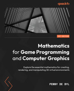
Besides coloring the surface of an object with lights and pure color, an external image can be used. This image is called a texture as it can be used to add a haptic quality to the object’s surface. Textures are placed on the surface of an object, polygon by polygon, through a process called texture mapping. This mapping occurs by giving each corner of the texture a two-dimensional coordinate with values ranging between 0 and 1. The horizontal values of the texture are akin to the x axis; however, in this process, they are referred to as u. The vertical values, like the y axis, are referred to as v. Hence the coordinates of a texture are called UVs. The UV values are matched to specific vertices as shown in Figure 5.4; the UVs that match the bottom-right triangle of a square are highlighted:

Figure 5.4: Texture Mapping

Working with External Files

From this point onwards in the book, we will be working with files that are external to the Python script. Throughout the book, the code assumes the external files (models, textures and shaders) are in the same folder as the code accessing them. However, in GitHub repository of this book, the external files are accessed as if one folder higher. Please keep this in mind for referencing external files in the code.

For example, if your project files are organized like this:

Root folder

- Project 1

--- Main.py

--- Models

------ Teapot.obj

It means that the models folder containing the teapot model is in the same folder as the main.py code. To reference Teapot.obj from inside Main.py the address is:

Models/Teapot.obj

However, if you would like to keep the external files in one place and outside of any particular chapter project, you can place them on the same level as each chapter code (as is referenced in GitHub repository of this book). This structure appears as:

Root folder

--- Project 1

------ Main.py

--- Models

------ Teapot.obj

In this case, the address of Teapot.obj should be:

../Models/Teapot.obj

The ../ in the file address tells the code to look up one folder from where the code is running from.

The best way to get to understand UVs is to start using them. The way that OpenGL binds the texture to vertices might seem a little long-winded, but you will soon understand the process in order to apply it elsewhere.

Let’s do it…

Work through these steps to place textures onto the models by controlling the UVs:

1. Before adding in a texture and performing some UV mapping with our cube, we will make a few modifications to the existing Mesh3D and Cube classes. First, in the Mesh3D class, add the following:

   class Mesh3D:

     def __init__(self):

       …

       self.triangles = [0, 2, 3, 0, 3, 1]

       self.draw_type = GL_LINE_LOOP

       self.texture = pygame.image.load()

       self.texID = 0

These three lines create extra variables we can use to set how a mesh will be drawn and what, if any, texture to use.

Next, we modify the Cube class to set the values of these new variables:

class Cube(Mesh3D):
  def __init__(self, draw_type, filename):
    self.vertices = …
    self.triangles = …
    Mesh3D.texture = pygame.image.load(filename)
    Mesh3D.draw_type = draw_type

Note that we will be passing through draw_type and a filename from main script. However, before we do that, we should add a texture file.

2. Visit textures.com and find a texture that you would like to map onto the cube. Select one that is 512 x 512. Download the texture and add it to PyCharm in the same manner used in Chapter 1, Hello Graphics Window: You’re On Your Way. Take note of the path to this image for use in your code.
3. Edit the mesh creation line in HelloLights.py to accept the new parameters:

   mesh = Cube(GL_POLYGON, "images/brick.tif")

Note that where I have the path to my image, you should replace it with yours.

4. At this point, you might like to run the code to check you haven’t introduced any syntax issues. There will be no difference in the cube. It will draw as a solid and use the lighting settings from the previous exercise.
5. Now, add the new method to the Mesh3D class:

   def init_texture(self):

     self.texID = glGenTextures(1)

     textureData = pygame.image.tostring(self.texture,

                                         "RGB", 1)

     width = self.texture.get_width()

     height = self.texture.get_height()

     glBindTexture(GL_TEXTURE_2D, self.texID)

     glTexParameteri(GL_TEXTURE_2D,

                     GL_TEXTURE_MIN_FILTER,

                     GL_LINEAR)

     glTexImage2D(GL_TEXTURE_2D, 0, 3, width, height, 0,

                  GL_RGB, GL_UNSIGNED_BYTE, textureData)

This method takes the image loaded with Pygame and loads it into OpenGL by doing the following:

• Using glGenTextures() to create a unique ID for the texture that can be used by OpenGL.
• Calling glBindTexture(), which sets the new ID to the type of texture being created, which in this case is a normal 2D image.
• Running glTexParameteri() sets up the function used by the texture for a variety of methods. In this case for working with this GL_TEXTURE_2D, the function of GL_TEXTURE_MIN_FILTER (which determines how lower resolutions of a texture are used to blur an image with distance from the camera) is set to GL_LINEAR, which provides a linear distance falloff for this blurring effect. This is also referred to as mipmapping and will be covered in depth in later chapters.
• Generating the OpenGL texture from the given image file and binding it to the texture ID given in the preceding glBindTexture() call.

6. The preceding method can now be called at the very bottom of the __init__() method in the Cube class:

   Mesh3D.texture = pygame.image.load(filename)

   Mesh3D.draw_type = draw_type

   Mesh3D.init_texture(self)
7. With all this setup done, it’s time to define the UV values. There needs to be one UV for each vertex that has been given where the UVs are in the same order as the vertex to which they are mapped. In the Cube class, add this new set of UVs like this:

   self.triangles = …

   self.uvs = [(0.0, 0.0),

         (1.0, 0.0),

         (0.0, 1.0),

         (1.0, 1.0),

         (0.0, 1.0),

         (1.0, 1.0),

         (0.0, 1.0),

         (1.0, 1.0),

         (0.0, 0.0),

         (1.0, 0.0),

         (0.0, 0.0),

         (1.0, 0.0),

         (0.0, 0.0),

         (0.0, 1.0),

         (1.0, 1.0),

         (1.0, 0.0),

         (0.0, 0.0),

         (0.0, 1.0),

         (1.0, 1.0),

         (1.0, 0.0),

         (0.0, 0.0),

         (0.0, 1.0),

         (1.0, 1.0),

         (1.0, 0.0)]

   Mesh3D.texture = pygame.image.load(filename)
8. With the UV values in place, the draw() method in the Mesh3D class can be updated:

   def draw(self):

     glEnable(GL_TEXTURE_2D)

     glTexEnvf(GL_TEXTURE_ENV, GL_TEXTURE_ENV_MODE,

               GL_DECAL)

     glBindTexture(GL_TEXTURE_2D, self.texID)

     for t in range(0, len(self.triangles), 3):

       glBegin(self.draw_type)

       glTexCoord2fv(self.uvs[self.triangles[t]])

       glVertex3fv(self.vertices[self.triangles[t]])

       glTexCoord2fv(self.uvs[self.triangles[t + 1]])

       glVertex3fv(self.vertices[self.triangles[t + 1]])

       glTexCoord2fv(self.uvs[self.triangles[t + 2]])

       glVertex3fv(self.vertices[self.triangles[t + 2]])

       glEnd()

OpenGL draws through the enabling and disabling of facilities with differing method calls. These switch OpenGL into different processing states. In this case, at the beginning of the draw() method, texture mapping is enabled with glEnable(GL_TEXTURE_2D). The glTexEnvf()function sets up the texture environment that determines how texture values are interpreted for the purpose of generating an RGBA color value. Put simply, the GL_DECAL parameter keeps the incoming texture pixel RGBA values the same as they are in the source image. The particulars of this method are quite complex and for more information, you are encouraged to look at the following: https://www.khronos.org/registry/OpenGL-Refpages/gl2.1/xhtml/glTexEnv.xml.

Next, you will notice the use of glBindTexture() again. This tells OpenGL which texture we want to work with.

Following this, the code enters the for loop previously used to draw the wireframe and solid cubes. Notice the code remains relatively the same with the exception that the UV values are set before the vertices they match with. As we have a UV value for each vertex and each triangle keeps track of the vertices used, the code can also refer to the correct UV values.

9. Run the code. You will see a rotating solid cube with the texture given mapped across the surface, as shown in Figure 5.5:

Figure 5.5: A texture mapped onto a cube

This exercise has covered UV values and their use for mapping a texture onto a 3D object. As you can see, the process involves a lot of arrays of values. These arrays include the vertex list and another list for UVs where each vertex is assigned a UV in order to get the texture perfectly aligned with the geometry.

Summary

This chapter has been a short examination of lighting and texture that help to bring depth to a scene and make objects appear solid. Besides the lists of vertices and UVs that we’ve used, you will discover later in the book that a 3D mesh can possess many other sets of values used for a multitude of rendering effects. But for now, you have enough skill in displaying a simple mesh and adding a texture to it.

In the next chapter, we will add more flexibility to the project we are creating by working more with the main loop. In addition, we will improve the application architecture to make it more extensible by giving simple rendered objects access to more behaviors.

Answers

Exercise A:

glLightfv(GL_LIGHT0, GL_AMBIENT, (0, 1, 0, 1))

Exercise B:

glLightfv(GL_LIGHT0, GL_SPECULAR, (0, 1, 0, 1))
glEnable(GL_LIGHT0)
glLight(GL_LIGHT1, GL_POSITION, (-5, 5, 0, 1))
glLightfv(GL_LIGHT1, GL_DIFFUSE, (0, 0, 1, 1))
glEnable(GL_LIGHT1)
while not done: