16
Rotating with Quaternions
If you can’t remember me saying it before, you’ll be sure to hear me say it numerous times throughout this chapter: quaternions are an advanced mathematical construct. They are so advanced I don’t expect you to fully comprehend them by the end of this chapter. However, what I want you to take away is a healthy appreciation for what they do with respect to solving the gimbal lock issue we discussed in Chapter 15, Navigating the View Space.
Besides their usefulness in calculating 3D rotations, quaternions are useful in numerous fields, including computer vision, crystallographic texture analysis, and quantum mechanics. Conceptually, quaternions live in a 4D space through the addition of another dimension to those of the x, y, and z axes used by Euler angles.
In this chapter, we will start with an overview of quaternions and delve into the benefits of their 4D structure. This will reveal how they can be used to replace operations for which we’ve previously been using Euler rotations. We will then jump back into our Python/OpenGL project and update the rotation methods to use quaternions.
In this chapter, we will be doing the following:
- Introducing quaternions
- Rotating around an arbitrary axis
- Exploring quaternion spaces
- Working with unit quaternions
- Understanding the purpose of normalization
By the end of this chapter, you will have developed the skills to use quaternions in place of Euler angles for compound rotations in graphics applications. Furthermore, you’ll have a firm grasp on quaternion concepts and be set up to independently explore the concept in more detail for other applications.
Technical requirements
In this chapter, we will be using Python, PyCharm, and Pygame, as used in previous chapters.
Before you begin coding, create a new folder in the PyCharm project for the contents of this chapter called Chapter_16.
The solution files containing the code can be found on GitHub at https://github.com/PacktPublishing/Mathematics-for-Game-Programming-and-Computer-Graphics/tree/main/Chapter16.
Introducing quaternions
The minimum number of values needed to represent rotations in 3D space is three. The most intuitive and long-applied method for defining rotations, as we’ve seen, is to use these values as the three angles of rotation around the x axis, the y axis, and the z axis. The values of these angles can range from 0 to 360 degrees or 0 to 2 PI radians.
Any object in 3D space can be rotated around these axes that represent either the world axes or the object’s own local access system. Formally, the angles around the world axes are called fixed angles, while the angles around an object’s local axis system are called Euler angles. However, often both sets of angles are referred to as Euler angles. We covered the mathematics to apply rotations around these three axes in Chapter 15, Navigating the View Space, in addition to investigating when these calculations break down and cause gimbal lock.
Quaternions were devised in 1843 by Irish mathematician William Hamilton for applications to mechanics in 3D space. They can be applied in numerous areas of mathematics, and when Hamilton came up with them, he wasn’t even thinking about rotations but rather how to calculate the quotient of two coordinates in 3D space. Put simply, this means being able to perform divisions between coordinates. It’s easy enough to add and subtract 3D points and vectors from each other, but how do you multiply and divide them? Hamilton came up with the idea of using four dimensions rather than three. To help you understand the use of four dimensions in a calculation, let’s go back to the very beginning of rotational mathematics with those in 2D space.
Rotating around an arbitrary axis
A vector lying on the x axis that is represented by (1, 0) and rotated by ![]() results in the vector that will be the cosine of the angle and the sine of the angle (
results in the vector that will be the cosine of the angle and the sine of the angle (![]() as illustrated in Figure 16.1. Likewise, a vector sitting on the y axis represented by (0, 1), when rotated by the same angle, will result in a vector that, too, contains a combination of cosine and sine as (-
as illustrated in Figure 16.1. Likewise, a vector sitting on the y axis represented by (0, 1), when rotated by the same angle, will result in a vector that, too, contains a combination of cosine and sine as (-![]() .
.

Figure 16.1: Two-dimensional rotations
Do these values look familiar? They should because they are the values we’ve used in the rotation matrix for a rotation around the z axis in Chapter 15, Navigating the View Space. Rotating in 2D is essentially the same operation as rotating around the z axis; as you can imagine, the z axis added to Figure 16.1 coming out of the screen toward you, and thus rotations in this 2D space are, in fact, rotating around an unseen z axis.
All the rotations we’ve looked at thus far have been to rotate a vector or point around an x, y, or z axis. As for the case of rotating in the 2D space of the x/y plane, which is a rotation around the z axis, any of these 3D rotations can be reduced to 2D where a rotation around the y axis occurs on the x/z plane, and a rotation around the x axis occurs on the y/z plane. This is illustrated in Figure 16.2:

Figure 16.2: Rotations around the z and x axes represented on a plane
Taking this one step further is the Euler-Rodrigues theorem, which allows for rotations around an arbitrary vector in space, where this vector becomes the rotational axis. This 3D rotation can also be simplified to a 2D rotation, as shown in Figure 16.3. If you consider the 3D rotation of a vector around another vector (u), the tip of the first vector will form a circle in space as it rotates through 360 degrees. This circle represents a plane. Just like the x/y plane in a z rotation. Though the representation of this plane isn’t as simple, as we are in a completely different coordinate system that we can’t just attribute to straightforward x, y, and z world axes. However, it is still a flat surface and if looked at down the rotational axis, it becomes a 2D rotation, as shown on the right in Figure 16.2:

Figure 16.3: Rotations around an arbitrary axis in 3D (left) and reduced to 2D (right)
As previously stated, although we appear to have a nice simple rotation in 2D, because we’ve moved out of the regular x, y, and z axis system and are now in a different frame of reference, the mathematics becomes somewhat complex. For those of you who are interested, the rotational matrix for rotating around the arbitrary vector u is as follows:

In this format, the mathematics is indeed overwhelming, though not beyond your abilities to program it into your project and use it. However, if we reduce this matrix down to its basic components of the rotational axes u, the vector to be rotated v, and the angle of rotation ![]() , the formula becomes:
, the formula becomes:
![]()
Note here how the familiar terms for ![]() and
and ![]() come out again, just like they did for the original 2D rotations. And that’s because although you’ve had to use a lot of mathematics to find the plane of rotation relative to the world x, y, and z, the operation is the same.
come out again, just like they did for the original 2D rotations. And that’s because although you’ve had to use a lot of mathematics to find the plane of rotation relative to the world x, y, and z, the operation is the same.
As a reader of this book, I don’t expect you to fully embrace the mathematics (unless you want to) as it’s university master’s level stuff. However, I would like you to appreciate the beauty of it. The main point I’m focusing on is that if you can represent 3D rotations as 2D rotations, then you must be able to represent 4D rotations as 3D rotations. Wrapping your mind around this concept is key to understanding how quaternions work.
Now, you might be wondering if the Rodrigues-Euler Theorem solves the issue of gimbal lock. The answer is, unfortunately, no. While the way we’ve been creating complex rotations with Euler angles thus far allows for compound rotations, the Rodrigues-Euler Theorem does not. Therefore, while they look fabulous, we can’t use them in graphics – at least not for complex maneuvers. This is because each rotation that occurs is in a different frame of reference.
Therefore, the solution resides in the four-dimensionality of quaternions, as will soon be revealed.
Exploring quaternion spaces
As we saw in Chapter 13, Understanding the Importance of Matrices, 4 x 4 matrices are important in graphics as they allow for easy multiplication of compound transformations. Although I didn’t make a big deal of it at the time, these matrices are, in fact, four-dimensional as they have four columns and four rows. Just as we need 4 x 4 matrices to multiply transformation operations, Hamilton found he could use them to find quotients of 3D values. However, the process is a little more complex than how we just created a w dimension for coordinates with a 1 or a 0 on the end for (x, y, z, w).
So, where did Hamilton find his fourth dimension? He had to add another number system and he turned to complex numbers. If you aren’t familiar with complex numbers, then take a look at the explanation here: https://en.wikipedia.org/wiki/Complex_number.
In short, complex numbers were devised for solving quadratic equations and to come up with a solution to finding the square root of a negative one. The solution was denoted i, thus:
![]()
In this case, i is an imaginary number.
With respect to representing 3D coordinates as 4D coordinates, the imaginary axis is added. Complex numbers contain an imaginary part and a real part. The real part is 3D space, as you already understand it. Complex numbers are written with both parts thus:
![]()
Representing this on a 2D graph looks like the image in Figure 16.4. A point is defined by a horizontal component, which is the real part, and an imaginary component, which is the vertical part. This is not unlike using x and y to define a coordinate in 2D space once you accept the idea that the real component contains the x, y, and z components:

Figure 16.4: Complex numbers
If we rotate a vector of length 1 with values (a,b) in this space, the result is as follows:

This is the same as the 2D rotations we examined at the beginning of this chapter and illustrated in Figure 16.5. And through this representation, we now have the means to represent a rotation around an arbitrary axis as we did with the Rodrigues-Euler Theorem. The representation of a quaternion is, in fact, an angle and axis stored in four-dimensional space that will allow for compounding operations as the frame of reference remains the same. All rotations occur in the plane real/i.

Figure 16.5: Rotating a vector comprising complex numbers
To visualize quaternions is quite difficult as they are in four dimensions, and to show them on a 2D page is even more of a challenge, but bear with me. We live in a 3D world and are familiar with the three-dimensional axes of x, y, and z. With quaternions, we get the addition of a new axis. To see this, imagine that our 3D world is compressed into a flat disk, as shown in Figure 16.6. The x, y, and z axes live in this space, and the fourth dimension surrounds the flat disk as a sphere. A quaternion represents a point on the outside of this sphere where the sphere’s three dimensions are denoted by three imaginary numbers i, j, and k. A point on the sphere is represented by the coordinate (w, x, y, z) where x is a multiple of i, y is a multiple of j and z is a multiple of k. As an equation, this is as follows:
![]()
You can clearly see in this equation how x, y, and z are scalar values to the imaginary dimensions.
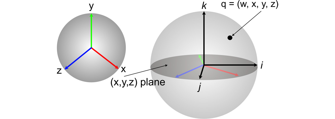
Figure 16.6: Quaternion space
If you aren’t already a little mind-bent, the x, y, and z in quaternion coordinates are not the same values for the x, y, and z of the 3D space and yet this is how mathematicians represent them.
Since quaternions are in 4D space, to use them in graphics programming, we need to convert them into values that make sense in 3D. We know that quaternions represent an angle/axis rotation, but how? If we are rotating a point or vector around an axis, r, by an angle of ![]() then for the quaternion representation
then for the quaternion representation ![]() , the value of w is
, the value of w is  and (x, y, z) =
  where r is a vector in 3D space. Here you can see the cosine and sine playing a role in the rotation. The reason why the angle here is divided by two is to align the quaternion representation to that of Euler-Rodrigues’ Theorem.
To use a quaternion in our project as a rotation, the quaternion converts into a rotation matrix like this:

More on quaternions
The derivation and proof for quaternions go far beyond the scope of this book; however, the interested reader is encouraged to investigate the topic further through these links:
https://www.sciencedirect.com/science/article/pii/S0094114X15000415
http://www.songho.ca/opengl/gl_quaternion.html
https://www.reedbeta.com/blog/why-quaternions-double-cover/
Quaternions, for the novice mathematician, are a very complex and somewhat confusing concept. To really get a feel for them, now that you know the conversion formula, we should start implementing them in our project.
Let’s do it…
In this exercise, we will create a Quaternion class to store the data associated with a quaternion and enable it to perform rotations.
Follow these steps to implement the concept of quaternions in our project:
- Make a copy of the Chapter_15 folder and name it Chapter_16.
- Make a new Python script file and call it Quaternion.py. Add the following code to the newly created file:
from __future__ import annotations
import pygame
import math
import numpy as np
class Quaternion:
def __init__(self, vector=None,
axis: pygame.Vector3 = None,
angle: float = None):
if vector is not None:
self.w = vector[0]
self.x = vector[1]
self.y = vector[2]
self.z = vector[3]
else:
axis = axis.normalize()
sin_angle =
math.sin(math.radians(angle/2.0))
cos_angle =
math.cos(math.radians(angle/2.0))
self.w = cos_angle
self.x = axis.x * sin_angle
self.y = axis.y * sin_angle
self.z = axis.z * sin_angle
Note the very first line of this code, which refers to __future__. For interest’s sake, this allows the Quaternion class to refer to itself inside the body of the class. That is, it is referencing a Quaternion class before the class has been fully described.
The initialization method sets the four values that are used to store a quaternion. The w value is influenced by the cosine operation whereas the x, y, and z values rely on sine. This constructor allows the quaternion properties to be set directly by sending through a vector of four values or by calculating the properties using the axis and angle of rotation.
- Next, we overload the multiplication operation in the class to define how multiplication between quaternions occurs:
def __mul__(self, other: Quaternion):
v1 = pygame.Vector3(self.x, self.y, self.z)
v2 = pygame.Vector3(other.x, other.y, other.z)
cross = v1.cross(v2)
dot = v1.dot(v2)
v3 = cross + (self.w * v2) + (other.w * v1)
result = Quaternion(vector=(self.w *
other.w - dot,
v3.x, v3.y, v3.z))
return result
As you can see, because quaternions are a complex mathematical construct, they can’t be multiplied as easily as numbers in Euclidean space.
- Last but not least, we can use the quaternion to 4 x 4 matrix conversion to return a matrix we can use to multiply with so it can be integrated with our project’s other operations:
def get_matrix(self):
x2 = self.x + self.x
y2 = self.y + self.y
z2 = self.z + self.z
xx2 = self.x * x2
xy2 = self.x * y2
xz2 = self.x * z2
yy2 = self.y * y2
yz2 = self.y * z2
zz2 = self.z * z2
wx2 = self.w * x2
wy2 = self.w * y2
wz2 = self.w * z2
return np.matrix([
[1 - (yy2 + zz2), xy2 + wz2, xz2 - wy2,
0],
[ xy2 - wz2, 1 - (xx2 + zz2), yz2 + wx2,
0],
[xz2 + wy2, yz2 - wx2, 1 - (xx2 + yy2),
0],
[0, 0, 0, 1]
])
- To use the new quaternion-based rotation matrix, we must add a new method into the Transform.py class like this:
from Quaternion import *
..
def rotate_axis(self, axis: pygame.Vector3, angle,
local=True):
q = Quaternion(axis=axis, angle=angle)
r_mat = q.get_matrix()
if local:
self.MVM = self.MVM @ r_mat
else:
self.MVM = r_mat @ self.MVM
- Make a copy of the recent main file called FlyCamera.py and rename it QuaternionTeapot.py.
- Edit QuaternionTeapot.py to use a quaternion as a rotation in place of our method that used Euler angles like this:
teapot = Object("Teapot")teapot.add_component(Transform())
teapot.add_component(LoadMesh(GL_LINE_LOOP,
"models/teapotSM.obj"))
trans: Transform = teapot.get_component(Transform)
trans.rotate_axis(pygame.Vector3(0, 1, 0), 90)
trans.update_position(pygame.Vector3(0, -2, -3))
- You can now run QuaternionTeapot.py and see the teapot rotated 90 degrees around the y axis. The result will be the same as the previous code, as illustrated in Figure 16.7, in which I used the S key to move the camera away from the teapot to fit it in the window:

Figure 16.7: Rotating the teapot with a quaternion
In this exercise, we have validated rotating an object with a single quaternion by recreating the y axis rotation we achieved in Chapter 15, Navigating the View Space. When introducing a new mathematical method, to ensure it behaves as you believe it should, always find another way to achieve the same result if possible.
This section has been a whirlwind look at quaternions. As you will appreciate, they are a highly complex mathematical construct. Even if you don’t fully understand all the mathematics involved, it has been my intention that you will at least appreciate what they can do and how they can be implemented in code. However, we didn’t just add quaternions in to make single rotations more complex; their power in graphics is to remove any issues related to the gimbal lock inherent with Euler angles. We will now discuss this topic and modify our project appropriately.
Working with unit quaternions
As discussed, quaternions remove the limitations involved in compounding Euler-angle rotations. In this section, we will concentrate on reprogramming the camera in our project to pitch and roll with quaternions.
Before quaternions are multiplied, we must ensure they are unit quaternions. That means they will have a length of 1. If we go back to thinking of quaternion spacing being a sphere encompassing Euclidean space, then a quaternion represents a vector from the origin of both spaces to the surface of the sphere. In Figure 16.9, the vectors q1 and q2 represent these. The vector representing a quaternion is four-dimensional, with the coordinates storing the angle and axis as  .
.
Of course, you must remember we can’t see these four dimensions in our 2D/3D sphere diagram, but they are there. In Figure 16.8, q3 represents an invalid quaternion in that it extends beyond the surface of the sphere. However, the rotation that it is meant to represent can be found by normalizing its vector representation back to a length of 1, shown by vector q4. This unit length vector now points nicely to the surface of the sphere, or quaternion space, instead of beyond it:

Figure 16.8: Unit quaternions
The next question you should be asking is, “how do I normalize a quaternion?” It’s a matter of finding the length of the quaternion and dividing each component by that length in the same way we normalized vectors in Chapter 9, Practicing Vector Essentials. To find the length of a quaternion, we can use Pythagoras’ Theorem, where the length of a quaternion is calculated with the following:
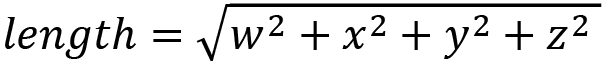
The normal form of the quaternion is then:

Let’s see if you can now use this knowledge to create a method to produce a normal vector.
Your turn…
Exercise A:
Using your understanding of normalizing vectors, write down on a piece of paper pseudocode to produce a normalized quaternion.
In this section, we have discussed the importance of unit quaternions. But why aren’t they always in unit form? Let’s take a look.
Understanding the purpose of normalization
If you are wondering why we need to normalize a quaternion in the first place, it’s because the values used to create it may produce a quaternion with a length longer than 1, especially if it’s code that you are adding yourself.
Take, for example, the 3D process of moving an object along a vector at a constant speed. In Chapter 10, Getting Acquainted with Lines, Rays, and Normals, we moved an object along a line segment at a constant speed. To achieve a constant speed, we needed to take into consideration the time between frames so we could factor in any changes. The code we created moved an object in equal steps from one end of a line segment to the other. Taking this same idea, we can write code to move an object in 3D along a vector at a constant speed. The essential parts of this script would look something like this:
dt = 0
direction = (0, 0, 0.1)
while not done:
  new_position = old_position + (direction * dt)
  dt = clock.tick(fps)
In this case, the object doesn’t have an ending location; it just moves along the direction vector multiplied by the time between frames each frame. Now, if direction becomes a calculated value, say we want to move the object between its current location toward another object, the length of direction will become crucial. Consider the tanks in Figure 16.9. They are to move toward the palm tree. The direction of the red tank to the tree is calculated with the following:
v = tree_position – red_tank_positionThis situation is visualized in Figure 16.9:

Figure 16.9: Two objects moving toward a destination
Likewise, the vector u is calculated to be as follows:
u = tree_position – green_tank_positionThe distance the red tank is from the tree will be the length of the vector v, and the distance the green tank is from the tree will be the length of the vector u. For the sake of this example, let’s say that the length of v is 10, and the length of u is 7.
If we move each tank along its associated vector in one frame, the red tank will move 10 units per frame and the green tank, 7 units per frame. We can agree that makes the red tank faster as it covers more distance in the same amount of time. If, however, we want both these tanks to move at the same speed, we can find the unit vectors in the direction of travel. As both unit vectors, no matter which way they are facing, have a length of 1, when we add 1 to both tanks in each frame, they will be traveling at the same speed. Even if we multiply their unit direction vectors by the time between frames, they will still move at the same rate. A partial listing of the logic of this code looks like this:
dt = 0
red_direction = tree_position – red_tank_position
green_direction = tree_position – green_tank_position
red_normalised = red_direction/red_direction.magnitude
green_normalised =
    green_direction/green_direction.magnitude
while not done:
 red_tank_position = red_tank_position + (red_normalised *
                                          dt)
 green_tank_position = green_tank_position +
                       (green_normalised * dt)
 dt = clock.tick(fps)
This example shows where unit vectors are useful and how they are calculated in code. The same issue can also occur when human input is required. Let’s say you want the tanks to move in a 45-degree direction on the x/z plane, as shown in Figure 16.10.
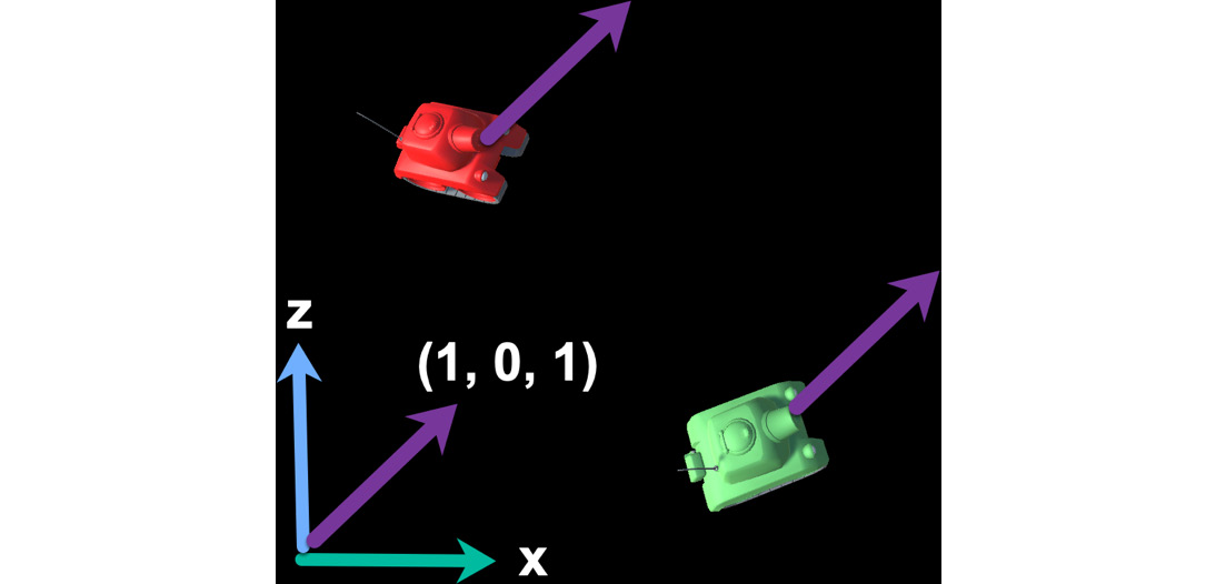
Figure 16.10: Specifying a movement direction
A 45-degree vector on the x/z plane can be denoted (1, 0, 1). This makes sense as it has equal parts of x as it does of z, hence cutting the 90-degree angle between the x axis and the z axis in half. Similarly, the vector (0.5, 0, 0.5) and (3, 0, 3) are also 45-degree vectors pointing in the same direction. Though, which of all these is a unit vector? The answer is none of them. If you normalize each of these vectors, you will find the unit vector in the same direction:

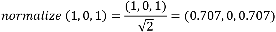


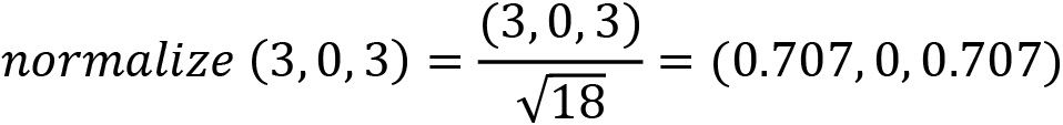
Notice how all the calculations result in the same vector? That’s because all the original vectors pointed in the same direction.
So, whether you find it easier to manually set a vector using your intuition, such as using (1, 0, 1) instead of (0.707, 0, 0.707), or a distance calculation happens in the code, and then a unit vector needs to be found, being able to normalize a vector is a useful operation.
The same goes for quaternions. Possibly even more so, as it’s going to be more intuitive to say you want to rotate an object around the axis (1, 0, 1) with an angle of 45 than being concerned if the resulting quaternion has a length of 1. Therefore, being able to normalize vectors and quaternions is key for consistency in mathematics.
This brings us back to the matter of being able to normalize a quaternion, which we achieved in the previous section. Now it’s time to implement the normalization in our project and use it for compounding rotations.
Let’s do it...
In this exercise, we will write up the code for normalizing a quaternion and then use it to ensure all quaternions that are multiplied together are a length of 1. Having achieved this, we will begin testing the multiplication overload in the Quaternion class:
- To the Quaternion class in Quaternion.py, add a normalize method and use it when a quaternion is constructed, as follows:
import sys
..
class Quaternion:
def __init__(self, vector=None, axis: pygame.Vector3 =
None, angle: float = None):
if vector is not None:
..
else:
axis = axis.normalize()
..
self.z = axis.z * sin_angle
self.normalise()
..
def normalise(self):
length = math.sqrt(self.w * self.w +
self.x * self.x +
self.y * self.y +
self.z * self.z)
if length > sys.float_info.epsilon:
self.w /= length
self.x /= length
self.y /= length
self.z /= length
In this method, the length of the quaternion is found using Pythagoras’ Theorem. This length is then compared to sys.float_info.epsilon. This system variable holds a very small floating-point number that is close to 0. Sometimes when working with floats, a value that would equate to 0 on paper might be stored in the computer fractionally larger than 0. As the length of an essentially 0-length quaternion might be calculated as something close to zero before we divide by the length to get the normalized quaternion, we test that the quaternion has a decent length using epsilon instead of 0.
- To compare the results from using quaternions to those of Euler angles, we will now add two teapots into QuaternionTeapot.py and rotate one with Euler angles and one with quaternions and then compare the results.
- Before you do this, you’ll need to add a new method to the Transform class in Transform.py, as follows:
def rotate_quaternion(self, quaternion: Quaternion,
local=True):
r_mat = quaternion.get_matrix()
if local:
self.MVM = self.MVM @ r_mat
else:
self.MVM = r_mat @ self.MVM
- Modify QuaternionTeapot.py, as follows:
..
objects_3D = []
objects_2D = []
#onleft
euler_teapot = Object("Teapot")euler_teapot.add_component(Transform())
euler_teapot.add_component(LoadMesh(GL_LINE_LOOP,
"models/teapotSM.obj"))
euler_trans: Transform =
euler_teapot.get_component(Transform)
euler_trans.rotate_x(45)
euler_trans.rotate_y(20)
euler_trans.update_position(pygame.Vector3(-3, 0,
-10))
print("Euler Rot")print(euler_trans.get_rotation())
#onright
quat_teapot = Object("Teapot")quat_teapot.add_component(Transform())
quat_teapot.add_component(LoadMesh(GL_LINE_LOOP,
"models/teapotSM.obj"))
quat_trans: Transform =
quat_teapot.get_component(Transform)
q = Quaternion(axis=pygame.Vector3(1, 0, 0), angle=45)
p = Quaternion(axis=pygame.Vector3(0, 1, 0), angle=20)
t = p * q
quat_trans.rotate_quaternion(t)
quat_trans.update_position(pygame.Vector3(3, 0, -10))
print("Quat Rot")print(quat_trans.get_rotation())
camera = Camera(60, (screen_width / screen_height),
0.1, 1000.0)
camera2D = Camera2D(gui_dimensions[0],
gui_dimensions[1], gui_dimensions[3],
gui_dimensions[2])
objects_3D.append(euler_teapot)
objects_3D.append(quat_teapot)
clock = pygame.time.Clock()
..
This new code adds two teapots: one called euler_teapot and one called quat_teapot. Now, euler_teapot is positioned on the left of the screen, and quat_teapot is on the right. Both teapots are first rotated by 45 degrees around the x axis and then 20 degrees about the y axis.
Note that the multiplication for the quaternions occurs in reverse order, such as we used to multiply the transformation matrices in the line t = p * q.
After the rotations have been applied to each teapot, the rotation matrices are printed out for you to compare the results, as sometimes visual cues don’t necessarily give us enough accuracy.
- Run the script to see the two teapots, as illustrated in Figure 16.11. Have they been rotated in the same manner? It is difficult to tell from a perspective view; however, they are facing in similar directions. That’s a good start. However, if you really want to know if the quaternion equations match those of the Euler calculations and vice versa, the only true way to check is to print out the rotation matrices for each, which will be displayed in the console.

Figure 16.11: Rotating teapots with Euler angles and quaternions
In this case, my console is displaying the following:
Euler Rot
[[ 0.93969262  0.         -0.34202014  0.        ]
 [ 0.24184476  0.70710678  0.66446302  0.        ]
 [ 0.24184476 -0.70710678  0.66446302  0.        ]
 [ 0.          0.          0.          1.        ]]
Quat Rot
[[ 9.39692621e-01  1.38777878e-17 -3.42020143e-01  0.0000e+00]
 [ 2.41844763e-01  7.07106781e-01  6.64463024e-01  0.0000e+00]
 [ 2.41844763e-01 -7.07106781e-01  6.64463024e-01  0.0000e+00]
 [ 0.00000000e+00  0.00000000e+00  0.00000e+00  1.0000e+00]]
Yours might display differently if you are on Windows, and you might even have slightly different values to mine. While at first glance, the values look different, they are almost the same. For example, my quaternion matrix has 1.38777878e-17, whereas the Euler matrix has 0. I’m not at all concerned as 1.3 x 10⁻¹⁷ is practically zero, and because we are working with floating-point numbers and performing differing calculations, there are bound to be slight errors. However, these are small enough for us to conclude the quaternion calculations are working as intended.
In this exercise, we have integrated compound quaternion rotations into our project and confirmed they are working correctly by comparing the rotation matrix calculated with an Euler angle calculated based on the same axes and rotations. Now it’s time for you to test your understanding by replacing the Euler movements for the camera with quaternions.
Your turn...
Exercise B:
Reprogram the rotate_with_mouse() method of the Camera class to use a compound quaternion rotation that multiplies the x rotation with the y rotation and then applies it to the camera. The axis of rotation for the x will be the right axis, and for the y, it will be the camera’s up axis. These can be found in the view matrix, as follows:
right = pygame.Vector3(1,0,0)
up = pygame.Vector3(0,1,0)
Summary
In case you missed it the first time, let me say it again: quaternions are an advanced mathematical construct. Though I am sure, by now, you appreciate this statement. They are also extremely powerful, and this chapter has but scratched the surface of all the applications for which they can be applied. Hamilton wasn’t even thinking of 3D graphics rotations when he defined them, but thankfully for us, they exist and remove the inherent issue of compounding Euler angle rotations.
If you’ve reached the end of this chapter and still don’t feel comfortable employing quaternion mathematics, you won’t be alone. In fact, I hesitated to include this chapter as a full comprehension of quaternions requires background knowledge in complex numbers, pure mathematics, and division algebra that we don’t have the scope in this book to include. And if you don’t feel comfortable yet working them, then the simple solution is, don’t. Euler angles will achieve most things you want to do when it comes to rotation. Having said this, as you continue your learning journey in graphics and games programming, you won’t be able to avoid them.
This chapter concludes our exploration of transformations. In the next chapter, we will begin investigating the process of rendering and production of visual effects for graphics.
Answers
Exercise A:
normalize(Quaternion q)
  length = sqrt( pow(w,2) + pow(x,2) + pow(y,2) + pow(z,2))
  q.w /= length
  q.x /= length
  q.y /= length
  q.z /= length
Exercise B:
def rotate_with_mouse(self, yaw, pitch):
    right = pygame.Vector3(1, 0, 0)
    up = pygame.Vector3(1, 0, 0)
    y_rot = Quaternion(axis=up, angle=self.mouse_invert * yaw *
                       self.mouse_sensitivityY)
    x_rot = Quaternion(axis=right,
                       angle=self.mouse_invert * pitch *
                       self.mouse_sensitivityX)
    m_rot = x_rot * y_rot
    self.transform.rotate_quaternion(m_rot)
In the preceding code, the camera is rotated around its own up axis instead of the world axis. When you test this out, the movement might seem quite strange if you are used to navigating using the previous version of the method and rotating around the world up. If you aren’t quite sure it’s working correctly, use x_rot and y_rot one at a time to rotate and test the individual movements. For example, run it once with:
self.transform.rotate_quaternion(x_rot)Then run it again with:
self.transform.rotate_quaternion(y_rot)Remember, depending on how you like the mouse to rotate the world, you can change the value of self.mouse_invert.