Chapter 6. Flow
6.1. General
The term flow can generally be applied in three distinct circumstances:
- Volumetric flow is the commonest and is used to measure the volume of material passing a point in unit time (e.g., m3 · s−1). It may be indicated at the local temperature and pressure or normalized to some standard conditions using the standard
gas law relationship:
 where suffix m denotes the measured conditions and suffix n the normalized condition.
 - Mass flow is the mass of fluid passing a point in unit time (e.g., kg · s−1).
- Velocity of flow is the velocity with which a fluid passes a given point. Care must be taken as the flow velocity may not be the same across a pipe, being lower at the walls. The effect is more marked at low flows.
6.2. Differential Pressure Flowmeters
If a constriction is placed in a pipe as in Figure 6.1 the flow must be higher through the restriction to maintain equal mass flow at all points. The energy in a unit mass of fluid has three components:
- Kinetic energy given by mv2/2;
- Potential energy from the height of the fluid; and
- Energy caused by the fluid pressure, called, rather confusingly, flow energy. This is given by P/ρ where P is the pressure and ρ the density.
Figure 6.1. The basis of a differential flowmeter. Because the mass flow must be equal at all points (i.e., Q1 = Q2) the flow velocity must increase in the region of A2. As there is no net gain or loss of energy, the pressure must therefore decrease at A2.
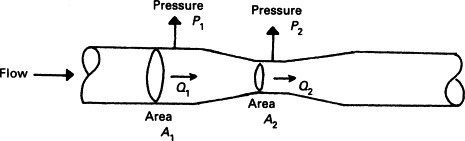
In Figure 6.1 the pipe is horizontal, so the potential energy is the same at all points. As the flow velocity increases through the restriction, the kinetic energy will increase and, for conservation of energy, the flow energy (i.e., the pressure) must fall.
This equation is the basis of all differential flowmeters.
Flow in a pipe can be smooth (called streamline or laminar) or turbulent. In the former case the flow velocity is not equal across the pipe being lower at the walls. With turbulent flow the flow velocity is equal at all points across a pipe. For accurate differential measurement the flow must be turbulent.
The flow characteristic is determined by the Reynolds number defined as
 where v is the fluid velocity, D the pipe diameter, ρ the fluid density, and η the fluid viscosity. Sometimes the kinematic viscosity ρ/η is used in the formula. The Reynolds number is a ratio and has no dimensions. If Re < 2000 the flow is laminar. If Re
> 105 the flow is fully turbulent.
where v is the fluid velocity, D the pipe diameter, ρ the fluid density, and η the fluid viscosity. Sometimes the kinematic viscosity ρ/η is used in the formula. The Reynolds number is a ratio and has no dimensions. If Re < 2000 the flow is laminar. If Re
> 105 the flow is fully turbulent.
Calculation of the actual pressure drop is complex, especially for compressible gases, but is generally of the form (6.1)
![]() where K is a constant for the restriction and ΔP the differential pressure. Methods of calculating K are given in British Standard BS 1042 and ISO 5167:1980. Computer programs can also be purchased.
where K is a constant for the restriction and ΔP the differential pressure. Methods of calculating K are given in British Standard BS 1042 and ISO 5167:1980. Computer programs can also be purchased.
The commonest differential pressure flow meter is the orifice plate shown in Figure 6.2. This is a plate inserted into the pipe with upstream tapping point at D and downstream tapping point at D/2 where D is the pipe diameter. The plate should be drilled with a small hole to release bubbles (liquid) or drain condensate (gases). An identity tag should be fitted showing the scaling and plant identification.
Figure 6.2. Mounting of an orifice pipe between flanges with D–D/2 tappings.

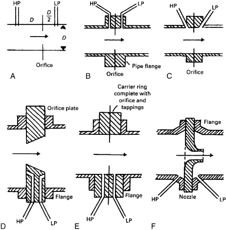
The D–D/2 tapping is the commonest, but other tappings shown in Figure 6.3 may be used where it is not feasible to drill the pipe.
Figure 6.3. Common methods of mounting orifice plates. (A) D–D/2, probably the commonest; (B) flange taps used on large pipes with substantial flanges; (C) corner taps drilled through flange; (D) plate taps, tappings built into the orifice plate; (E) orifice carrier, can be factory made and needs no drilling on site; (F) nozzle, gives smaller head loss.
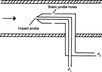
Orifice plates suffer from a loss of pressure on the downstream side (called the head loss). This can be as high as 50%. The venturi tube and Dall tube of Figure 6.4(B) have lower losses of around 5% but are bulky and more expensive. Another low-loss device is the pitot tube of Figure 6.5. Equation (6.1) applies to all these devices, the only difference being the value of the constant K.
Figure 6.4. Low-loss differential pressure primary sensors. Both give a much lower head loss than an orifice plate but at the expense of a great increase on pipe length. It is often impossible to provide the space for these devices, (A) venturi tube; (B) Dall tube.
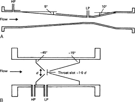
Figure 6.5. An insertion pitot tube.
Conversion of the pressure to an electrical signal requires a differential pressure transmitter and a linearizing square root unit. This square root extraction is a major limit on the turndown as zeroing errors are magnified. A typical turndown is 4:1.
The transmitter should be mounted with a manifold block as shown in Figure 6.6 to allow maintenance. Valves B and C are isolation valves. Valve A is an equalizing valve and is used, along with B and C, to zero the transmitter. In normal operation A is closed and B and C are open. Valve A should always be opened before valves B and C are closed prior to removal of the transducer to avoid high pressure being locked into one leg. Similarly on replacement valves B and C should both be opened before valve A is closed to prevent damage from the static pressure.
Figure 6.6. Connection of a differential pressure flow sensor such as an orifice plate to a differential pressure transmitter. Valves B and C are used for isolation and valve A for equalization.

Gas measurements are prone to condensate in pipes, and liquid measurements are prone to gas bubbles. To avoid these effects, a gas differential transducer should be mounted above the pipe and a liquid transducer below the pipe with tap off points in the quadrants.
Although the accuracy and turndown of differential flowmeters is poor (typically 4% and 4:1) their robustness, low cost, and ease of installation still makes them the commonest type of flowmeter.
6.3. Turbine Flowmeters
As its name suggests a turbine flowmeter consists of a small turbine placed in the flow as in Figure 6.7. Within a specified flow range (usually with about a 10:1 turndown for liquids 20:1 for gases), the rotational speed is directly proportional to flow velocity.
Figure 6.7. A turbine flowmeter. These are vulnerable to bearing failures if the fluid contains any solid particles.
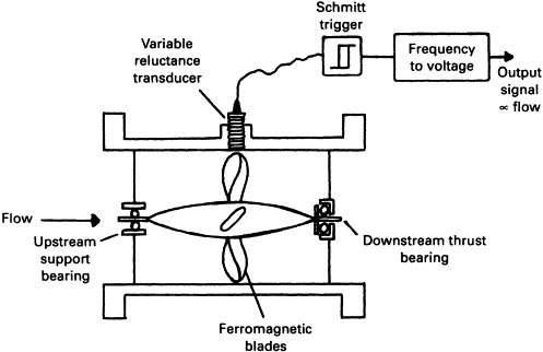
The turbine blades are constructed of ferromagnetic material and pass below a variable reluctance transducer producing an output approximating to a sine wave of the form
![]() where A is a constant, ω is the angular velocity (itself proportional to flow), and N is the number of blades. Both the output amplitude and the frequency are proportional to flow, although the frequency is
normally used.
where A is a constant, ω is the angular velocity (itself proportional to flow), and N is the number of blades. Both the output amplitude and the frequency are proportional to flow, although the frequency is
normally used.
The turndown is determined by frictional effects and the flow at which the output signal becomes unacceptably low. Other nonlinearities occur from the magnetic and viscous drag on the blades. Errors can occur if the fluid itself is swirling and upstream straightening vanes are recommended.
Turbine flowmeters are relatively expensive and less robust than other flowmeters. They are particularly vulnerable to damage from suspended solids. Their main advantages are a linear output and a good turndown ratio. The pulse output can also be used directly for flow totalization.
6.4. Vortex Shedding Flowmeters
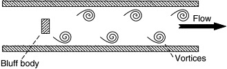
If a bluff (nonstreamlined) body is placed in a flow, vortices detach themselves at regular intervals from the downstream side as shown in Figure 6.8. The effect can be observed by moving a hand through water. In flow measurement the vortex shedding frequency is usually a few hundred hertz. Surprisingly at Reynolds numbers in excess of 103, the volumetric flow rate, Q, is directly proportional to the observed frequency of vortex shedding, f; that is,
![]() where K is a constant determined by the pipe and obstruction dimension.
where K is a constant determined by the pipe and obstruction dimension.
Figure 6.8. Vortex shedding flowmeter.
The vortices manifest themselves as sinusoidal pressure changes which can be detected by a sensitive diaphragm on the bluff body or by a downstream modulated ultrasonic beam.
The vortex shedding flowmeter is an attractive device. It can work at low Reynolds numbers, has excellent turndown (typically 15:1), no moving parts, and minimal head loss.
6.5. Electromagnetic Flowmeters
In Figure 6.9(A) a conductor of length l is moving with velocity v perpendicular to a magnetic field of flux density B. By Faraday's law of electromagnetic induction, a voltage E is induced where (6.2)
![]()
Figure 6.9. Electromagnetic flowmeter. (A) Electromagnetic induction in a wire moving in a magnetic field; (B) the principle applied with a moving conductive fluid.

This principle is used in the electromagnetic flowmeter. In Figure 6.9(B) a conductive fluid is passing down a pipe with mean velocity v through an insulated pipe section. A magnetic field B is applied perpendicular to the flow. Two electrodes are placed into the pipe sides to form, via the fluid, a moving conductor of length D relative to the field where D is the pipe diameter. From Equation (6.2) a voltage will occur across the electrodes that is proportional to the mean flow velocity across the pipe.
Equation (6.2) and Figure 6.9(B) imply a steady DC field. In practice an AC field is used to minimize electrolysis and reduce errors from DC thermoelectric and electrochemical voltages which are of the same order of magnitude as the induced voltage.
Electromagnetic flowmeters are linear and have an excellent turndown of about 15:1. There is no practical size limit and no head loss. They do, though, provide a few installation problems as an insulated pipe section is required, with earth bonding either side of the meter to avoid damage from any welding that may occur in normal service. They can only be used on fluids with a conductivity in excess of 1 mS m−1 which permits use with many (but not all) common liquids but prohibits their use with gases. They are useful with slurries with a high solids content.
6.6. Ultrasonic Flowmeters
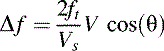
The Doppler effect occurs when there is relative motion between a sound transmitter and receiver as shown in Figure 6.10(A). If the transmitted frequency is ft Hz, Vs is the velocity of sound and V the relative velocity, the observed received frequency, ft will be
![]()
Figure 6.10. An ultrasonic flowmeter. (A) Principle of operation; (B) schematic of a clip on ultrasonic flowmeter.

A doppler flowmeter injects an ultrasonic sound wave (typically a few hundred kilohertz) at an angle θ into a fluid moving in a pipe as shown in Figure 6.10(B). A small part of this beam will be reflected back off small bubbles, solid matter, vortices, and the like and is picked up by a receiver mounted alongside the transmitter. The frequency is subject to two changes, one as it moves upstream against the flow, and one as it moves back with the flow. The received frequency is thus
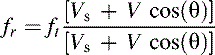 which can be simplified to
The doppler flowmeter measures mean flow velocity, is linear, and can be installed (or removed) without the need to break into the pipe. The turndown of about 100:1 is the best of all flowmeters. Assuming the measurement of mean flow velocity is acceptable, it can be used at all Reynolds numbers. It is compatible with all fluids and is well suited for difficult applications with corrosive liquids or heavy slurries.
6.7. Hot Wire Anemometer
If fluid passes over a hot object, heat is removed. It can be shown that the power loss is (6.3)
![]() where v is the flow velocity and A and B are constant. A is related to radiation and B to conduction.
where v is the flow velocity and A and B are constant. A is related to radiation and B to conduction.
Figure 6.11 shows a flowmeter based on Equation (6.3). A hot wire is inserted in the flow and maintained at a constant temperature by a self-balancing bridge. Changes in the wire temperature result in a resistance change which unbalances the bridge. The bridge voltage is automatically adjusted to restore balance.
Figure 6.11. The hot wire anemometer.
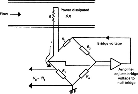
The current, l, though the resistor is monitored. With a constant wire temperature, the heat dissipated is equal to the power loss from which
![]()
Obviously the relationship is nonlinear, and correction will need to be made for the fluid temperature which will affect constants A and B.
6.8. Mass Flowmeters
The volume and density of all materials are temperature dependent. Some applications will require true volumetric measurements, some, such as combustion fuels, will really require mass measurement. Previous sections have measured volumetric flow. This section discusses methods of measuring mass flow.
The relationship between volume and mass depends on both pressure and absolute temperature (measured in kelvins). For a gas,
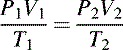
The relationship for a liquid is more complex, but if the relationship is known and the pressure and temperature are measured along with the delivered volume or volumetric flow, the delivered mass or mass flow rate can be easily calculated. Such methods are known as inferential flowmeters.
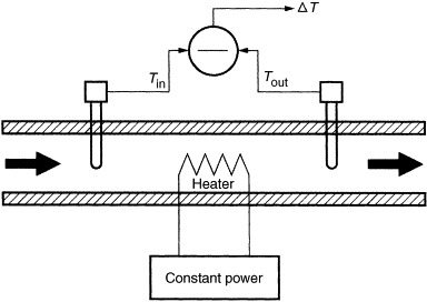
In Figure 6.12 a fluid is passed over an in-line heater with the resultant temperature rise being measured by two temperature sensors. If the specific heat of the material is constant, the mass flow, Fm, is given by
 where E is the heat input from the heater, Cp is the specific heat, and θ the temperature rise. The method is only suitable for relatively small flow rates.
Figure 6.12. Mass flow measurement by noting the temperature rise caused by a constant input power.
Many modern mass flowmeters are based on the Coriolis effect. In Figure 6.13 an object of mass m is required to move with linear velocity v from point A to point B on a surface that is rotating with angular velocity. If the object moves in a straight line as viewed by a static observer, it will appear to veer to the right when viewed by an observer on the disc.
Figure 6.13. Definition of Coriolis force.
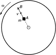
If the object is to move in a straight line as seen by an observer on the disc, a force must be applied to the object as it moves out. This force is known as the Coriolis force and is given by
![]() where m is the mass, ω is the angular velocity, and v the linear velocity. The existence of this force can be easily experienced by trying to move along a radius of a rotating
children's roundabout in a playground.
where m is the mass, ω is the angular velocity, and v the linear velocity. The existence of this force can be easily experienced by trying to move along a radius of a rotating
children's roundabout in a playground.
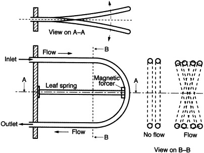
Coriolis force is not limited to pure angular rotation but also occurs for sinusoidal motion. This effect is used as the basis of a Coriolis flowmeter shown in Figure 6.14. The flow passes through a C-shaped tube which is attached to a leaf spring and vibrated sinusoidally by a magnetic forcer. The Coriolis force arises not, as might be first thought, because of the semicircle pipe section at the right-hand side but from the angular motion induced into the two horizontal pipe sections with respect to the fixed base. If there is no flow, the two pipe sections will oscillate together. If there is flow, the flow in the top pipe is in the opposite direction to the flow in the bottom pipe and the Coriolis force causes a rolling motion to be induced as shown. The resultant angular deflection is proportional to the mass flow rate.
Figure 6.14. Simple Coriolis mass flowmeter. A multiturn coil is often used in place of the C segment.
The original meters used optical sensors to measure the angular deflection. More modern meters use a coil rather than a C section and sweep the frequency to determine the resonant frequency. The resonant frequency is then related to the fluid density by
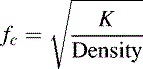 where K is a constant. The mass flow is determined either by the angular measurement or the phase shift in velocity. Using the resonant
frequency maximizes the displacement and improves measurement accuracy.
where K is a constant. The mass flow is determined either by the angular measurement or the phase shift in velocity. Using the resonant
frequency maximizes the displacement and improves measurement accuracy.
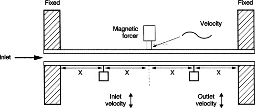
Coriolis measurement is also possible with a straight pipe. In Figure 6.15 the center of the pipe is being deflected with a sinusoidal displacement and the velocity of the inlet and outlet pipe sections monitored. The Coriolis effect will cause a phase shift between inlet and outlet velocities. This phase shift is proportional to the mass flow.
Figure 6.15. Vibrating straight pipe mass flowmeter.