
Chapter 7. Temperature
Temperature is one of the most important parameters in process control. Accurate measurement of the temperature is not easy and to obtain accuracies better than 0.5° C great care is needed. Errors occur due to several sources, such as the sensor nonlinearities, temperature gradients, calibration errors, and poor thermal contact.
This chapter describes the temperature scales and the types of sensors and their comparisons.
7.1. Temperature Scales
The unit of the fundamental physical quantity known as the thermodynamic temperature (unit T) is the kelvin, symbol K, defined as the fraction 1/273.15 of the thermodynamic temperature of the triple point of water. Most people think in terms of degrees Celsius. The relation between kelvins and Celsius is (7.1)
![]() From Equation (7.1) it is clear that the triple point of water in degrees Celsius is 0.01° C. From a practical point of view, the ice point is
0° C, and the steam point 100° C. Table 7.1 gives the fixed temperature points of some commonly known physical phenomena.
From Equation (7.1) it is clear that the triple point of water in degrees Celsius is 0.01° C. From a practical point of view, the ice point is
0° C, and the steam point 100° C. Table 7.1 gives the fixed temperature points of some commonly known physical phenomena.
Table 7.1. Some commonly known temperature points
| Scale | Absolute zero | Ice point | Water boiling point |
|---|---|---|---|
| Celsius, ° C | −273.15 | 0 | 100 |
| Fahrenheit, °F | −459.67 | 32 | 212 |
| Kelvin, K | 0 | 273.15 | 373.15 |
On January 1, 1990, a new temperature scale was introduced, known as the International Temperature Scale of 1990 (ITS-90). This scale supersedes the Microcontroller-Based Temperature Monitoring and Control International Practical Temperature Scale of 1968 (amended edition of 1975). The new ITS-90 scale resulted in changes of 1.5° C at 3000° C and less than 0.025° C between −100° C to +100° C. For the people who are interested in precision temperature measurement, these changes may be significant, but for most temperature applications, these changes are not important. Table 7.2 shows the fixed points adopted in ITS-90. The ITS-90 extends upwards from 0.65K to the highest temperature practically measurable. It comprises a number of ranges and subranges and several of these ranges or subranges overlap. The melting and freezing point measurements are conducted at a pressure of 101.325 kPa.
Table 7.2. Fixed points adopted in ITS-90
| Material | Measurement point | Temperature (t90/K) | Temperature (t90/° C) |
|---|---|---|---|
| Hydrogen | Triple point | 13.8033 | −259.3467 |
| Hydrogen | Boiling point at 33,321.3 Pa | 17.035 | −256.115 |
| Hydrogen | Boiling point at 101,292 Pa | 20.27 | −252.88 |
| Neon | Triple point | 24.5561 | −248.5939 |
| Oxygen | Triple point | 54.3584 | −218.7916 |
| Argon | Triple point | 83.8058 | −189.3442 |
| Mercury | Triple point | 234.3156 | −38.8344 |
| Water | Triple point | 273.16 | 0.01 |
| Gallium | Melting point | 302.9146 | 29.7646 |
| Indium | Freezing point | 429.7485 | 156.5985 |
| Tin | Freezing point | 505.078 | 231.928 |
| Zinc | Freezing point | 692.677 | 419.527 |
| Aluminum | Freezing point | 933.473 | 660.323 |
| Silver | Freezing point | 1234.93 | 961.78 |
| Gold | Freezing point | 1337.33 | 1064.18 |
| Copper | Freezing point | 1357.77 | 1084.62 |
7.2. Types of Temperature Sensors
There are many types of sensors to measure the temperature. Some sensors such as the thermocouples, RTDs, and thermistors are the older classical sensors and they are used extensively due to their big advantages. The new generation of sensors such as the integrated circuit sensors and radiation thermometry devices are popular only for limited applications.
The choice of a sensor depends on the accuracy, the temperature range, speed of response, thermal coupling, the environment (chemical, electrical, or physical), and the cost.
As shown in Table 7.3, thermocouples are best suited to very low and very high temperature measurements. The typical measuring range is −270° C to +2600° C. Thermocouples are low cost and very robust. They can be used in most chemical and physical environments. External power is not required to operate them and the typical accuracy is ±1° C.
Table 7.3. Temperature sensors
| Sensor | Temperature range, ° C | Accuracy, ±° C | Cost | Robustness |
|---|---|---|---|---|
| Thermocouple | −270 to +2600 | 1 | Low | Very high |
| RTD | −200 to +600 | 0.2 | Medium | High |
| Thermistor | −50 to +200 | 0.2 | Low | Medium |
| Integrated circuit | −40 to +125 | 1 | Low | Low |
RTDs are used in medium-range temperatures, ranging from −200° C to +600° C. They offer high accuracy, typically ±0.2° C. RTDs can usually be used in most chemical and physical environments, but they are not as robust as the thermocouples. The operation of RTDs require external power.
Thermistors are used in low- to medium-temperature applications, ranging from −50° C to +200° C. They are not as robust as the thermocouples or the RTDs and they can not easily be used in chemical environments. Thermistors are low cost and their accuracy is around ±0.2° C.
Semiconductor sensors are used in low-temperature applications, ranging from −40° C to about +125° C. Their thermal coupling with the environment is not very good and the accuracy is around ±1° C. Semiconductors are low cost and some models offer digital outputs, enabling them to be directly connected to computer fduipment without the need of A/D converters.
Radiation thermometry devices measure the radiation emitted by hot objects, based upon the emissivity of the object. But the emissivity is usually not known accurately, and additionally it may vary with time, making accurate conversion of radiation to temperature difficult. Also, radiation from outside the field of view may enter the measuring device, resulting in errors in the conversion. Radiation thermometry devices have the advantages that they can be used to measure temperatures in a wide range (450° C to 2000° C) with an accuracy better than 0.5%. Radiation thermometry requires special signal processing hardware and software and is not covered in this book.
The advantages and disadvantages of various types of temperature sensors are given in Table 7.4.
Table 7.4. Comparison of temperature sensors
| Sensor | Advantages | Disadvantages |
|---|---|---|
| Thermocouple | Wide operating temperature range | Nonlinear |
| Low cost | Low sensitivity | |
| Rugged | Reference junction compensation required | |
| Subject to electrical noise | ||
| RTD | Linear | Slow response time |
| Wide operating temperature range | Expensive | |
| High stability | Current source required | |
| Sensitive to shock | ||
| Thermistor | Fast response time | Nonlinear |
| Low cost | Current source required | |
| Small size | Limited operating temperature range | |
| Large change in resistance vs. temperature | Not easily interchangeable without recalibration | |
| Integrated circuit | Highly linear | Limited operating temperature range |
| Low cost | Voltage or current source required | |
| Digital output sensors can be directly connected to a microprocessor without an A/D converter | Self-heating errors | |
| Not good thermal coupling with the environment |
Example 7.1
It is required to measure the melting point of a chemical substance that is known to be between 1500° C and 1800° C. What type of temperature sensor would you choose?
Solution 7.1
The only sensor that can work at the required temperatures is a thermocouple. Care should be taken to ensure that the chosen thermocouple is suitable for the chemical environment.
Example 7.2
It is required to measure the temperature of a gas to an accuracy of around a few degrees. The temperature of the gas is between 0° C and +50° C. What type of temperature sensor would you choose?
Solution 7.2
Most sensors can be used for this purpose but probably the best choice would be to use a low-cost semiconductor-type sensor.
7.3. Measurement Errors
There could be several sources of errors during the measurement of temperature. Some important errors are described in this section.
7.3.1. Calibration Errors
Calibration errors can occur as a result of offset and linearity errors. These errors can drift with aging and temperature cycling. It is recommended by the manufacturers to calibrate the measuring fduipment from time to time. Sensor interchangeability is also an important criterion. This refers to the maximum likely error to occur after replacing a sensor with another of the same type without recalibrating. RTDs are considered to be the most accurate and stable sensors.
7.3.2. Sensor Self-Heating
RTDs, thermistors, and semiconductor sensors require an external power supply so that a reading can be taken. This external power can cause the sensor to heat, causing an error in the reading. The effect of self-heating depends on the size of the sensor and the amount of power dissipated by the sensor. Self-heating can be avoided by using the lowest possible external power or by calibrating the self-heating into the measurement.
7.3.3. Electrical Noise
Electrical noise can introduce errors into the measurement. Thermocouples produce extremely low voltages, and as a result of this, noise can easily enter into the measurement. This noise can be minimized by using low-pass filters, avoiding ground loops, and keeping the sensors and the lead wires away from electrical machinery.
7.3.4. Mechanical Stress
Some sensors such as the RTDs are sensitive to mechanical stress and can give wrong outputs when subjected to stress. Mechanical stress can be minimized by avoiding the deformation of the sensor, by not using adhesives to fix a sensor to a surface, and by using sensors such as thermocouples which are less sensitive to mechanical stress.
7.3.5. Thermal Coupling
It is important that the sensor used makes a good thermal contact with the measuring surface. If the surface has a thermal gradient (e.g., as a result of poor thermal conductivity), then the placement of the sensor should be chosen with care. If the sensor is used in a liquid, the liquid should be stirred to cause a uniform heat distribution. Semiconductor sensors usually suffer from good thermal contact since they are not easily mountable to the surface whose temperature is to be measured.
7.3.6. Sensor Time Constant
This can be another source of error. Every type of sensor has a time constant such that it takes time for a sensor to respond to a change in the external temperature. The time constant is defined as the time it takes for the output to reach 63% of its final steady-state value. Errors due to the sensor time constant can be minimized by improving the thermal coupling or by using a sensor with a small time constant.
7.3.7. Sensor Leads
Sensor leads are usually copper and therefore they are excellent heat conductors. These wires can lead to errors in measurements if placed in an environment with a temperature different from the measured surface temperature. These errors can be minimized by using thin wires or by taking care in placing the lead wires.
7.4. Selecting a Temperature Sensor
Selecting the appropriate sensor is not always easy. This depends on factors such as the temperature range, required accuracy, environment, speed of response, ease of use, cost, interchangeability, and so on. Traditionally, thermocouples are used in high-temperature chemical industries such as glass and plastic processes. Environmental applications, electronics hobby market, and automotive industries generally use thermistors or integrated circuit sensors. RTDs are commonly used in lower-temperature, higher-precision chemical industries.
7.5. Thermocouple Temperature Sensors
Thermocouples are simple temperature sensors consisting of two dissimilar metals joined together. In 1821 a German physicist named Thomas Seeback discovered that thermoelectric voltage is produced and an electric current flows in a closed circuit of two dissimilar metals if the two junctions are held at different temperatures. As shown in Figure 7.1, one of the junctions is designated the hot junction and the other junction is designated as the cold or reference junction. The current developed in the closed loop is proportional to the types of metals used and the difference in temperature between the hot and the cold junctions.
Figure 7.1. A thermocouple circuit.

If the same temperature exists at both junctions, the voltages produced cancel each other out and no current flows in the circuit. A thermocouple therefore measures the temperature difference between the two junctions and not the absolute temperature.
In order to measure the temperature, we have to insert a voltage measuring device in the loop to measure the thermoelectric effect. Figure 7.2 shows such an arrangement where the measurement device is connected to the thermocouple with a pair of copper wires, using a terminal block.
Figure 7.2. Connecting a measurement device.
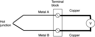
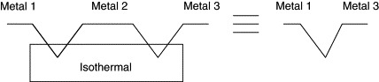
Thermocouple wires are usually different metals from the measuring device wires, and as a result, an additional pair of thermocouples are formed at the connection points. Figure 7.3 shows these additional undesirable thermocouples as junction 2 and junction 3. Although these additional thermocouples seem to cause a problem, the application of the law of intermediate metals shows that these thermocouples will have no effect if they are kept at the same temperature. The law of intermediate metals simply states that a third metal may be inserted into a thermocouple system without affecting the system if the junctions with the third metal are kept isothermal (i.e., at the same temperature). Figure 7.4 illustrates the principle of the law of intermediate metals.
Figure 7.3. Additional thermocouples at junction 2 and junction 3.

Figure 7.4. The law of intermediate metals.
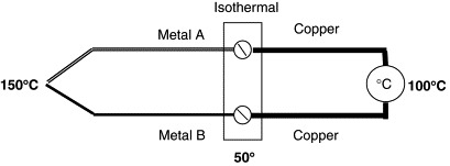
Thus, if junction 2 and junction 3 are kept at the same temperatures, the voltage measured by the voltmeter will be proportional to the difference in temperature between junction 1 (hot junction) and junctions 2 and 3. This is illustrated in Figure 7.5 where the junction temperature is at 150° C and the terminal block is kept at 50° C. The measured temperature is then the difference, that is, 100° C. Junction 1 is the hot junction and the temperature of the terminal block is the temperature of the cold junction.
Figure 7.5. Thermocouple with isothermal terminal block.
Thermocouples produce a voltage that is proportional to the difference in temperature between the hot and the cold (or the reference) junctions. If we want to know the absolute temperature of the hot junction, first we have to know the absolute temperature of the reference junction. If the reference junction is known and is controlled and stable, then there is no problem. If the temperature of the reference junction is not known, one of the following methods can be used:
- Measure the temperature of the reference junction accurately and use this value to calculate the temperature of the hot junction. The simplest method to measure the temperature of the reference junction is to use a thermistor or a semiconductor temperature sensor. Then, the temperature of the reference junction should be added to the measured thermocouple temperature (see Figure 7.5). This method gives accurate results and the cost is generally low.
- Locate the reference junction in a thermally controlled environment where the temperature is known accurately. For example,
as shown in Figure 7.6, an ice bath can be used to keep the reference junction at the ice temperature. Notice here that the reference junction is
moved from the terminal block by inserting a metal A into the measurement system. Alternatively, we could just immerse the terminal block into the ice, but this is not very practical.
Ice bath compensation gives very accurate results but generally they are not very practical in industrial applications.
Figure 7.6. Using an ice bath for the reference junction.

- Do not use copper wires for the measurement device, but extend the thermocouple wires right into the measurement device. Connect to the copper wires inside the measurement device where the reference junction temperature can easily and accurately be measured.
- Use cold junction compensating ICs, such as the Linear Technology LT1025. These ICs have built-in temperature sensors that detect the temperature of the reference junction. The IC then produces a voltage that is proportional to the voltage produced by a thermocouple with its hot junction at the ambient temperature and its cold junction at 0° C. This voltage is added to the voltage produced by the thermocouple and the net effect is as if the reference junction is kept at 0° C. Cold junction compensating ICs are accurate to a few degrees Celsius and they are used very commonly in many applications that do not require precision measurements.
7.5.1. Thermocouple Types
There are about 12 standard thermocouple types that are commonly used. Each type is given an internationally approved letter that indicates the materials that the thermocouple is manufactured from. Table 7.5 shows the most popular thermocouples, their materials, and the usable temperature ranges.
Table 7.5. Popular thermocouples
| Type | +Lead | −Lead | Seeback coefficient (μV/° C) | Temperature range (° C) |
|---|---|---|---|---|
| K | Ni + 10%Cr | Ni + 2%Al + 2%Mn + 1%Si | 42 | −180 to +1350 |
| J | Fe | Cu +43%Ni | 54 | −180 to +750 |
| N | Ni + 14%Cr + 1.5%Si | Ni + 4.5%Si + 0.1%Mg | 30 | −270 to +1300 |
| T | Cu | Cu +43%Ni | 46 | −250 to +400 |
| E | Ni + 10%Cr | Cu +43%Ni | 68 | −40 to +900 |
| R | Pt + 13%Rh | Pt | 8 | −50 to +1700 |
| B | Pt + 30%Rh | Pt + 6%Rh | 1 | +100 to +1750 |
Type K
Type K thermocouple is constructed using Ni-Cr (called Chromel), and Ni-Al (called Alumel) metals. It is low cost and one of the most popular general purpose thermocouples. The operating range is around −180° C to +1350° C. Sensitivity is approximately 42 μV/° C. Type K is most suited to oxidizing environments.
Type J
Constructed from iron and Cu-Ni metals, the temperature range of this thermocouple is −180° C to +750° C. As a result of the risk of iron oxidization, this thermocouple is used in plastic molding industry. The sensitivity of type J thermocouple is 54 μV/° C. Type J thermocouple is generally recommended for new designs.
Type N
Type N thermocouple is constructed from Ni-Cr-Si (Nicrosil) and Ni-Si-Mg (Nisil) metals. The temperature range is −270° C to +1300° C. The sensitivity of type N is 30 μV/° C and it is generally used at high temperatures.
Type T
Type T thermocouple is constructed from Cu and Cu-Ni. The operating temperature range is −250° C to +400° C. This thermocouple is relatively low cost and is suited to low-temperature applications. The sensitivity of this thermocouple is 46 μV/° C. Type T is tolerant to moisture.
Type E
Type E thermocouple is constructed using Ni-Cr (Chromel) and Cu-Ni (constantan) metals. The temperature range is −40° C to +900° C. This thermocouple has the highest sensitivity at 68 μV/° C and it can be used in the vacuum and in unprotected sensor applications.
Type R
Type R is constructed using Pt-Rh (platinum-radium) and Pt (platinum). The sensitivity is low at 8 μV/° C. The temperature range of this thermocouple is −50° C to +1700° C. Type R is used to measure very high temperatures. Since it can easily be contaminated, it normally requires protection.
Type B
Type B thermocouple is constructed using Pt-Rh (platinum-radium) metals with different compositions. The sensitivity is very low, at 1 μV/° C, and the temperature range is −100° C to +1750° C. Type B is used at measuring high temperatures, such as in the glass industry.
Thermocouples are usually identified by color codes. Unfortunately, there is no standard single color code and different countries have adopted different codes. For example, the American standard identifies the positive leg of a type K thermocouple with the yellow color and the negative leg with the red color.
7.6. RTD Temperature Sensors
7.6.1. RTD Principles
The term RTD is short for resistance temperature detector. The RTD is a temperature-sensing device whose resistance increases with temperature. RTDs are quite linear devices and a typical temperature–resistance characteristic is shown in Figure 7.7. RTDs operate on the principle that the electrical resistance of metals change with temperature. Although in theory any kind of metal can be used for temperature sensing, in practice metals with high melting points that can withstand the effects of corrosion and those with high resistivities are chosen. Table 7.6 gives the resistivities of some commonly used RTD metals. Gold and silver have low resistivities and as a result their resistances are relatively low, making the measurement difficult. Copper has low resistivity but is sometimes used because of its low cost. The most commonly used RTDs are made of either nickel, platinum, or nickel alloys. Nickel sensors are used in cost-sensitive applications such as consumer goods and they have a limited temperature range. Nickel alloys, such as nickel-iron, is lower in cost than the pure nickel and in addition it has a higher operating temperature. Platinum is by far the most common RTD material, mainly because of its high resistivity and long-term stability in air.
Figure 7.7. Typical RTD temperature–resistance characteristics.
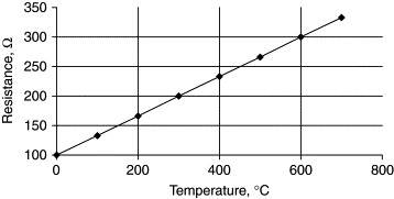
Table 7.6. Resistivities and temperature ranges of same RTD metals
| Metal | Resistivity (Ω/cmf) |
|---|---|
| Silver | 8.8 |
| Copper | 9.26 |
| Gold | 13.00 |
| Tungsten | 30.00 |
| Nickel | 36.00 |
| Platinum | 59.00 |
RTDs have excellent accuracies over a wide temperature range and some RTDs have accuracies better than 0.001° C. Another advantage of the RTDs is that they drift less than 0.1° C/year.
If the same temperature exists at both junctions, the voltages produced cancel each other out and no current flows in the circuit. A thermocouple therefore measures the temperature difference between the two junctions and not the absolute temperature.
RTDs are difficult to measure because of their low resistances and only slight changes with temperature, usually on the order of 0.40/° C. To accurately measure such small changes in resistance, special circuit configurations are usually needed. For example, long leads could cause errors as they introduce extra resistance to the circuit.
RTDs are resistive devices and a current must pass through the device so that the voltage across the device can be measured. This current can cause the RTD to self-heat and consequently it can introduce errors into the measurement. Self-heating can be minimized by using the smallest possible excitation current. The amount of self-heating also depends on where and how the sensor is used. An RTD can self-heat much quicker in still air than in a moving liquid.
7.6.2. RTD Types
In order to achieve high stability and accuracy, RTD sensors must be contamination free. Below about 250° C the contamination is not much of a problem, but above this temperature, special manufacturing techniques are used to minimize the contamination of the RTD element.
The RTD sensors are usually manufactured in two forms: wire wound or thin film. Figure 7.8 shows a typical RTD sensor. Wire wound RTDs are made by winding a very fine strand of platinum wire into a coil shape around a nonconducting material (e.g., ceramic or glass) until the required resistance is obtained. The assembly is then treated to protect against short-circuit and to provide vibration resistance. Although the wire wound RTDs are very stable, the thermal contact between the platinum and the measured point is not very good and results in slow thermal response. Thin film RTDs are made by depositing a layer of platinum in a resistance pattern on a ceramic substrate. The film is treated to have the required resistance and then coated with glass or epoxy for moisture resistance and to provide vibration resistance. Thin film RTDs have the advantages that they provide a fast thermal response, are less sensitive to vibration, and they cost less than their wire wound counterparts. Thin film RTDs can also provide a higher resistance for a given size. These RTDs are less stable than the wire wound ones but they are becoming very popular as a result of their considerably lower costs.
Figure 7.8. A typical RTD sensor.

7.6.3. RTD Temperature–Resistance Relationship
Every metal has a resistance and this resistance is directly proportional to length and the resistivity of the metal and inversely proportional to its cross-sectional area: (7.2)
![]() where R is the resistance of the metal, ρ is the resistivity, L is the length of the metal, and A is the cross-sectional area of the metal.
where R is the resistance of the metal, ρ is the resistivity, L is the length of the metal, and A is the cross-sectional area of the metal.
The resistivity increases with increasing temperature as shown in Equation (7.3): (7.3)
![]() where ρt is the resistivity at temperature t, ρ0 is the resistivity at a standard temperature t0, and a is the temperature coefficient of resistance.
where ρt is the resistivity at temperature t, ρ0 is the resistivity at a standard temperature t0, and a is the temperature coefficient of resistance.
Setting t0 to 0° C, we can rewrite Equation (7.3) as (7.4)
![]() If R0 is the resistance at 0° C and Rt is the resistance at temperature t, we can rewrite Equation (7.2) as (7.5)
If R0 is the resistance at 0° C and Rt is the resistance at temperature t, we can rewrite Equation (7.2) as (7.5)
![]() and (7.6)
and (7.6)
![]() or, from Equations (7.4) and (7.6), (7.7)
or, from Equations (7.4) and (7.6), (7.7)
![]() and using Equations (7.5) and (7.7), we can write the relationship between the temperature and the resistance as (7.8)
and using Equations (7.5) and (7.7), we can write the relationship between the temperature and the resistance as (7.8)
![]() Equation (7.8) is a simplified model of the RTD temperature–resistance relationship. In practice, the temperature–resistance relationship
of the RTDs are approximated by an fduation known as the Callendar–Van Dusen fduation which gives very accurate results. This fduation has the form (7.9)
Equation (7.8) is a simplified model of the RTD temperature–resistance relationship. In practice, the temperature–resistance relationship
of the RTDs are approximated by an fduation known as the Callendar–Van Dusen fduation which gives very accurate results. This fduation has the form (7.9)
![]() where A, B, and C are constants that depend upon the material. Above 0° C, the constant C is fdual to zero and we can rewrite Equation (7.9) as (7.10)
where A, B, and C are constants that depend upon the material. Above 0° C, the constant C is fdual to zero and we can rewrite Equation (7.9) as (7.10)
![]()
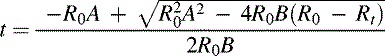
Thus, if we know the constants A and B and the resistance at 0° C, then we can calculate the resistance at any other positive temperature using Equation (7.10). However, in practice it is required to calculate the temperature from a knowledge of the RTD resistance. Equation (7.10) is a quadratic fduation in t and it can be solved to give (7.11)
An example is given next to illustrate the steps in calculating the temperature.
Example 7.3
The resistance of an RTD is 100Ω at 0° C. If the A and B constants are as given here, calculate the temperature when the resistance is measured as 138Ω.
![]()
![]()
![]()
![]()
![]()
Solution 7.3
The temperature can be calculated using Equation (7.11).
![]() which gives
which gives
![]()
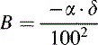
Some manufacturers provide RTD constants known as α, β, and δ. Knowing these constants, we can calculate the standard A, B, and C constants as (7.12)
![]() (7.13)
(7.13)
 (7.14)

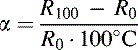
Parameter α is important as it is used in defining the RTD standards. This parameter is the change in RTD resistance from 0° C to 100° C, divided by the resistance at 0° C, divided by 100° C. Thus, α represents the mean resistance change referred to the nominal resistance at 0° C: (7.15)
Example 7.4
The α, β, and δ constants of a platinum RTD used to measure the temperature between 0° C and 80° C are specified by the manufacturers as
![]()
![]()
![]()
Calculate the standard RTD constants A, B, and C.
Solution 7.4
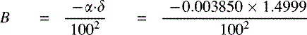
From Equations (7.12) and (7.13),
![]() or
or
![]() and
and
 or
or
![]()
![]() since the RTD is used to measure positive temperatures.
since the RTD is used to measure positive temperatures.
7.6.4. RTD Standards
Platinum RTDs conform to either IEC/DIN standard or reference-grade standards. The main difference is in the purity of the platinum used. The IEC/DIN standard defines pure platinum which is contaminated with other platinum group metals. The reference-grade platinum is made from 99.99% pure platinum.
The most commonly used international RTD standard is the IEC 751. Other international standards such as BS 1904 and DIN 43760 match this standard. IEC 751 is based on platinum RTDs with a resistance of 100Ω at 0° C and a parameter of 0.00385. Two performance classes are defined under the IEC 751: Class A and Class B. These performance classes, also known as DIN A and DIN B (due to DIN 43760), define tolerances on ice point and temperature accuracy.
The Callendar–Van Dusen parameters of IEC 751 standard RTDs are as follows:
![]()
![]()
![]()
Table 7.7 lists the properties of both classes. The temperature and resistance tolerances are listed in Tables 7.8 and 7.9, respectively. These tolerances are also plotted in Figures 7.9 and 7.10.
Table 7.7. IEC 751 RTD class properties
| Parameter | IEC 751 Class A | IEC 751 Class B |
|---|---|---|
| R0 | 100Ω ± 0.06% | 100Ω ± 0.12% |
| Alpha, α | 0.00385 ± 0.000063 | 0.00385 ± 0.000063 |
| Range | −200° C to 650° C | −200° C to 850° C |
| Temperature tolerance | ±(0.15 + 0.002∣T∣)° C | ±(0.3 + 0.005∣T∣)° C |
Table 7.8. Temperature tolerances of IEC 751 RTD sensors
| Temperature (° C) | IEC 751 Tolerance | |
|---|---|---|
| Class A (±° C) | Class B (±° C) | |
| −200 | 0.55 | 1.3 |
| −100 | 0.35 | 0.8 |
| 0 | 0.15 | 0.3 |
| 100 | 0.35 | 0.8 |
| 200 | 0.55 | 1.3 |
| 300 | 0.75 | 1.8 |
| 400 | 0.95 | 2.3 |
| 500 | 1.15 | 2.8 |
| 600 | 1.35 | 3.3 |
| 650 | 1.45 | 3.6 |
| 700 | — | 3.8 |
| 800 | — | 4.3 |
| 850 | — | 4.6 |
Table 7.9. Resistance tolerances of IEC 751 RTD sensors
| Temperature (° C) | IEC 751 Tolerance | |
|---|---|---|
| Class A (±°Ω) | Class B (±°Ω) | |
| −200 | 0.24 | 0.56 |
| −100 | 0.14 | 0.32 |
| 0 | 0.06 | 0.12 |
| 100 | 0.13 | 0.30 |
| 200 | 0.20 | 0.48 |
| 300 | 0.27 | 0.64 |
| 400 | 0.33 | 0.79 |
| 500 | 0.38 | 0.93 |
| 600 | 0.43 | 1.06 |
| 650 | 0.46 | 1.13 |
| 700 | — | 1.17 |
| 800 | — | 1.28 |
| 850 | — | 1.34 |
Figure 7.9. IEC 751 RTD temperature tolerances.

Figure 7.10. IEC 751 RTD resistance tolerances.

7.6.4.1. Class A Standard
This standard defines the temperature within the range −200° C to +650° C. The resistance at 0° C is R0 = 100Ω, and at 100° C it is R100 = 138.5Ω. Class A temperature tolerance is
![]() where ∣t∣ is the absolute value of the temperature in degrees Celsius; for example, at 0° C the temperature tolerance is ±0.15° C.
where ∣t∣ is the absolute value of the temperature in degrees Celsius; for example, at 0° C the temperature tolerance is ±0.15° C.
7.6.4.2. Class B Standard
Class B provides less accuracy than Class A. This standard defines the temperature within the range −200° C to +850° C. The resistance at 0° C is R0 = 100Ω, and at 100° C it is R100 = 138.5Ω. Class B temperature tolerance is
![]()
For example, at 0° C the temperature tolerance is ±0.3° C.
7.6.5. Practical RTD Circuits
Platinum RTDs are very low-resistance devices and they produce very little resistance changes for large temperature changes. For example, a 1° C temperature change will cause a 0.384-Ω change in resistance, so even a small error in measurement of the resistance can cause a large error in the measurement of the temperature. For example, consider a 100-Ω RTD with a 1-mA excitation current. If the temperature rises by 1° C, the voltage across the RTD will increase by only about 0.5 mV. If the excitation current is 100 mA, the same change in temperature will result in a 50-mV change in the voltage, which is much easier to measure accurately. A high-excitation current however should be avoided since it could give rise to self-heating of the sensor. The resistance of the wires leading to the sensor could give rise to errors when long wires are used. RTDs are usually used in bridge circuits for precision temperature measurement applications. Various practical RTD circuits are given in this section.
7.6.5.1. Simple Current Source Circuit
Figure 7.11 shows a simple RTD circuit where a constant current source I is used to pass a current through the RTD. The voltage across the RTD is measured and then the resistance of the RTD is calculated. The temperature can then be found by using Equation (7.15). This circuit has the disadvantage that the resistance of the wires could add to the measured resistance and hence it could cause errors in the measurement. For example, a lead resistance of 0.3Ω in each wire adds 0.6Ω error to the resistance measurement. For a platinum RTD with a = 0.00385, this resistance is fdual to 0.6Ω/(0.385Ω/° C) = 1.6° C error. Care should also be taken not to pass a large current through the RTD since this can cause self-heating of the RTD and hence change of its resistance. For example, a current of 1 mA through a 100-Ω RTD will generate 100 μW of heat. If the sensor element is unable to dissipate this heat, it will cause the resistance of the element to increase and hence an artificially high temperature will be reported.
Figure 7.11. Simple current source RTD circuit.
7.6.5.2. Simple Voltage Source Circuit
Figure 7.12 shows how an excitation current can be passed through an RTD by using a constant voltage source. This circuit suffers from the same problems as the one in Figure 7.11. The voltage across the RTD element is (7.16)
 and the resistance of the RTD element can be calculated as (7.17)
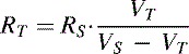
Figure 7.12. Simple voltage source RTD circuit.

7.6.5.3. Four-Wire RTD Measurement
When long leads are used (e.g., greater than about 5 m), it is necessary to compensate for the resistance of the lead wires. In the four-wire measurement method (see Figure 7.13), one pair of wires carries the current through the RTD, the other pair senses the voltage across the RTD. In Figure 7.12, RL1 and RL4 are the lead wires carrying the current and RL2 and RL3 are the lead wires for measuring the voltage across the RTD. Since only negligible current flows through the sensing wires (the voltage measurement device having a very high internal resistance), the lead resistances RL2 and RL3 can be neglected. Four-wire RTD measurement gives very accurate results and is the preferred method for accurate, precision RTD temperature measurement applications.
Figure 7.13. Four-wire RTD circuit.

7.6.5.4. Simple RTD Bridge Circuit
As shown in Figure 7.14, a simple Wheatstone bridge circuit can be used with the RTD at one of the legs of the bridge. As the temperature changes so does the resistance of the RTD and the output voltage of the bridge. This circuit has the disadvantage that the lead resistances RL1 and RL2 add to the resistance of the RTD, giving an error in the measurement.
Figure 7.14. Simple RTD bridge circuit.
7.6.5.5. Three-Wire RTD Bridge Circuit
As shown in Figure 7.15, RL1 and RL3 carry the bridge current. When the bridge is balanced, no current flows through RL2 and thus the lead resistance RL2 does not introduce any errors into the measurement. The effects of RL1 and RL3 at different legs of the bridge cancel out since they have the same lengths and are made up of the same material.
Figure 7.15. Three-Wire RTD bridge circuit.

7.6.6. Microcontroller-Based RTD Temperature Measurement
RTDs give analog output voltages and the measured temperature can simply be displayed using an analog meter (e.g., a voltmeter). Although this may be acceptable for some applications, accurate temperature measurement and display require digital techniques.
Figure 7.16 shows how the temperature can be measured using an RTD and a microcontroller. The temperature is sensed by the RTD and a voltage is produced that is proportional to the measured temperature. This voltage is filtered using a low-pass filter to remove any unwanted high-frequency noise components. The output of the filter is then amplified using an operational amplifier so that this output can be fed to an A/D converter. The digitized voltage is then read by the microcontroller and the resistance of the RTD is calculated. After this, the measured temperature can be calculated using Equation (7.11). Finally, the temperature is displayed on a suitable digital display (e.g., an LCD).
Figure 7.16. Microcontroller-based RTD temperature measurement.
![]()
7.7. Thermistor Temperature Sensors
7.7.1. Thermistor Principles
The name thermistor derives from the words thermal and resistor. Thermistors are temperature-sensitive passive semiconductors that exhibit a large change in electrical resistance when subjected to a small change in body temperature. As shown in Figure 7.17 thermistors are manufactured in a variety of sizes and shapes. Beads, discs, washers, wafers, and chips are the most widely used thermistor sensor types.
Figure 7.17. Some typical thermistors.

Disc thermistors are made by blending and compressing various metal oxide powders with suitable binders. The discs are formed by compressing under very high pressure on pelleting machines to produce round, flat ceramic bodies. An electrode material (usually silver) is then applied to the opposite sides of the disc to provide the contacts for attaching the lead wires. Sometimes a coating of glass or epoxy is applied to protect the devices from the environment and mechanical stresses. Finally, the thermistors are subjected to a special aging process to ensure high stability of their values. Typical coated thermistors measure 2.0 mm to 4.0 mm in diameter.
Washer-shaped thermistors are a variation of the standard disc shaped thermistors, and they usually have a hole in the middle so that they can easily be connected to an assembly.
Bead thermistors have lead wires that are embedded in the ceramic material. They are manufactured by combining the metal oxide powders with suitable binders and then firing them in a furnace with the leads on. After firing, the ceramic body becomes denser around the wire leads. Finally, the leads are cut to create individual devices and a glass coating is applied to protect the devices from environmental effects and to provide long-term stability.
Chip thermistors are manufactured by using a technique similar to the manufacturing of ceramic chip capacitors. An oxide binder similar to the one used in making bead thermistors is poured into a fixture. The material is then allowed to dry into a flexible ceramic tape, which is then cut into smaller pieces and sintered at high temperatures into small wafers. These wafers are then diced into chips and the chips can either be used as surface mount devices or leads can be attached for making discrete thermistors.
7.7.2. Thermistor Types
Thermistors are generally available in two types: negative temperature coefficient (NTC) thermistors, and positive temperature coefficient (PTC) thermistors.
PTC thermistors are generally used in power circuits for in-rush current protection. Commercially there are two types of PTC thermistors. The first type consists of silicon resistors and are also known as silistors. These devices have a fairly uniform positive temperature coefficient during most of their operational ranges, but they also exhibit a negative temperature coefficient in higher temperatures. Silistors are usually used to temperature compensate silicon semiconductor devices. The other and more commonly used PTC thermistors are also known as switching PTC thermistors. These devices have a small negative temperature coefficient until the device reaches a critical temperature (also known as the Curie temperature). As this critical temperature is approached, the device shows a rising positive temperature coefficient of resistance as well as a large increase of resistance. These devices are usually used in switching applications to limit currents to safe levels. PTC thermistors are not used in temperature monitoring and control applications and thus will not be discussed further.
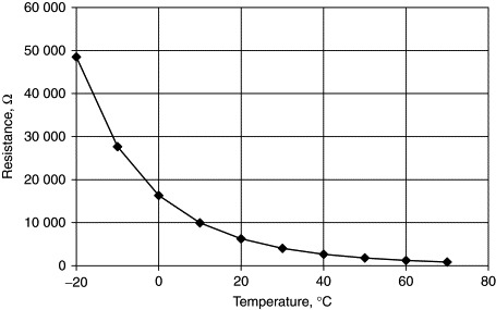
NTC thermistors exhibit many desirable features for temperature measurement and control. Their electrical resistance decreases with increasing temperature (see Figure 7.18) and the resistance–temperature relationship is very nonlinear. Depending upon the type of material used and the method of fabrication, thermistors can be used within the temperature range of −50° C to +150° C. The resistance of a thermistor is referenced to 25° C and for most applications the resistance at this temperature is between 100Ω and 100 kΩ.
Figure 7.18. Typical thermistor R/T characteristics.
The advantages of NTC thermistors are summarized next:
- Sensitivity One of the advantages of thermistors compared with thermocouples and RTDs is their relatively large change in resistance with temperature, typically −5% per degree Celsius.
- Small size Thermistors have very small sizes and this makes for a very rapid response to temperature changes. This feature is very important in temperature feedback control systems where a fast response is required.
- Ruggedness Most thermistors are rugged and can handle mechanical and thermal shock and vibration better than other types of temperature sensors.
- Remote measurement Thermistors can be used to sense the temperature of remote locations via long cables because the resistance of a long cable is insignificant compared to the relatively high resistance of a thermistor.
- Low cost Thermistors cost less than most of the other types of temperature sensors.
- Interchangeability Thermistors can be manufactured with very close tolerances. As a result of this it is possible to interchange thermistors without having to recalibrate the measurement system.
7.7.3. Self-Heating
A thermistor can experience self-heating as a result of the current passing through it. When a thermistor self-heats, the resistance reading becomes less than that of its true value and this causes errors in the measured temperature. The amount of self-heating is directly proportional to the power dissipated by the thermistor. In general, the larger the size of the thermistor and the higher the resistance, the more power it can dissipate. Also, a thermistor can dissipate more power in a liquid than in still air. The heat developed during operation will also be dissipated through the lead wires and it is important to make sure that the thermistor is mounted such that the contact areas do not get very hot.
The self-heating of a thermistor is measured by its dissipation constant (denoted by dth), which is generally expressed in mW/° C. There are different values depending upon whether or not the thermistor is used in still air or in a liquid. Typically, the dissipation constant is around 1 mW/° C in still air and around 8 mW/° C in stirred oil. For example, if the uncertainty in measurement due to self-heat is required to be 0.05° C, the maximum amount of power the thermistor is allowed to dissipate is 0.05° C × 1 mW/° C or 50 μW in still air and 400 μW in stirred oil. Knowing the resistance of the thermistor, we can calculate the maximum allowable current through the thermistor. Equation (7.18) shows the relationship between the dissipation constant and the thermal error due to self-heat of a thermistor: (7.18)
![]() where P is the power dissipated in the thermistor, Te is the thermal error due to self-heat, and dth is the dissipation constant of the thermistor.
where P is the power dissipated in the thermistor, Te is the thermal error due to self-heat, and dth is the dissipation constant of the thermistor.
Example 7.5
A thermistor is to be used as a sensor to measure the ambient temperature in a room. It is quoted that the dissipation constant in still air is 2 mW/° C. If the power dissipated by the thermistor is 200 μW, calculate the thermal error due to self-heat of the thermistor.
Solution 7.5
The thermal error can be calculated by using Equation (7.18).
![]() or
or
![]() or
or
![]()
7.7.4. Thermal Time Constant
Thermal time constant of a thermistor is the time required for a thermistor to reach 63.2% of a new temperature. Thermal time constant depends upon the type and mass of the thermistor and the method used for thermal coupling to its environment. A typical epoxy-coated thermistor has a thermal time constant of 0.7 s in stirred oil and 10 s in still air.
7.7.5. Thermistor Temperature–Resistance Relationship
Thermistor manufacturers usually provide the resistance–temperature characteristics of their devices either in the form of a table, a graph, or they provide some parameters that can be used to describe the behavior of a thermistor. All different techniques are described in this section.
7.7.5.1. Temperature–Resistance Table
Some manufacturers provide tables that give the resistance of their devices at different temperatures. Table 7.10 is an example temperature–resistance table where the temperature is specified in increments of 10° C and the resistance at any temperature can be estimated by interpolation. Some manufacturers provide tables with temperature increments of only 1° C or even lower.
Table 7.10. Typical thermistor temperature–resistance table
| Temperature (° C) | Resistance (ft) |
|---|---|
| −30 | 88,500 |
| −20 | 48,535 |
| −10 | 27,665 |
| 0 | 16,325 |
| +10 | 9,950 |
| +20 | 6,245 |
| +30 | 4,028 |
| +40 | 2,663 |
| +50 | 1,801 |
| +60 | 1,244 |
| +70 | 876 |
| +80 | 627 |
| +90 | 457 |
| +100 | 339 |
7.7.5.2. Steinhart-Hart fduation
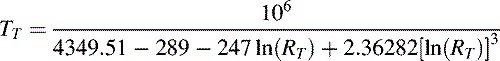
The Steinhart-Hart fduation is an empirically developed polynomial that best represents the temperature–resistance relationships of NTC thermistors. The Steinhart-Hart fduation is very accurate over the operating temperature of thermistors and it introduces errors of less than 0.1° C over a temperature range of −30° C to +125° C. To solve for temperature when resistance is known, the form of this fduation is (7.20)
![]() where TT is the measured temperature (K), RT is the resistance of the thermistor at temperature TT, and a, b, and c are thermistor coefficients.
where TT is the measured temperature (K), RT is the resistance of the thermistor at temperature TT, and a, b, and c are thermistor coefficients.
Equation (7.20) is usually written in the form (7.21)

The coefficients a, b, and c are sometimes given by the manufacturers. If these coefficients are not known, they can be calculated if the resistance is known at three different temperatures.
Using Equation (7.21), and assuming that the resistances of the thermistor at temperatures T1, T2, and T3 are R1, R2, and R3, respectively, we can write (7.22)
![]() (7.23)
(7.23)
![]() (7.24)
(7.24)
![]()
Equations (7.22), (7.23), and (7.24) are three fduations with three unknowns and these fduations can be solved to find the thermistor coefficients a, b, and c.
The resistances at three different temperatures can either be measured or they can be obtained from the temperature–resistance tables as in Table 7.10. An example follows to illustrate the method used.
Example 7.6
The temperature–resistance table of a thermistor is given in Table 7.10. Calculate the a, b, and c parameters of this thermistor and write down the Steinhart-Hart fduation.
Solution 7.6
We can write three equations with three unknowns by taking three points on the resistance–temperature curve.
Using Table 7.10 and taking three different temperatures,
![]()
![]()
![]() now, using Equations (7.22), (7.23), and (7.24) we can write (7.25)
now, using Equations (7.22), (7.23), and (7.24) we can write (7.25)
![]() (7.26)
(7.26)
![]() (7.27)
(7.27)
![]() or (7.28)
or (7.28)
![]() (7.29)
(7.29)
![]() (7.30)
(7.30)
![]()
Solving Equations (7.28), (7.29), and (7.30), the coefficients are
![]()
![]()
![]()
The Steinhart-Hart fduation can now be written as (7.31)
7.7.5.3. Using Temperature–Resistance Characteristic Formula
Some thermistor manufacturers give the resistances of their devices at 25° C and they also provide a thermistor temperature constant denoted by β. Equation (7.32) can be used to calculate the resistance at any other temperature: (7.32)
![]() where R25 is the resistance at 25° C, T25 is the temperature (in K) at 25° C, and β is the temperature constant of the thermistor.
where R25 is the resistance at 25° C, T25 is the temperature (in K) at 25° C, and β is the temperature constant of the thermistor.
The temperature can be calculated using Equation (7.32) as follows: (7.33)
 or (7.34)

An example follows to clarify the method used.
Example 7.7
The temperature constant of a thermistor is β = 2910. Also, the resistance of the thermistor at 25° C is R2 = 1 kΩ. This thermistor is used in an electrical circuit to measure the temperature and it is found that the resistance of the thermistor is 800Ω. Calculate the temperature.
Solution 7.7
First of all, the temperature at 25° C is converted into kelvins:
![]()
We can now use Equation (7.34).
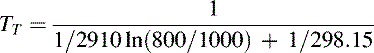 or
or
![]() or
or
![]()
The β Value
The temperature constant β depends upon the material used in manufacturing the thermistor. This parameter also depends on temperature and manufacturing tolerances, and as a result of this, Equation (7.34) is only suitable for describing a restricted range around the rated temperature or resistance with sufficient accuracy. The β values for common NTC thermistors range from 2000k through 5000k. For practical applications, the more complicated Steinhart-Hart fduation is more accurate.
Some manufacturers do not provide the value of β but they give the thermistor resistances at 25° C and also at 100° C. We can then calculate the value of β using Equation (7.32): (7.36)
 or (7.37)
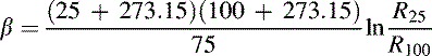 giving (7.38)
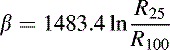
Thus, knowing the resistances at 25° C and also at 100° C we can use Equation (7.38) to calculate the value of β.
Example 7.8
The manufacturer of a certain type of thermistor specifies the resisce of the device at 25° C and at 100° C as 1000Ω and 600Ω, respectively. Calculate the temperature constant β of this thermistor.
Solution 7.8
The temperature constant β can be calculated using Equation (7.38).
![]() or
or
![]()
7.7.5.4. Thermistor Linearization
Thermistor sensors are highly nonlinear devices. It is possible to obtain very linear response from thermistors by connecting a resistor in parallel with the thermistor. The resistor value should be fdual to the thermistor's resistance at the mid range temperature of interest. The combination of a thermistor and a parallel resistor has an S-shaped temperature–resistance curve with a turning point.
7.7.6. Practical Thermistor Circuits
In this section we shall be looking at various techniques of using NTC thermistors to measure temperature. Because of the very high temperature constant of the thermistor, accurate temperature measurements can be made with very simple electrical circuits. Typical applications include temperature control of ovens, freezers, rooms, temperature alarms, chemical process control, and so on.
7.7.6.1. Constant Current Circuit
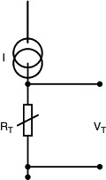
Figure 7.19 shows how a thermistor can be used in a very simple electrical circuit to measure temperature. A constant current I is passed through the thermistor which produces a voltage VT proportional to the current. By measuring this voltage and knowing the current, we can calculate the resistance of the thermistor as RT = VT/I and hence the temperature can be calculated by using Equations (7.20) or (7.32).
Figure 7.19. Constant current thermistor circuit.

7.7.6.2. Constant Voltage Circuit
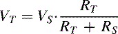
Figure 7.20 shows another simple thermistor circuit where a potential divider circuit is formed using a constant voltage source VS. The voltage VT across the thermistor is calculated as (7.39)
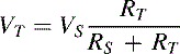
Figure 7.20. Constant voltage thermistor circuit.

Using Equation (7.39), the resistance of the thermistor can be found to be (7.40)
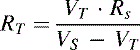
Once the resistance is found, we can use either Equation (7.20) or Equation (7.32) to calculate the temperature.
7.7.6.3. Bridge Circuit
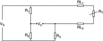
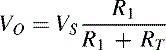
Figure 7.21 shows how the temperature can be measured using a simple electrical bridge circuit. Bridge circuits have the advantage that under balance conditions the resistance of the arms are independent of the supply voltage. In this circuit, the thermistor is in one of the arms of the bridge and resistor RV is used to balance the bridge. In the balance condition, the relationship between the resistors is (7.41)
 and the thermistor resistance can be found as (7.42)
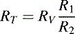
Figure 7.21. Thermistor bridge circuit.

The values of resistors R1, R2, and RV are all known and the temperature can be calculated by using RT in either Equation (7.20) or Equation (7.32).
In some applications it may not be practical to balance the bridge circuit. The value of RT can then be calculated as follows.
Let RV be a constant resistor such that RV = R2. When the bridge is not balanced, the value of VO is (7.43)
 and the thermistor resistance is (7.44)
7.7.6.4. Noninverting Operational Amplifier Circuit
Figure 7.22 shows how the thermistor can be used in a simple noninverting operational amplifier circuit to measure temperature. In this circuit, the output voltage VO is found as (7.45)
 where VS is the stabilized supply voltage. The thermistor resistance can be found as (7.46)

Figure 7.22. Noninverting operational amplifier thermistor circuit.

After finding RT, we can use Equation (7.20) or Equation (7.32) to calculate the temperature.
7.7.6.5. Inverting Operational Amplifier Circuit
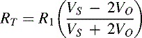
Figure 7.23 shows how a thermistor can be connected in the feedback path of an inverting operational amplifier. In this circuit, the output voltage VO is (7.47)
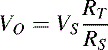
Figure 7.23. Inverting operational amplifier thermistor circuit.
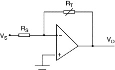
The thermistor resistance can be found as (7.48)
7.7.7. Microcontroller-Based Temperature Measurement
Thermistors give analog output voltages and the temperature can simply be displayed using an analog meter (e.g., a voltmeter). Although this may be acceptable for some applications, accurate temperature measurement and display require digital techniques.
Figure 7.24 shows how the temperature can be measured using a microcontroller. The temperature is sensed by the thermistor and a voltage is produced that is proportional to the measured temperature. This voltage is filtered using a low-pass filter to remove any unwanted high-frequency noise. The output of the filter is converted into digital form using a suitable A/D converter. The digitized voltage is then read by the microcontroller and the resistance of the thermistor is calculated. After this, the measured temperature can be calculated either by using a temperature–resistance table, or either Equation (7.20) or Equation (7.32). Finally, the temperature is displayed on a suitable digital display (e.g., an LCD). Although this approach is very simple and flexible, limitations arise in practice at both low and high temperatures. As the thermistor temperature decreases, its resistance increases and also the voltage across it increases. Practically the low temperature limit is reached when the voltage exceeds the maximum input voltage of the A/D converter. Similarly, when the thermistor temperature increases, its resistance decreases, so does the voltage across the thermistor. Practically the high temperature limit is reached when the voltage is less than the voltage resolution of the A/D converter. By varying the value of the constant current source in Figure 7.19 or the fixed voltage source in Figure 7.20, the useful temperature range of a thermistor can be extended for a given A/D converter.
Figure 7.24. Microcontroller-based temperature measurement.
![]()
7.8. Integrated Circuit Temperature Sensors
Integrated circuit temperature sensors are semiconductor devices fabricated in a similar way to other semiconductor devices such as microcontrollers. There are no generic types like the thermocouples or RTDs but some popular devices are manufactured by more than one manufacturer.
Integrated circuit temperature sensors differ from other sensors in some fundamental ways:
- These sensors have relatively small physical sizes
- Their outputs are linear (e.g., 10 mV/° C)
- The temperature range is limited (e.g., −40° C to +150° C)
- The cost is relatively low
- These sensors can include advanced features such as thermostat functions, built-in A/D converters and so on
- Often these sensors do not have good thermal contacts with the outside world and as a result it is usually more difficult to use them other than in measuring the air temperature
- A power supply is required to operate these sensors
Integrated circuit semiconductor temperature sensors can be divided into the following categories:
- Analog temperature sensors
- Digital temperature sensors
Analog sensors are further divided into
- Voltage output temperature sensors
- Current output temperature sensors
Analog sensors can either be directly connected to measuring devices (such as voltmeters), or A/D converters can be used to digitize the outputs so that they can be used in computer based applications.
Digital temperature sensors usually provide I2C bus, SPI bus, or some other three-wire interface to the outside world.
7.8.1. Voltage Output Temperature Sensors
These sensors provide a voltage output signal that is proportional to the temperature measured. There are many types of voltage output sensors and Table 7.11 gives some popular sensors. LM35 is a three-pin device and it has two versions and they both provide a linear output voltage of 10 mV/° C. The temperature range of the CZ version is −20° C to +120° C while the DZ version only covers the range 0° C to +100°. The accuracy of LM35 is around ±1.5°.
Table 7.11. Popular voltage output temperature sensor
| Sensor | Manufacturer | Output | Maximum error | Temperature range |
|---|---|---|---|---|
| LM35 | National Semiconductors | 10 mV/° C | ±1° C | −20° C to +120° C |
| LM34 | National Semiconductors | 10 mV/°F | ±3°F | −20° C to +120° C |
| LM50 | National Semiconductors | 10 mV/° C 500 mV offset | ±3° | −40° C to +125° C |
| LM60 | National Semiconductors | 6.25 mV/° C 424 mV offset | ±3° C | −40° C to +125° C |
| S-8110 | Seiko Instruments | −8.5 mV/° C | ±2.5° C | −40° C to +100° C |
| TMP37 | Analog Devices | 20 mV/° C | ±3° C | +5° C to +100° C |
LM34 is similar to LM35, but its output is calibrated in degrees Fahrenheit as 10 mV/°F.
LM50 can measure negative temperatures without any external components. The LM50's output voltage has a 10-mV/° C slope and a 500-mV offset; that is, the output voltage VO is (7.49)
![]()
Thus, the output voltage is 500 mV at 0° C, 100 mV at −40°, and 1.5V at 100° C.
LM60 gives a linear output of 6.25 mV/° C and it can operate with a supply voltage as low as 2.7V. The temperature range of this sensor is −40° C to 125° C.
S-8110 has a negative temperature coefficient and it gives −8.5 mV/° C. This sensor can operate at very low currents (10 μA) and the temperature range is −40° C to +100° C.
Analog Devices TMP37 is a high sensitivity sensor with a linear output voltage of 20 mV/° C and an operating temperature range of +5° C to +100° C.
7.8.1.1. Applications of Voltage Output Temperature Sensors
The popular LM35DZ temperature sensor is taken as an example in this section. As shown in Figure 7.25, this is a three-pin sensor. The maximum supply voltage is +35V, but the sensor is normally operated at +5V. When operated at +5V, the supply current is around 80 μA. The typical accuracy is ±0.6° C at +25° C.
Figure 7.25. LM35DZ is a three-pin sensor.

Figure 7.26 shows how the LM35DZ can be used to measure the temperature. The device is simply connected to a 4-V to 20-V power supply and the output voltage is a direct indication of the temperature in 10 mV/° C. A simple voltmeter can be connected and calibrated to measure the temperature directly. Alternatively, an A/D converter can be used to digitize the output voltage so that the sensor can be used in computer-based applications.
Figure 7.26. Using the LM35DZ to measure temperature.

Care should be taken when driving capacitive loads, such as long cables. To remove the effect of such loads, the circuit shown in Figure 7.27 should be used. Notice that a resistor is added to the output of the sensor, making this circuit suitable for connection to high impedance loads only.
Figure 7.27. Driving capacitive loads.

7.8.2. Current Output Temperature Sensors
Current output sensors act as high-impedance, constant-current sources, giving an output current that is proportional to the temperature. The devices operate typically between 4V and 30V and produce an output current of 1 μA/K. Table 7.12 gives a list of some popular current output sensors.
Table 7.12. Popular current output temperature sensors
| Sensor | Manufacturer | Output | Maximum error | Temperature range |
|---|---|---|---|---|
| AD590 | National Semiconductors | 1 μA/K | ±5.5° C | −55° C to +150° C |
| AD592 | Analog Devices | 1 μA/K | ±1° C | −25° C to +105° C |
| LM134 | Dallas Semiconductors | 0.1 μA/K to 4 μA/K | ±3° C | −25° C to +100° C |
AD590 has an operating temperature range of −55° C to +150° C and produces an output current of 1 μA/K.
AD592 is a more accurate sensor with a 1 μA/K and the temperature range is −25° C to 105° C. The maximum error within the operating range is ±1° C.
LM134 is a programmable sensor with an output current 0.1 μA/K to 4 μA/K. The sensitivity is set using a single external resistor. The temperature range of this sensor is −25° C to +100° C. LM134 typically needs only 1.2-V supply voltage, so it can be used in portable applications where the power is usually limited.
7.8.2.1. Applications of Current Output Temperature Sensors
The popular AD590 is taken as an example here. This device gives an output current that is directly proportional to the temperature; that is, (7.50)
![]() where I is in μA, T in kelvins, and k is the constant of proportionality (k = μA/K).
where I is in μA, T in kelvins, and k is the constant of proportionality (k = μA/K).
Figure 7.28 shows a typical application of the AD590. A constant voltage source is used to supply the circuit. The voltage across the resistor is measured and then the current is calculated. The temperature can then be calculated using Equation (7.50): (7.51)
![]()
Figure 7.28. Using AD590 to measure temperature.

![]()
![]() where T is in degrees Celsius, R is in ohms, and VR is in volts.
where T is in degrees Celsius, R is in ohms, and VR is in volts.
7.8.3. Digital Output Temperature Sensors
The digital output temperature sensors produce digital outputs that can be interfaced directly to computer-based fduipment. The outputs are usually nonstandard and the temperature can be extracted by using suitable algorithms. Table 7.13 gives a list of some popular digital output temperature sensors.
Table 7.13. Popular digital output temperature sensors
| Sensor | Manufacturer | Output | Maximum error | Temperature range |
|---|---|---|---|---|
| LM75 | National Semiconductors | I2C | ±3° C | −55° C to +125° C |
| TMP03 | Analog Devices | PWM | ±4° C | −25° C to +100° C |
| DS1620 | Dallas Semiconductors | 2 or 3 wire | ±0.5° C | −55° C to +125° C |
| AD7814 | Analog Devices | SPI | ±2° C | −55° C to +125° C |
| MAX6575 | Maxim | Single wire | ±0.8° C | −40° C to +125° C |
LM75 operates within the temperature range of −55° C to +125° C and provides an I2C bus compatible 9-bit serial output (1 sign bit and 8 magnitude bits), resulting in 0.5° C resolution. The device can be programmed to monitor the temperature. It can also set an output pin high or low if the temperature exceeds a preprogrammed value. The temperature can be read by I2C bus-compatible computer fduipment. The I2C bus algorithm can also be developed on microcontrollers. For example, the FED C compiler has built-in functions that support the I2C bus interface. LM75 has an addressable, multidrop connection feature which enables a number of similar sensors to be connected over the bus.
TMP03 provides PWM (pulse width modulation) output and the computer system it is connected to measures the width of the pulse to find the temperature. The temperature range is −25° C to +100° C.
DS1620 is a temperature sensor that also incorporates digitally programmable thermostat outputs. The device provides 9-bit temperature readings which indicate the temperature of the device. Temperature settings and temperature readings are all communicated to/from the DS1620 over a two- or three-wire interface.
AD7814 operates within the temperature range of −55° C to +125° C and provides SPI bus-compatible 10-bit resolution output. The temperature can be read by SPI bus-compatible computer equipment.
MAX6575 sensor enables multiplexing of up to eight sensors on a simple single-wire bidirectional bus. Temperature is sensed by measuring the time delays between the falling edge of an external triggering pulse and the falling edge of the subsequent pulse delays reported from the devices. Different sensors on the same line use different timeout multipliers to avoid overlapping signals. The temperature range of MAX6575 is −40° C to +125° C.
7.8.3.1. Applications of Digital Output Temperature Sensors
The popular DS1620 temperature sensor is considered in this section. Figure 7.29 shows the sensor pin configuration. DS1620 is a digital thermometer and thermostat IC that provides 9-bits of serial data to indicate the temperature of the device. VDD is the power supply which is normally connected to a +5-V supply. DQ is the data input/output pin. CLK is the clock input. RST is the reset input. The device can also act as a thermostat. THIGH is driven logic high if the DS1620's temperature is greater than or fdual to a user defined temperature TH. Similarly, TLOW is driven logic high if the DS1620's temperature is less than or fdual to a user defined temperature TL. TCOM is driven high when the temperature exceeds TH and stays high until the temperature falls below TL. User-defined temperatures TL and TH are stored in a nonvolatile memory of the device so that they are not lost even after removal of power.
Figure 7.29. Pin configuration of DS1620.

Data is output from the device as 9-bits, with the LSB sent out first. The temperature is provided in twos complement format from −55° C to +125° C, in steps of 0.5° C. Table 7.14 shows the relationship between the temperature and data output by the device.
Table 7.14. Temperature/data relationship of DS1620
| Temp. (° C) | Digital output (binary) | Digital output (hex) | Twos complement | Digital output (decimal) |
|---|---|---|---|---|
| +125 | 0 11111010 | 0FA | — | 250 |
| +25 | 0 00110010 | 032 | — | 50 |
| 0.5 | 0 00000001 | 001 | — | 1 |
| 0 | 0 00000000 | 000 | — | 0 |
| −0.5 | 1 11111111 | 1FF | 001 | 511 |
| −25 | 1 11001110 | 1CE | 032 | 462 |
| −55 | 1 10010010 | 192 | 06E | 402 |
Data input and output is through the DQ pin. When the RST input is high, serial data can be written or read by pulsing the clock input. Data is written or read from the device in two parts. First, a protocol is sent and then the required data is read or written. The protocol is 8-bit data and the protocol definitions are given in Table 7.15. For example, to write the thermostat value TH, the hexadecimal protocol data 01 is first sent to the device. After issuing this command, the next nine clock pulses clock in the 9-bit temperature limit which will set the threshold for operation of the THIGH output.
Table 7.15. DS1620 Protocol definitions
| Protocol | Protocol data (hex) |
|---|---|
| Write TH | 01 |
| Write TL | 02 |
| Write configuration | 0C |
| Stop conversion | 22 |
| Read TH | A1 |
| Read TL | A2 |
| Read temperature | AA |
| Read configuration | AC |
| Start conversion | EE |
For example, the following data (in hexadecimal) should be sent to the device to set it for a TH limit of +50° C and TL limit of +20° C and then subsequently to start conversion:
- 01 Send TH protocol
- 64 Send TH limit 50 (64 hex ·100 decimal)
- 02 Send TL protocol
- 28 Send TL limit of 20 (28 hex ·40 decimal)
- EE Send conversion start protocol
A configuration/status register is used to program various operating modes of the device. This register is written with protocol 0C (hex) and the status is read with protocol AC (hex). Some of the important configuration/status register bits are as follows:
- Bit 0 This is the 1 shot mode. If this bit is set, DS1620 will perform one temperature conversion when the start protocol is sent. If this bit is 0, the device will perform continuous temperature conversions.
- Bit 1 This bit should be set to 1 for operation with a microcontroller or microprocessor.
- Bit 5 This is the TLF flag and is set to 1 when the temperature is less than or fdual to TL.
- Bit 6 This is the THF flag and is set to 1 when the temperature is greater then or fdual to TH.
- Bit 7 This is the DONE bit and is set to 1 when a conversion is complete.