
Chapter 22. Measuring RF Emissions
One of the aspects of electromagnetic compatibility that is most difficult to grasp is the raft of techniques that are involved in making measurements. EMC phenomena extend in frequency to well beyond 1 GHz and this makes conventional and well-known techniques, established for low-frequency and digital work, quite irrelevant. Development and test engineers must appreciate the basics of high-frequency measurements in order to perform, or at least understand, the EMC testing that will be demanded of them. This chapter and the next will serve as an introduction to the equipment, the test methods and some of the causes of error and uncertainty that attend high-frequency EMC testing.
For ease of measurement and analysis, in the commercial tests radiated emissions are assumed to predominate above 30 MHz and conducted emissions are assumed to predominate below 30 MHz. There is of course no magic changeover at 30 MHz. But typical cable lengths tend to resonate above 30 MHz, leading to anomalous conducted measurements, while measurements of radiated fields below 30 MHz will of necessity be made in the near field if closer to the source than λ/2π, which gives results that do not necessarily correlate with real situations. In practice, investigations of interference problems have found that controlling the noise voltages developed at the mains terminals has been successful in alleviating radio interference in the long, medium and short wave bands (Jackson, 1989). At higher frequencies, mains wiring becomes less efficient as a propagation medium, and the dominant propagation mode becomes radiation from the equipment or wiring in its immediate vicinity. If you are considering military, aerospace, or automotive tests, the supply wiring is relatively less important as a principal route, and both conducted and radiated emissions tests are performed over a wider and overlapping frequency range.
Emissions testing requires that the equipment under test (EUT) is set up within a controlled electromagnetic environment under its normal operating conditions. If the object is to test the EUT alone, rather than as part of a system, its ancillary support equipment (if any) must be separately screened from the measurement (see Section 24.2.4.4). Any ambient signals should be well below the levels to which the equipment will be tested.
22.1. Emissions Measuring Instruments
22.1.1. Measuring Receiver
Conformance test measurements are normally taken with a measuring receiver, which is optimized for the purpose of taking EMC measurements. Typical costs for a complete receiver system to cover the range 10 kHz to 1 GHz can be anywhere between £15,000–£60,000.
Early measuring receivers were manually tuned and the operator had to take readings from the meter display at each frequency that was near the limit line. This was a lengthy procedure and prone to error. The current generation of receivers are fully automated and can be software controlled via an IEEE-488 standard bus; this allows a PC-resident program to take measurements with the correct parameters over the full frequency range of the test, in the minimum time consistent with gap-free coverage. Results are stored in the PC's memory and can be processed or plotted at will.
The distinguishing features of a measuring receiver compared to a spectrum analyzer are
- The receiver output is provided at a spot frequency, although high-end units can also provide a spectrum display
- Very much better sensitivity, allowing signals to be discriminated from the noise at levels much lower than the emission limits
- Robustness of the input circuits and resistance to overloading
- Intended specifically for measuring to CISPR standards, with bandwidths, detectors, and signal circuit dynamic range tailored for this purpose
- Frequency and amplitude accuracy is better than the cheaper spectrum analyzers
- Two units may be required, one covering up to 30 MHz and the other covering 30–1000 MHz or higher
22.1.2. Spectrum Analyzer
A fairly basic spectrum analyzer can be cheaper than a measuring receiver (typically £7,000–£15,000) and is widely used for “quick-look” testing and diagnostics. The instantaneous spectrum display is extremely valuable for confirming the frequencies and nature of offending emissions, as is the ability to narrow-in on a small part of the spectrum. When combined with a tracking generator, a spectrum analyzer is useful for checking the HF response of circuit networks.
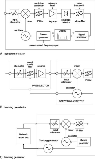
Basic spectrum analyzers are not an alternative to a measuring receiver in a full-compliance setup because of their limited sensitivity and dynamic range and susceptibility to overload. Figure 22.1(A) shows the block diagram of a typical spectrum analyzer. The input signal is fed straight into a mixer that covers the entire frequency range of the analyzer with no advance selectivity or preamplification. The consequences of this are threefold: First, the noise figure is not very good, so that when the attenuation due to the transducer and cable is taken into account, the sensitivity is hardly enough to discriminate signals from noise at the lower emission limits (see Section 22.2.1.1 later). Second, the mixer diode is a very fragile component and is easily damaged by momentary transient signals or continuous overloads at the input. If you take no precautions to protect the input, you will find your repair bills escalating quickly. Third, the energy contained in broadband signals can overload the mixer and drive it into nonlinearity even though the energy within the detector bandwidth is within the instrument's apparent dynamic range; this means you could be making an artificially low measurement, due to overloading, without realizing it.
Figure 22.1. Block diagram of spectrum analyzer.
22.1.2.1. Preselector
You can find instruments that offer a performance equivalent to that of a measuring receiver, but the price then becomes roughly equivalent as well. A more satisfactory compromise is to enhance the spectrum analyzer's front-end performance with a tracking preselector. The preselector (Figure 22.1(B)) is a separate unit that contains input protection, preamplification, and a swept tuned filter that is locked to the spectrum analyzer's local oscillator. The preamplifier improves the system noise performance to that of a test receiver. Equally important, the input protection allows the instrument to be used safely in the presence of gross overloads, and the filter reduces the energy content of broadband signals that the mixer sees, which improves the effective dynamic range.
The negative side of a preselector is that it can cost virtually as much as the spectrum analyzer itself, doubling the cost of the system. There are manual preselectors available, but these are clumsy to use. But you can treat it as an upgrade. The analyzer can be used on its own for diagnostics testing, and you can add a preselector when the time comes to make compliance measurements. Like the measuring receiver, modern spectrum analyzers and preselectors can be software controlled via an IEEE-488 bus, and provided the system hardware is adequate you can perform the compliance testing in exactly the same way (using a PC for the data processing).
22.1.2.2. Tracking generator
Including a tracking generator with the spectrum analyzer greatly expands its measuring capability without greatly expanding its price. With it, you can make many frequency-sensitive measurements that are a necessary feature of a full EMC test facility.
The tracking generator (Figure 22.1(C)) is a signal generator whose output frequency is locked to the analyzer's measurement frequency and is swept at the same rate. The output amplitude of the generator is maintained constant within very close limits, typically less than ±1 dB over 100 kHz to 1 GHz. If it provides the input to a network whose output is connected to the analyzer's input, the frequency/amplitude response of the network is instantly seen on the analyzer. While it is not as capable as a proper vector network analyzer, it gives some of the same functions at a fraction of the cost. The dynamic range could be theoretically equal to that of the analyzer (up to 120 dB), but in practice it is limited by stray coupling which causes feedthrough in the test jig.
You can use the tracking generator/spectrum analyzer combination for several tests related to EMC measurements:
- Characterize the loss of RF cables. Cable attenuation versus frequency must be accounted for in an overall emissions measurement.
- Perform open site attenuation calibration. The site loss between two calibrated antennas versus frequency is an essential parameter for open area test sites.
- Characterize components, filters, attenuators, and amplifiers. This is a vital tool for effective EMC remedies.
- Make tests of shielding effectiveness of cabinets or enclosures.
- Determine structural and circuit resonances.
22.1.3. Receiver Specifications
Whether you use a measuring receiver or spectrum analyzer, there are certain requirements laid down in the relevant standards for its performance. The “relevant standards” are CISPR 16-1-1 for CISPR-related tests and MIL STD 461E or DEF STAN 59-41 for military tests.
22.1.3.1. Bandwidth
The actual value of an interference signal that is measured at a given frequency depends on the bandwidth of the receiver and its detector response. These parameters are rigorously defined in a separate standard that is referenced by all the commercial emissions standards that are based on the work of CISPR, notably EN 55011, 55013, 55014-1, and 55022. This standard is CISPR publication 16-1-1 (CISPR, n.d.).
CISPR 16-1-1 splits the measurement range of 9 kHz to 1000 MHz into four bands and defines a measurement bandwidth for quasi-peak detection which is constant over each of these bands (Table 22.1). Sources of emissions can be classified into narrowband, usually due to oscillator and signal harmonics, and broadband, due to discontinuous switching operations, commutator motors, and digital data transfer. The actual distinction between narrowband and broadband is based on the bandwidth occupied by the signal compared with the bandwidth of the measuring instrument. A broadband signal is one whose occupied bandwidth exceeds that of the measuring instrument. Thus, a signal with a bandwidth of 30 kHz at 20 MHz (CISPR band B) would be classed as broadband, while the same signal at 40 MHz (band C) would be classed as narrowband.
Table 22.1. The CISPR 16-1 quasi-peak detector and bandwidths
| Quasi-peak detector | Frequency band | |||
|---|---|---|---|---|
| A, 9–150 kHz | B, 0.15–30 MHz | C, 30–300 MHz | D, 300–1000 MHz | |
| 6-dB bandwidth | 200 Hz | 9 kHz | 120 kHz | |
| Charge time constant, ms | 45 | 1 | 1 | |
| Discharge time constant, ms | 200 | 160 | 550 | |
| Predetector overload factor, dB | 25 | 30 | 43.5 |
Noise Level versus Bandwidth
The indicated level of a broadband signal changes with the measuring bandwidth. As the measuring bandwidth increases, more of the signal is included within it and hence the indicated level rises. The indicated level of a narrowband signal is not affected by measuring bandwidth. Noise, of course, is inherently broadband, and therefore there is a direct correlation between the “noise floor” of a receiver or spectrum analyzer and its measuring bandwidth: minimum noise (maximum sensitivity) is obtained with the narrowest bandwidth. The relationship between noise and bandwidth is given by Equation (22.1): (22.1)
![]()
For instance, a change in bandwidth from 10 kHz to 120 kHz would increase the noise floor by 10.8 dB.
22.1.3.2. Detector Function
There are three kinds of detector in common use in RF emissions measurements: peak, quasi-peak, and average. The characteristics are defined in CISPR 16-1-1 and are different for the different frequency bands.
Interference emissions are rarely continuous at a fixed level. A carrier signal may be amplitude modulated, and either a carrier or a broadband emission may be pulsed. The measured level that is indicated for different types of modulation will depend on the type of detector in use. Figure 22.2 shows the indicated levels for the three detectors with various signal modulations.
Figure 22.2. Indicated level versus modulation waveform for different detectors.

Peak
The peak detector responds near-instantaneously to the peak value of the signal and discharges fairly rapidly. If the receiver dwells on a single frequency the peak detector output will follow the “envelope” of the signal, hence it is sometimes called an envelope detector. Military specifications make considerable use of the peak detector, but CISPR emissions standards do not require it at all for frequencies below 1 GHz. However its fast response makes it very suitable for diagnostic or “quick-look” tests, and it can be used to speed up a proper compliance measurement.
Average
The average detector, as its name implies, measures the average value of the signal. For a continuous signal this will be the same as its peak value, but a pulsed or modulated signal will have an average level lower than the peak. The main CISPR standards call for an average detector measurement on conducted emissions, with limits which are 10–13 dB lower than the quasi-peak limits. The effect of this is to penalize continuous emissions with respect to pulsed interference, which registers a lower level on an average detector (Jennings and Kwan, 1986). A simple way to make an average measurement on a spectrum analyzer is to reduce the postdetector “video” bandwidth to well below the lowest expected modulation or pulse frequency (Linkwitz, 1991).
Quasi-Peak
The quasi-peak (QP) detector is a peak detector with weighted charge and discharge times (Table 22.1) which correct for the subjective human response to pulse-type interference. Interference at low pulse repetition frequencies (PRFs) is said to be subjectively less annoying on radio reception than that at high PRFs. Therefore, the quasi-peak response deemphasizes the peak response at low PRFs, or to put it another way, pulse-type emissions will be treated more leniently by a quasi-peak measurement than by a peak measurement. But to get an accurate result, the measurement must dwell on each frequency for substantially longer than the QP charge and discharge time constants.
Since CISPR-based tests have historically been intended to protect the voice and broadcast users of the radio spectrum, they lay considerable emphasis on the use of the QP detector. There is a point of view which suggests that with the advent of digital telecommunications and broadcasting this will change, since digital signals are affected by impulsive interference in a quite different way.
Possible Future Detectors
A study group within CISPR is looking at other means of detector weighting, and various documents have been circulated in the last few years. At the time of writing the favorite (CISPR, 2005) appears to be a weighting detector that is a combination of an rms detector (for pulse repetition frequencies above a corner frequency fc) and the average detector (for pulse repetition frequencies below the corner frequency fc), which achieves a pulse response curve with the following characteristics: 10 dB/decade above the corner frequency and 20 dB/decade below the corner frequency. The draft goes on to say: Nowadays the majority of disturbance sources may not contain repeated pulses, but still a great deal of equipment contains broadband emissions (with repeated pulses) and pulse modulated narrowband emissions. In addition, the transition from analog radiocommunication services to digital radiocommunication services has happened to a great deal and is partially still going on. The introduction of a new detector type may follow the transition from analog to digital radiocommunication systems. This transition may be regarded as a matter of frequency ranges: above 1 GHz, the use of digital radio communication systems is more frequent than below.
22.1.3.3. Overload Factor
A pulsed signal with a low duty cycle, measured with a quasi-peak or average detector, should show a level that is less than its peak level by a factor that depends on its duty cycle and the relative time constants of the quasi-peak detector and PRF. To obtain an accurate measurement the signal that is presented to the detector must be undistorted at very much higher levels than the output of the detector. The lower the PRF, the higher will be the peak value of the signal for a given output level (Figure 22.3). Conventionally, the input attenuator is set to optimize the signal levels through the receiver, but the required pulse response means that the RF and IF stages of the receiver must be prepared to be overloaded by up to 43.5 dB (for CISPR bands C and D) and remain linear. This is an extremely challenging design requirement and partially accounts for the high cost of proper measuring receivers and the unsuitability of spectrum analyzers for pulse measurements.
Figure 22.3. Relative output versus PRF for CISPR 16-1 detectors.
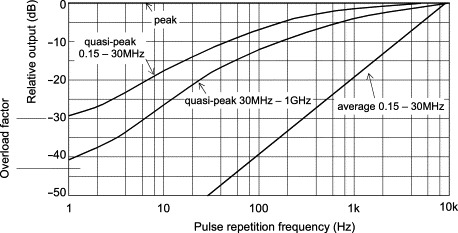
The same problem means that the acceptable range of PRFs that can be measured by an average detector is limited. The overload factor of receivers up to 30 MHz is only required to be 30 dB, and this degree of overload would be reached on an average detector with a pulsed signal having a PRF of less than 300 Hz. For this reason average detectors are only intended for measurement of continuous signals to allow for modulation or the presence of broadband noise and are not generally used to measure impulsive interference.
22.1.3.4. Measurement Time
Both the quasi-peak and the average detector require a relatively long time for their output to settle on each measurement frequency. This time depends on the time constants of each detector and is measured in hundreds of milliseconds. When a range of frequencies is being measured, the conventional method is to step the receiver at a step size of around half its measurement bandwidth, in order to cover the range fully without gaps (for the specified CISPR filter shape, the optimum step size is around 0.6 times the bandwidth, to give the largest step size consistent with maintaining the accuracy of measurement of any signal). For a complete measurement scan of the whole frequency range, as is required for a compliance test, the time taken is given by (22.2)
![]()
If the dwell time is restricted to three time constants, the time taken to do a complete quasi-peak sweep from 150 kHz to 30 MHz turns out to be 53 min. For an average measurement the scan time would be even longer, were it not for the way in which the average limit is applied. The difference between the quasi-peak and average limits is at most 13 dB (in CISPR 22, Class A) and this difference occurs at a PRF of 1.8 kHz. The decisive value for lower PRFs is always the QP indication. Therefore the average indication only has to be accurate for modulated or pulsed signals above this PRF, and this can be ensured with only a short dwell time, such as 1 ms.
But if you were to sweep with the quasi-peak detector, the dwell time would have to be increased to ensure that the peaks are captured and indicated correctly. It should be at least 1 s, if the signals to be measured are unknown. This has repercussions on the test method, as is discussed later in Chapter 23. It places correspondingly severe restrictions on the sweep rate when you are using a spectrum analyzer (Bronaugh, 1986).
22.1.3.5. Input VSWR
For any RF measuring instrument, the input impedance is crucial since amplitude accuracy depends on the maximum power transfer from the antenna, through the connecting cable to the receiver input. Invariably the system impedance is specified as 50Ω. As long as the receiver input is exactly 50Ω resistive, all the power is transferred without loss and hence without measurement error. Any departure from 50Ω causes some power to be reflected and there is said to be a “mismatch error.”
In practice the receiver input impedance cannot maintain a perfect 50Ω across the whole frequency range, and the degree to which it departs from this is called its VSWR (voltage standing wave ratio, see Section 23.5.2.1). VSWR can also be expressed differently as return loss or input reflection coefficient. A VSWR of 1:1 means no mismatch; CISPR 16-1-1 requires the receiver to have better than 2:1 VSWR with no input attenuation and better than 1.2:1 with 10 dB or greater input attenuation. There is a trade-off between input attenuation and sensitivity. As far as possible, receivers should be operated with at least 10 dB input attenuation since this gives a better match and greater accuracy, but this will bring the noise floor closer to the limit line, which may degrade accuracy. The EMC test engineer has to apply receiver settings that balance these two aspects and may require different settings at different frequencies. Both sources of error should be accounted for in the measurement uncertainty budget, as discussed in Section 23.5.
22.1.3.6. Other Measuring Instruments
Instruments have appeared on the market that fulfill some of the functions of a spectrum analyzer or receiver at a much lower price. These may be units that convert an oscilloscope into a spectrum display or that act as add-ons to a PC that performs the majority of the signal processing and display functions. Such devices are useful for diagnostic purposes provided that you recognize their limitations—typically frequency range, stability, bandwidth, and/or sensitivity. The major part of the cost of a spectrum analyzer or receiver is in its bandwidth-determining filters and its local oscillator. Cheap versions of these simply cannot give the performance that is needed of an accurate measuring instrument.
Even for diagnostic purposes, frequency stability and accuracy are necessary to make sense of spectrum measurements, and the frequency range must be adequate (150 kHz–30 MHz for conducted, 30 MHz–1 GHz for radiated diagnostics). Sensitivity matching that of a spectrum analyzer will be needed if you are working near to the emission limits. The inflexibility of the cheaper units soon becomes apparent when you want to make detailed tests of particular emission frequencies.
22.2. Transducers
For any RF emissions measurement you need a device to couple the measured variable into the input of the measuring instrumentation. Measured variables take one of four forms:
- Radiated electric field
- Radiated magnetic field
- Conducted cable voltage
- Conducted cable current
and the transducers for each of these forms are discussed next.
22.2.1. Antennas for Radiated Field
22.2.1.1. VHF-UHF Antennas
Radiated field measurements can be made of either electric (E) or magnetic (H) field components. In the far field the two are equivalent, and related by the impedance of free space: (22.3)
![]() but in the near field their relationship is complex and generally unknown. In either case, an antenna is needed to couple
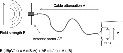
the field to the measuring receiver. Electric field strength limits are specified in terms of volts (or microvolts) per meter
at a given distance from the EUT, while measuring receivers are calibrated in volts (or microvolts) at the 50-Ω input. The antenna must therefore be calibrated
in terms of volts output into 50Ω for a given field strength at each frequency; this calibration is known as the antenna factor.
but in the near field their relationship is complex and generally unknown. In either case, an antenna is needed to couple
the field to the measuring receiver. Electric field strength limits are specified in terms of volts (or microvolts) per meter
at a given distance from the EUT, while measuring receivers are calibrated in volts (or microvolts) at the 50-Ω input. The antenna must therefore be calibrated
in terms of volts output into 50Ω for a given field strength at each frequency; this calibration is known as the antenna factor.
CISPR 16-1-4 defines transducers for radiated measurements. Historically its reference antenna has been a tuned dipole, but it also allows the use of broadband antennas, which remove the need for retuning at each frequency. Up until the mid-1990s the two most common broadband devices were the biconical, for the range 30–300 MHz, and the log periodic, for the range 300–1000 MHz. Some antennas have different frequency ranges.
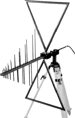
However, it is possible to combine a biconical and a log periodic to cover the range 30–1000 MHz or even wider. The two structures have been amalgamated with a means of ensuring that the feed is properly defined over the whole frequency range, and this type, originally designed at York University in the United Kingdom, is now available commercially. It is known, unsurprisingly, as the BiLog (Figure 22.4). Its major advantage, particularly appreciated by test houses, is that an entire radiated emissions (or immunity) test can be done without changing antennas, with a consequent improvement in speed and reliability. This has meant that the type is now almost universally used and versions are available from all the main EMC antenna manufacturers.
Figure 22.4. The BiLog (Schaffner).
The advantage of the tuned dipole is that its performance can be accurately predicted, but because it can only be applied at spot frequencies it is not used for everyday measurement but is reserved for calibration of broadband antennas, site surveys, site attenuation measurements, and other more specialized purposes.
Antenna Factor
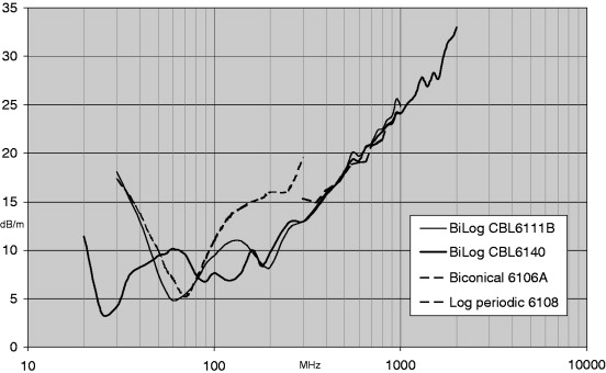
Those who use antennas for radio communication purposes are familiar with the specifications of gain and directional response, but these are of only marginal importance for EMC emission measurements. The antenna is always oriented for maximum response. Antenna factor is the most important parameter, and each calibrated broadband antenna is supplied with a table of its antenna factor (in decibels per meter, for E-field antennas) versus frequency. Antenna calibration is treated in more detail in Section 23.5.2.3. Typical antenna factors for a biconical, a log periodic, and two varieties of BiLog are shown in Figure 22.5. From this you can see that there is actually very little difference for the log periodic section (above 300 MHz) in particular: any LP design with the same dimensions will give substantially the same performance. The biconical (30–300 MHz) section can be “tweaked” but again, antennas with the same basic dimension give largely similar performance. This has the particular consequence that if all labs use pretty much the same design of antenna (which they do), the interlab variations in radiated field measurement due to the antenna itself are minimized.
Figure 22.5. Typical antenna factors (Schaffner).
To convert the measured voltage at the instrument terminals into the actual field strength at the antenna you have to add the antenna factor and cable attenuation (Figure 22.6). Cable attenuation is also a function of frequency; it can normally be regarded as constant with time, although long cables exposed to wide temperature variations, such as on open sites, may suffer slight variations of loss with temperature.
Figure 22.6. Converting field strength to measured voltage.
System Sensitivity
A serious problem can arise when using an antenna with a spectrum analyzer for radiated tests. Radiated emission compliance tests can be made at 10 m distance and the most severe limit in the usual commercial standards is the EN Class B level, which is 30 dBμV/m below 230 MHz and 37 dBμV/m above it. The minimum measurable level will be determined by the noise floor of the receiver or analyzer (see Section 22.1.3.1), which for an analyzer with 120-kHz bandwidth is typically +13 dBμV. To this must be added the antenna factor and cable attenuation in order to derive the overall measurement system sensitivity. Taking the antenna factors already presented, together with a typical 3 dB at 1 GHz due to cable attenuation, the overall system noise floor rises to 41 dBμV/m at 1 GHz as shown in Figure 22.7, which is 4 dB above the limit line.
Figure 22.7. System sensitivity.
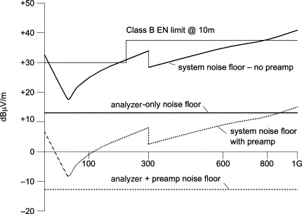
The CISPR 16-1-1 requirement on sensitivity is that the noise contribution should affect the accuracy of a compliant measurement by less than 1 dB. This implies a noise floor that is below the measured value by at least 6 dB.
Thus full radiated Class B compliance measurements cannot be made with a spectrum analyzer alone. Three options are possible: reduce the measuring distance to 3 m, which may raise the limit level by 10 dB, but this increases the measurement uncertainty and still gives hardly enough margin at the top end; or use a preamplifier or preselector to lower the effective system noise floor, by a factor equal to the preamp gain less its noise figure, typically 20–25 dB; or use a test receiver, which has a much better inherent sensitivity.
Polarization
In the far field the electric and magnetic fields are orthogonal. With respect to the physical environment, each field may be vertically or horizontally polarized, or in any direction in between. The actual polarization depends on the nature of the emitter and on the effect of reflections from other objects. An antenna will show a maximum response when its plane of polarization aligns with that of the incident field, and will show a minimum when the planes are at right angles. The plane of polarization of biconical, log periodic, and BiLog is in the plane of the elements. CISPR emission measurements must be made with “substantially plane-polarized” antennas; circularly polarized antennas, such as the log spiral, a broadband type once favored for military RF immunity testing, are outlawed.
22.2.1.2. The Loop Antenna
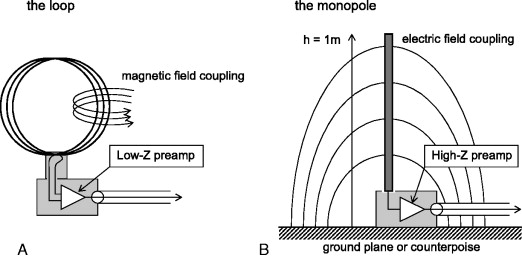
The majority of radiated emissions are measured in the range 30–1000 MHz. A few CISPR standards call for radiated measurements below 30 MHz. In these cases the magnetic field strength is measured using a loop antenna. Measurements of the magnetic field give better repeatability in the near-field region than do measurements of the electric field, which is easily perturbed by nearby objects. The loop (Figure 22.8(A)) is merely a coil of wire that produces a voltage at its terminals proportional to frequency, according to Faraday's law: (22.4)
![]() where N is the number of turns in the loop; A is the area of the loop, m2; F is the measurement frequency, Hz; H is the magnetic field, A/m.
where N is the number of turns in the loop; A is the area of the loop, m2; F is the measurement frequency, Hz; H is the magnetic field, A/m.
Figure 22.8. Low-frequency antennas.
The low impedance of the loop does not match the 50-Ω impedance of typical test instrumentation. Also, the frequency dependence of the loop output makes it difficult to measure across more than three decades of frequency, typically 9 kHz to 30 MHz. Passive loops deal with this latter problem by switching in different numbers of turns to cover smaller subranges in frequency, but naturally this does not lend itself to test automation.
These disadvantages are overcome by including as part of the antenna a preamplifier that corrects for the frequency response and matches the loop output to 50Ω. The preamp can be battery powered or powered from the test instrument. Such an “active” loop has a flat antenna factor across its frequency range. Its disadvantage by comparison with a passive loop is that it can be saturated by large signals, and some form of overload indication is needed to warn of this.
The Van Veen Loop
A disadvantage of the loop antenna as it stands is its lack of sensitivity at low frequencies. An alternative method (Bergervoet and van Veen, 1989) is to actually surround the EUT with the loop; in its practical realization, three orthogonal loops of 2–4-m diameter are used with the current induced in each being sensed by a current transformer, and the three signals are measured in turn by the test receiver. This is the large loop antenna (LLA) or Van Veen loop, named after its inventor, and it is specified in EN 55015, the standard for lighting equipment.
22.2.1.3. The Electric Monopole
The complementary antenna to the loop is the monopole (Figure 22.8(B)). Covering the frequency range again typically up to 30 MHz, the monople is simply a single vertical rod of length 1 m referenced against a ground plane or “counterpoise,” and it measures the electric field in vertical polarization. It is not used in many CISPR-based tests, only the automotive emissions standards CISPR 12 and CISPR 25 call it up, but it is used fairly widely in military testing to DEF STAN 59-41 and its American equivalent, MIL STD 461E. These tests require low frequency measurement of both the E-field and the H-field strengths.
The monopole is electrically short (its length is much less than a wavelength) and its source impedance looks like a capacitance of a few picofarads. So just as with the loop it is not suitable for connecting directly to a 50-Ω measuring system, and it should be fitted with a high impedance preamplifier to give impedance matching and to give a flat antenna factor. This makes it sensitive to damage and to electrical overload by large signals during the measurement—including the all-pervasive 50-Hz mains E-field—so again it needs an overload indicator and a high-pass filter to remove the mains field. Because the near electric field can be affected by the presence of virtually any conducting object, the accuracy and repeatability of measurements made with this antenna is poor even by the standards of EMC testing.
22.2.2. LISNs and Probes for Cable Measurements
22.2.2.1. Artificial Mains Network
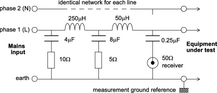
To make conducted voltage emissions tests on the mains port, you need an artificial mains network (AMN) or line-impedance stabilizing network (LISN) to provide a defined impedance at RF across the measuring point, to couple the measuring point to the test instrumentation, and to isolate the test circuit from unwanted interference signals on the supply mains. The most widespread type of LISN is defined in CISPR 16-1-2 and presents an impedance equivalent to 50Ω in parallel with 50 μH + 5Ω across each line to earth (Figure 22.9). This is termed a V network since for a single-phase supply the impedance appears across each arm of the V, where the base of the V is the reference earth.
Figure 22.9. LISN impedance versus frequency.

Note that its impedance is not defined above 30 MHz, partly because commercial mains conducted measurements are not required above this frequency (although military and automotive standards are) but also because component parasitic reactances make a predictable design difficult to achieve. An alternative 50-Ω/5-μH network is available in the CISPR specification, and a similar version is widely used in military and automotive tests according to DEF STAN 59-41 and MIL STD 461E. Since it uses a smaller inductor, it can carry higher currents and its impedance can be controlled up to 100 MHz and beyond. The military LISN's impedance is specified down to 1 kHz and up to 400 MHz. It is principally intended to simulate DC supplies but can also be used for mains tests when higher current ratings, typically above 50 A, are needed.
CISPR 16-1-2 includes a suggested circuit (Figure 22.10) for each line of the LISN, but it only actually defines the impedance characteristic. The main impedance determining components are the measuring instrumentation input impedance, the 50-μH inductor, and the 5-Ω resistor. The remaining components serve to decouple the incoming supply. The 5-Ω resistor is only effective at the bottom end of the frequency range, and in fact a “cut-down” version of LISN is defined that omits it and the 250-μH inductor but is restricted to frequencies above 150 kHz. Most commercial LISNs, though, include the whole circuit and cover the range down to 9 kHz. A common addition is a high-pass filter between the LISN output and the receiver, cutting off below 9 kHz, to prevent the receiver from being affected by high-level harmonics of the mains supply itself. Of course, this filter has to maintain the 50-Ω impedance and have a defined (preferably 0 dB) insertion loss at the measured frequencies.
Figure 22.10. LISN circuit per line.
An extension to the LISN specification is underway at the time of writing in the form of an amendment to CISPR 16-1-2 (CISPR, 2006). This tightens various aspects of the impedance requirement, in particular that it should have a phase angle tolerance of better than ±11.5° across the whole frequency range, even up to 30 MHz. This new requirement will be difficult to meet for some existing LISNs, particularly larger ones at the high-frequency end, because of stray capacitance. The justification for it is that, if you are going to calculate a complete measurement uncertainty budget for the conducted emissions test, a boundary needs to be placed on the possible range of impedance in both magnitude and phase presented by the LISN, otherwise the uncertainty due to impedance variations is unknown. It seems, though, debatable whether the greater complexity in calibration will be worthwhile when other, larger sources of uncertainty in what is already a reasonably well-specified test remain unaddressed (Section 23.5.2.2).
Current Rating
For the user, the most important parameter of the LISN is its current rating. Since the inductors are in series with the supply current, their construction determines how much current can be passed; if they are air cored, then magnetic saturation is not a problem but the coils may still overheat with too much current. Most LISNs use air cored coils, but if magnetic cores are used (typically iron powder) for a smaller construction then you also need to be concerned about saturation, which will affect the impedance characteristic of the device.
Another effect of the impedance of the inductors is the voltage drop that may appear between the supply feed and the EUT terminals. At 50 Hz the total in-line inductance of 600 μH gives an impedance of about 0.2Ω, which may itself give a significant voltage drop, added to the resistance through the unit, at high currents; but if, as may happen with an electronic power supply, your unit draws substantial harmonics of 50 Hz, then the inductive impedance of a few ohms at a few hundred hertz can give a much greater voltage drop with attendant waveform distortion. This in turn could affect the functional performance of the EUT.
Limiter
The spectrum analyzer's input mixer is a very fragile component. As well as being affected by high-level continuous input signals it is also susceptible to transients. Unfortunately the supply mains is a fruitful source of such transients, which can easily exceed 1 kV on occasion. These transients are attenuated to some extent by the LISN circuitry but it cannot guarantee to keep them all within safe limits. More important, switching operations within the EUT itself are likely to generate large transients due to interruption of current through the LISN chokes, and these are fed directly to the analyzer without attenuation.
For this reason it is essential to include a transient limiter in the signal cable between the LISN and the spectrum analyzer. This adds an extra 10-dB loss (typically) in the signal path which must be added to the LISN's own transducer factor, since the limiting devices need to be fed from a well-defined impedance, but this can normally be tolerated and is a much cheaper option than expensive repair bills for the analyzer front end. The limiter circuit generally uses a simple back-to-back diode clipping scheme; some limiters also incorporate a filter to restrict the frequency range transmitted to the analyzer.
A limiter is less necessary, though still advisable, when a measuring receiver is used since the receiver's front end should be already protected. The limiter does have one particular danger: Low-frequency signals that are outside the measurement range and therefore not subject to limits may legitimately have amplitudes of volts, which will drive the limiter into continuous clipping and create harmonics that are then incorrectly measured as in-band signals. If you suspect such an eventuality, be prepared to place extra attenuation or high-pass filtering before the limiter to check.
Earth Current
A large capacitance (in total around 12 μF) is specified between line and earth, which when exposed to the 230-V line voltage results in around 0.9A in the safety earth. This level of current is lethal, and the unit must therefore be solidly connected to earth for safety reasons. If it is not, the LISN case, the measurement signal lead and the equipment under test can all become live. As a precaution, you are advised to bolt your LISN to a permanent ground plane and not allow it to be carried around the lab! A secondary consequence of this high earth current is that LISNs cannot be used directly on mains circuits that are protected by earth leakage or residual current circuit breakers. Both of these problems can be overcome by feeding the mains to the LISN through an isolating transformer, provided that this is sized adequately, bearing in mind the extra voltage drop through the LISN itself.
Diagnostics with the LISN
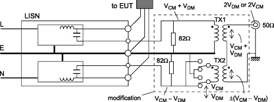
As it stands, the LISN does not distinguish between differential mode (line-to-line) and common mode (line-to-earth) emissions; it merely connects the measuring instrument between phase and earth. A modification to the LISN circuit (Figure 22.11) allows you to detect either the sum or the difference of the live and neutral voltages, which correspond to the common mode and differential mode voltages, respectively (Paul and Hardin, 1988). This is not required for compliance measurements but is very useful when making diagnostic tests on the mains port of a product. Transformers TX1 and 2, which can be nothing more than 50-Ω 1:1 broadband balun parts, are switched to add or subtract the two signals.
Figure 22.11. Modifying the LISN to measure differential or common mode.
22.2.2.2. Absorbing Clamp and CMAD
As well as measuring the emissions above 30 MHz directly as a radiated field, you can also measure the disturbances that are developed in common mode on connected cables. Standards that apply primarily to small apparatus connected only by a mains cable—notably EN 55014-1—specify the measurement of interference power present on the mains lead. This has the advantage of not needing a large open area for the tests, but it should be done inside a fairly large screened room and the method is somewhat clumsy. The transducer is an absorbing device known as a ferrite clamp.
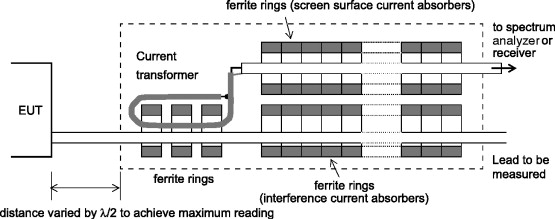
The ferrite absorbing clamp (often referred to as the MDS-21 clamp, and different from the EM-clamp used in immunity tests despite its similar appearance) consists of a current transformer using two or three ferrite rings, split to allow cable insertion, with a coupling loop (Figure 22.12). This is backed by further ferrite rings forming a power absorber and impedance stabilizer, which clamps around the mains cable to be measured. The device is calibrated in terms of output power versus input power, that is, insertion loss. The purpose of the ferrite absorbers is to attenuate reflections on the lead under test downstream of the current transformer; this is not 100% effective, and a full compliance test requires the clamp to be traversed for a half wavelength along the cable, that is, 5 m, to find a maximum. The lead from the current transformer to the measuring instrument is also sheathed with ferrite rings to attenuate screen currents on this cable. Because the output is proportional to current flowing in common mode on the measured cable, it can be used as a direct measure of noise power, and the clamp can be calibrated as a two-port network in terms of output power versus input power.
Figure 22.12. The ferrite absorbing clamp.
CISPR 16-1-3 specifies the construction, calibration, and use of the ferrite clamp. As well as its use in certain compliance tests, it also lends itself to diagnostics as it can be used for repeatable comparative measurements on a single cable to check the effect of circuit changes. It has been suggested (Stecher, 1995) that the clamp should be used to “pretest” small EUTs, with the application of a suitable empirically derived correction factor, so that they need only be subjected to a radiated test at the most critical emitting frequencies, but this idea has not been pursued within the standards.
The CMAD
A further common use for the clamp is to be applied to the further end of connected cables, both in radiated emissions and immunity tests, to damp the cable resonance and reduce variations due to cable termination. The clamp output is not connected when it is used in this way. Although this is a convenient method if a clamp is already to hand, using a string of 6–10 large snap-on ferrite sleeves is almost as effective. Alternatively, you can obtain commercially a unit known as a common-mode absorbing device (CMAD) which is the same thing. Amendment A1 to the third edition of CISPR 22 specified such a device to be applied to cables leaving the radiated emissions test site, whose purpose was simply to stabilize the far-end cable impedance and therefore make for a more repeatable test.
Despite this worthy aim, the amendment sparked such a howl of protest that it was abandoned and later editions of the standard make no reference to cable common-mode impedance stabilization. Many of the reasons against using CMADs in this way demonstrated a lack of understanding of the purpose of the amendment; for instance, it was claimed that such clamps would never be used in real installations and therefore the test would not be representative; but there is really no way that such test setups can ever be both truly representative and repeatable. The merit of the CMAD is that it would ensure a high impedance at a fixed distance from the EUT and therefore improve repeatability, and at the same time represent one installation condition where such an impedance did occur.
A more reasonable objection to the amendment was that, at the time, no method was published for verifying the impedance of the CMAD. This is now being addressed and a draft amendment to CISPR 16-1-4 is in progress. This author is wholeheartedly in favor of using some kind of CMAD to control the cable impedances in the radiated tests; even if the compliance test stubbornly refuses to address the issue, your precompliance measurements will be easier to repeat if you do.
22.2.2.3. Current Probe
Also useful for diagnostics is the current probe, which does the same thing as the absorbing clamp except that it does not have the absorbers. It is simply a clamp-on, calibrated wideband current transformer. Military specifications call for its use on individual cable looms, and the third edition of EN 55022 giving test methods for telecoms ports also requires a current probe for some versions of the tests. CISPR 16-1 includes a specification for the current probe. Because the current probe does not have an associated absorber, the RF common-mode termination impedance of the line under test should be defined by an impedance stabilizing network, which must be transparent to the signals being carried on the line.
Both the ferrite clamp and the current probe have the great advantage that no direct connection is needed to the cable under test, and disturbance to the circuit is minimal below 30 MHz since the probe effect is no more than a slight increase in common-mode impedance. But at higher frequencies the effect of the common-mode coupling capacitance between probe and cable becomes significant, as does the exact position of the probe along the cable, because of standing waves on the line. Your test plan and report should note this position exactly, along with the method of bonding the current probe case to the ground plane, which controls the stray capacitance.
22.2.2.4. ISNs and Other Methods for Telecom Port Conducted Emissions
The third edition of EN 55022 has provisions for tests on telecommunications ports. The preferred method uses a particular variant of impedance stabilizing network (ISN) which is designed to mimic the characteristics of balanced, unscreened ISO/IEC 11801 data cables. This network has a common mode impedance of 150Ω and a carefully controlled longitudinal conversion loss (LCL); that is, the parameter that determines the conversion from differential-mode signal to common-mode interference currents. Both current and voltage limits are published, related by the 150-Ω impedance.
The telecom port test has been controversial since the third edition was published. The basic problem is that, since it applies to ports such as local area network (LAN) interfaces, the signal that is intended to be passed through the port—data up to, say, 100 Mb/s—is in the same frequency range as the interference to be measured. The wanted signal is in differential mode while the interference is in common mode. Therefore, for a given data amplitude as determined by the network in use, such as Ethernet, the interference you measure is at least partly determined by the LCL of the network that is used for the measurement to represent a particular type of cable. There will be two components to the measurement:
- The wanted data converted from differential to common mode by the LCL
- Any extraneous common-mode noise added by imperfections in the design of the port
Of course, the second of these must be controlled, and so the test is necessary, but the first should not be allowed to spoil the measurement unnecessarily. Hence a need for a very careful specification of the LCL of the impedance stabilizing network, since all other parameters are invariant. The initial version of the standard paid insufficient attention both to this question and to the proper calibration of the ISN, and it took some time for the issue to be sorted out. The fifth edition of EN 55022 has apparently corrected the problems and its values of LCL are shown graphically in Figure 22.13, but in the meantime earlier versions were not acceptable for full compliance purposes in respect of the telecom port test, and for that reason their dates of mandatory implementation kept being postponed.
Figure 22.13. An example ISN circuit and the LCL specification.

As well as using ISNs with specified parameters for signal lines with balanced, unscreened pairs, the telecom port test is also applied to signal lines that use other kinds of cable. It is not always possible to specify an ISN for every one of these, and so alternative and preferably no-invasive methods of measurement have been and still are needed. These are described in Annex C of the standard and include
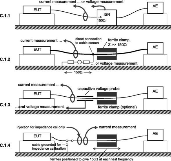
- Using alternative ISNs, such as the CDNs used for conducted immunity tests to IEC 61000-4-6, as long as the EUT can operate normally with this inserted, and as long as the CDN has a calibrated minimum LCL (C.1.1)
- For shielded cables, using a 150-Ω load to the outside surface of the shield in conjunction with a ferrite decoupler (C.1.2)
- Using a combination of current probe and capacitive voltage probe, and comparing the result to both current and voltage limits (C.1.3)
- Using a current probe only, but with the common mode impedance on the ancillary equipment side of the probe explicitly set to 150Ω at each test frequency with a ferrite decoupler (C.1.4)
The various methods are illustrated in Figure 22.14. In the fifth edition of EN 55022 improvements have been made over the original, although even so the method of C.1.4 is so cumbersome that the standard itself says, “If the method in C.1.4 is combined with the method of C.1.3, it is possible to use the advantages of both methods, without suffering too much from the disadvantages” and in fact it is wise to avoid it if at all possible. The EMC Test Laboratories Association (n.d.) published a Technical Guidance Note (TGN42) dealing with the various difficulties and questions raised by the test as originally published, in an attempt to help labs to arrive at a common interpretation of the methods.
Figure 22.14. Alternative telecom port measurement methods.
22.2.3. Near-Field Probes
Very often you will need to physically locate the source of emissions from a product. A set of near-field (or “sniffer”) probes is used for this purpose. These are so called because they detect field strength in the near field, and therefore two types of probe are needed, one for the electric field (rod construction) and the other for the magnetic field (loop construction). It is simple enough to construct adequate probes yourself using coax cable (Figure 22.15), or you can buy a calibrated set. A probe can be connected to a spectrum analyzer for a frequency domain display, or to an oscilloscope for a time domain display.
Figure 22.15. Do-it-yourself near-field probes.
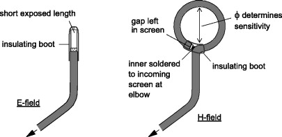
Probe design is a trade-off between sensitivity and spatial accuracy. The smaller the probe, the more accurately it can locate signals but the less sensitive it will be. You can increase sensitivity with a preamplifier if you are working with low-power circuits. A good magnetic field probe is insensitive to electric fields and vice versa; this means that an electric field probe will detect nodes of high dv/dt but will not detect current paths, while a magnetic field probe will detect paths of high di/dt but not voltage points.
Near-field probes can be calibrated in terms of output voltage versus field strength, but these figures should be used with care. Measurements cannot be directly extrapolated to the far-field strength (as on an open site) because in the near field one or other of the E or H fields will dominate depending on source type. The sum of radiating sources will differ between near and far fields, and the probe will itself distort the field it is measuring. Perhaps more important, you may mistake a particular “hot spot” that you have found on the circuit board for the actual radiating point, whereas the radiation is in fact coming from cables or other structures that are coupled to this point via an often complex path. Probes are best used for tracing and for comparative rather than absolute measurements.
22.2.3.1. Near-Field Scanning Devices
A particular implementation of a near-field probe is the planar scanning device, such as EMSCAN. This was developed and patented at Bell Northern Research in Canada and is now marketed by EmScan Corporation of Canada, as well as having competitors from other manufacturers. In principle it is essentially a planar array of tiny near-field current probes arranged in a grid form on a multilayer PCB (Ettles, 1990). The output of each current probe can be switched under software control to a frequency-selective measuring instrument, whose output in turn provides a graphical display on the controlling workstation. An alternative method uses a single probe positioned by X-Y stepper motors, in the same way as an X-Y plotter.
The device is used to provide a near-instantaneous two-dimensional picture of the RF circulating currents within a printed circuit card placed over the scanning unit. It can provide either a frequency versus amplitude plot of the near field at a given location on the board or an x-y coordinate map of the current distribution at a given frequency. For the designer it can quickly show the effect of remedial measures on the PCB being investigated, while for production quality assurance it can be used to evaluate batch samples which can be compared against a known good standard.
22.2.4. The GTEM for Emissions Tests
The GTEM for radiated RF immunity testing can also be used for emissions tests with some caveats. The GTEM is a special form of enclosed TEM (transverse electromagnetic mode) transmission line that is continuously tapered and terminated in a broadband RF load. This construction prevents resonances and gives it a flat frequency response from DC to well beyond 1 GHz. An EUT placed within the transmission line will couple closely with it, and its radiated emissions can be measured directly at the output of the cell. Since far-field conditions also describe a TEM wave, any test environment that provides TEM wave propagation should be acceptable as an alternative. The great advantages of this technique are that no antenna or test site is needed, the frequency range can be covered in a single sweep, and ambients are eliminated.
However, compliance tests demand a measure of the radiated emissions as they would be found on an OATS (see next section). This requires that the GTEM measurements are correlated to OATS results. This is done in software and the model was originally described in (Wilson, Hansen, and Koenigstein, 1989). In fact, three scans are done with the EUT in orthogonal orientations within the cell. The software then derives at each frequency an equivalent set of elemental electric and magnetic dipole moments, and then recalculates the far-field radiation at the appropriate test distance from these dipoles.
The limitation of this model is that the EUT must be “electrically small”; that is, its dimensions are small when compared to a wavelength. Connected cables pose a particular problem since these often form the major radiating structure and are of course rarely electrically small, even if the EUT itself is. Good correlation has been found experimentally for small EUTs without cables (Bronaugh and Osburn, 1991; Porter et al., 1994), but the correlation worsens as larger EUTs, or EUTs with connected cables, are investigated.
There is now a standard for measurements of both emissions and immunity in TEM cells, IEC 61000-4-20 (n.d.). This expands on the OATS correlation and gives a detailed description of the issues involved in using any kind of TEM cell, including the GTEM, for radiated tests, but its limitation is apparent in Clause 6:
- Small EUT An EUT is defined as a small EUT if the largest dimension of the case is smaller than one wavelength at the highest test frequency (for example, at 1 GHz λ = 300 mm), and if no cables are connected to the EUT. All other EUTs are defined as large EUTs.
- Large EUT An EUT is defined as a large EUT if it is
- A small EUT with one or more exit cables
- A small EUT with one or more connected nonexit cables
- An EUT with or without cable(s) which has a dimension larger than one wavelength at the highest test frequency
- A group of small EUTs arranged in a test setup with interconnecting nonexit cables, and with or without exit cables.
For emissions tests, it then goes on to state that “Large EUTs and specific considerations regarding EUT arrangements and cabling are deferred for elaboration in the next edition of this standard”; in other words virtually all real EUTs cannot be treated under the current version.
In practice the GTEM is a useful device for testing small EUTs without cables and can be applied in a number of specialized applications such as for measuring direct emissions from integrated circuits. But, although IEC 61000-4-20 has been published, it does not specify the tests to be applied to any particular apparatus or system. Instead it is meant to provide a general basic reference for all interested product committees, and its popularity will depend on it being referenced widely in conventional product emissions standards. The OATS correlation is limited in its full applicability to only a few types of EUT, and the likelihood that the GTEM will inhabit more than a restricted niche in EMC testing is small. Meanwhile, the National Physical Laboratory Electromagnetic Metrology Group has published a Best Practice Guide (Nothofer et al., 2005) for the GTEM which expands on the practicalities of IEC 61000-4-20 measurements. Anybody who uses a GTEM should have both of these documents as a reference.
22.3. Sites and Facilities
22.3.1. Radiated Emissions
22.3.1.1. The CISPR OATS
For CISPR-based standards, the reference for radiated emissions compliance testing is an open-area test site (OATS). The characteristics of a minimum standard OATS are defined in EN 55022 and CISPR 16-1-4 and some guidance for construction is given in ANSI C63.7 (ANSI, 1988). Such a site offers a controlled RF attenuation characteristic between the emitter and the measuring antenna (known as site attenuation). To avoid influencing the measurement there should be no objects that could reflect RF within the vicinity of the site. The original CISPR test site dimensions are shown in Figure 22.16.
Figure 22.16. The CISPR OATS.

The ellipse defines the area that must be flat and free of reflecting objects, including overhead wires. In practice, for good repeatability between different test sites, a substantially larger surrounding area free from reflecting objects is advisable. This means that the room containing the control and test instrumentation needs to be some distance away from the site. An alternative is to put this room directly below the ground plane, either by excavating an underground chamber (as long as your site's water table will allow it) or by using the flat roof of an existing building as the test site. Large coherent surfaces will be a problem, but not smaller pieces of metal for door hinges, door knobs, light fixtures at ground level, bolts, and metal fittings in primarily nonconductive furniture. Do not put your site right next to a car park!
Ground Plane
Because it is impossible to avoid ground reflections, these are regularized by the use of a ground plane. The minimum ground plane dimensions are also shown in Figure 22.16.
Again, an extension beyond these dimensions will bring site attenuation closer to the theoretical; scattering from the edges contributes significantly to the inaccuracies, although these can be minimized by terminating the edges into the surrounding soil (Maas and Hoolihan, 1989). Close attention to the construction of the ground plane is necessary. It should preferably be solid metal sheets welded together, but this may be impractical over the whole area. Bonded wire mesh is suitable, since it drains easily and resists warping in high temperatures if suitably tensioned. For RF purposes it must not have voids or gaps that are greater than 0.1λ at the highest frequency (i.e., 3 cm). Ordinary wire mesh is unsuitable unless each individual overlap of the wires is bonded. CISPR 16-1 suggests a ground plane surface roughness of better than 4.5 cm. The surface should not be covered with any kind of lossy dielectric—floor paint is acceptable but nothing much more than that.
Measuring Distance
The measurement distance d between EUT and receiving antenna determines the overall dimensions of the site and hence its expense. There are three commonly specified distances: 3 m, 10 m, and 30 m, although 30 m is rarely used in practice. In EN 55022 and related standards the measuring distance is defined between the boundary of the EUT and the reference point of the antenna. Although the limits are usually specified at 10-m distance, tests can be carried out on a 3-m range, on the assumption that levels measured at 10 m will be 10.5 dB lower (field strength should be proportional to 1/d). This assumption is not entirely valid at the lower end of the frequency range, where 3-m separation is approaching the near field, and indeed experience from several quarters shows that a linear 1/d relationship is more optimistic than is found in practice. Nevertheless because of the expense of the greater distance, especially in an enclosed chamber, 3-m measurements are widely used.
Weatherproofing
The main environmental factor that affects open area emissions testing, particularly in Northern European climates, is the weather. Some weatherproof but RF-transparent structure is needed to cover the EUT to allow testing to continue in bad weather. The structure can cover the EUT alone, for minimal cost, or can cover the entire test range; a half-and-half solution is sometimes adopted, where a 3-m range is wholly covered but the ground plane extends outside and the antenna can be moved from inside to out for a full 10-m test. fiberglass is the favorite material. Wood is not preferred, because the reflection coefficient of some grades of wood is surprisingly high (DeMarinis, 1989) and varies with moisture content, leading to differences in site performance between dry and wet weather. You may need to make allowance for the increased reflectivity of wet surfaces during and after precipitation, and a steep roof design which sheds rain and snow quickly is preferred.
22.3.1.2. Validating the Site: NSA
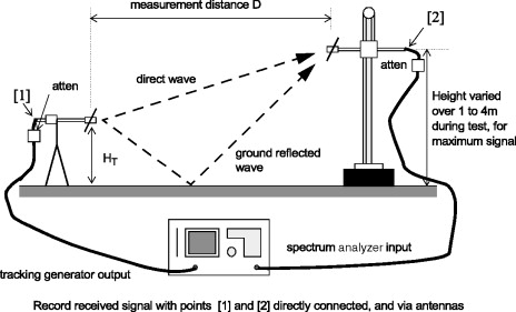
Site attenuation is the insertion loss measured between the terminals of two antennas on a test site, when one antenna is swept over a specified height range and both antennas have the same polarization. This gives an attenuation value in decibels at each frequency for which the measurement is performed. Transmit and receive antenna factors are subtracted from this value to give the normalized site attenuation (NSA), which should be an indication only of the performance of the site, without any relation to the antennas or instrumentation.
NSA measurements are performed for both horizontal and vertical polarizations, with the transmit antenna positioned at a height of 1 m (for broadband antennas) and the receive antenna swept over the appropriate height scan. CISPR standards specify a height scan of 1 to 4 m for 3-m and 10-m sites. The purpose of the height scan, as in the test proper (Section 23.2), is to ensure that nulls caused by destructive addition of the direct and ground reflected waves are removed from the measurement. Note that the height scan is not intended to measure or allow for elevation-related variations in signal emitted directly from the source, either in the NSA measurement or in a radiated emissions test.
Figure 22.17 shows the geometry and the basic method for an NSA calibration. Referring to that diagram, the procedure is to record the signal with points [1] and [2] connected, to give VDIRECT, and then via the antennas over the height scan, to give VSITE. Then NSA in decibels is given by (22.5)
![]() where AFT and AFR are the antenna factors.
where AFT and AFR are the antenna factors.
Figure 22.17. Geometry and setup for an NSA measurement.
CISPR 16-1-4, and related standards, includes the requirement that “A measurement site shall be considered acceptable when the measured vertical and horizontal NSAs are within ±4 dB of the theoretical normalized site attenuation” and goes on to give a table of theoretical values versus frequency for each geometry and polarization (the values differ between horizontal and vertical because of the different ground reflection coefficients). This is the yardstick by which any actual site is judged; the descriptions in Section 22.3.1.1 indicate how this criterion might be achieved, but as long as it is achieved, any site can be used for compliance purposes. Vice versa, a site that does not achieve the ±4-dB criterion cannot be used for compliance purposes no matter how well constructed it is. Note that the deviation from the theoretical values cannot be used as a “correction factor” to “improve” the performance of a particular site. This is because the NSA relates to a specific emitting source, and the site attenuation characteristics for real equipment under test may be quite different.
In choosing the ±4-dB criterion, it is assumed by CISPR that the instrumentation uncertainties (due to antenna factors, signal generator and receiver, cables, etc.) account for three quarters of the total and that the site itself can be expected to be within ±1 dB of the ideal. This has a crucial implication for the method of carrying out an NSA measurement. If you reduce the instrumentation uncertainties as far as possible you can substantially increase the chances of a site being found acceptable. Conversely, if your method has greater uncertainties than allowed for in the table, even a perfect site will not meet the criterion. Clearly, great attention must be paid to the method of performing an NSA calibration. The important aspects are
- Antenna factors—suitable for the geometry of the method, not free space
- Antenna balance and cable layout—to minimize the impact of the antenna cables
- Impedance mismatches—use attenuator pads on each antenna to minimize mismatch error
22.3.1.3. Radiated Measurements in a Screened Chamber
Open-area sites have two significant disadvantages, particularly in a European context—ambient radiated signals and bad weather. Ambients are discussed again in Section 23.5.2.5. These disadvantages create a preference for using sheltered facilities, and in particular screened chambers.
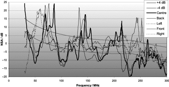
Alternative sites to the standard CISPR open-area test site are permitted provided that errors due to their use do not invalidate the results. As you might expect, their adequacy is judged by performing an NSA measurement. However, an extra requirement is added, which is to insist that the NSA is checked over the volume to be occupied by the largest EUT. This can require up to 20 separate NSA sweeps—five positions in the horizontal plane (center, left, right, front, and back) with two heights and for two polarizations each. As before, the acceptability criterion is that none of the measurements shall exceed ±4 dB from the theoretical.
The problem with untreated screened chambers for radiated measurements is that reflections occur from all six surfaces and will substantially degrade the site attenuation from EUT to measuring antenna (Hayward, Wickenden, and Aquila, 1995). For any given path, significant nulls and peaks with amplitude variations easily exceeding 30 dB will exist at closely spaced frequency intervals. Equally important, different paths will show different patterns of nulls and peaks, and small changes within the chamber can also change the pattern, so there is no real possibility of correcting for the variations. If you have to look for radiated emissions within a screened chamber, do it on the basis that you will be able to find frequencies at which emissions exist, but will not be able to draw any firm conclusions as to the amplitude of those emissions.
To be able to make anything approaching measurements in a screened chamber, the wall and ceiling reflections must be damped. The floor remains reflective, since the test method relies on the ground plane reflection, and so this kind of chamber is called semi-anechoic. This is achieved by covering these surfaces with radio absorbing material (RAM). RAM is available as ferrite tiles, carbon-loaded foam pyramids, or a combination of both, and it is quite possible to construct a chamber using these materials that meets the volumetric NSA requirement of ±4 dB. Enough such chambers have been built and installed that there is plenty of experience on call to ensure that this is achieved. The snag is that either material is expensive and will at least double the cost of the installed chamber. A comparison between the advantages and disadvantages of the three options is given in Table 22.2.
Table 22.2. Comparison of absorber materials
| Ferrite tiles | Pyramidal foam | Hybrid | |
|---|---|---|---|
| Size | No significant loss of chamber volume | Substantial loss of chamber volume | Some loss of chamber volume |
| Weight | Heavy; requires ceiling reinforcement | Reinforcement not needed | Heavy; requires ceiling reinforcement |
| Fixing | Critical—no gaps, must be secure | Not particularly critical | Critical—no gaps, must be secure |
| Durability | Rugged, no fire hazard, possibility of chipping | Tips can be damaged, possible fire hazard; can be protected | Some potential for damage and fire |
| Performance | Good mid-frequency, poor at band edges | Good at high frequency, poor at low frequency | Can be optimized across whole frequency range |
Partial lining of a room is possible but produces partial results (Bakker, Pues, and Grace, 1990; Dawson and Marvin, 1988). It may, though, be an option for precompliance tests. Figure 22.18 shows an example of a chamber NSA that falls substantially outside the required criterion but is still quite a lot better than a totally unlined chamber.
Figure 22.18. Example of a poor chamber NSA (vertical polarization, 1-m height).
The FAR Proposal
So far, we have discussed chambers that mimic the characteristics of an open-area site, that is, they employ a reflective ground plane and a height scan. This makes them a direct substitute for an OATS, allows them to be used in exactly the same way for the same standards, and generally avoids the question of whether the OATS is the optimum method for measuring radiated emissions.
In fact, it is not. It was originally proposed as a means of dealing with the unavoidable proximity of the ground in practical test setups, in the United States, where difficulties with ambient signals and the weather are less severe than in Europe. However, developments over the past 10 years in absorber materials have made it quite practical and cost effective to construct a small fully anechoic room (FAR), that is, with absorber on the floor as well, which can meet the volumetric ±4-dB NSA criterion. This environment is as near to free space as can be achieved. Its most crucial advantage is that, because there is no ground plane, there is no need for an antenna height scan. This eliminates a major source of uncertainty in the test (see Section 23.5) and generally allows for a faster and more accurate measurement.
Considerable work has been put in during the last few years to develop a standard for defining the test method in a FAR, and the detailed criteria that must be met by the room itself. This resulted in a European document, prEN 50147-3, which was never published but handed over to CISPR. It has eventually appeared as a combination of an amendment to CISPR 16-1-4 (CISPR, 2004, which describes the validation of the FAR) and another to CISPR 16-2-3 (CISPR, 2006, which describes the test method). Since it will have to coexist with the standard CISPR test method for some time to come, much of the concern surrounding its development has been to ensure as far as possible that it produces results that are comparable to the OATS method, which means that the necessary adjustment to the limit levels (because of the elimination of the reflected signal) is carefully validated and that the termination of the off-site cables is dealt with in an appropriate way. Neither of these documents sets emissions limits.
22.3.1.4. Conducted Emissions
By contrast with radiated emissions, conducted measurements need the minimum of extra facilities. The only vital requirement is for a ground plane of at least 2 m × 2 m, extending at least 0.5 m beyond the boundary of the EUT. It is convenient but not essential to make the measurements in a screened enclosure, since this will minimize the amplitude of extraneous ambient signals, and either one wall or the floor of the room can then be used as the ground plane. Non-floor-standing equipment should be placed on an insulating table 40 cm away from the ground plane.
Testing cable interference power with the absorbing clamp, as per EN55014-1, requires that the clamp should be moved along the cable by at least a half wavelength, which is 5 m at 30 MHz. This therefore needs a 5-m “racetrack” along which the cable is stretched; the clamp is rolled the length of the cable at each measurement frequency while the highest reading is recorded. There is no guidance in the standards as to whether the measurement should or should not be done inside a screened room. There are likely to be substantial differences one to the other, since the cable under test will couple strongly to the room and will suffer from room-induced resonances in the same manner as a radiated test, though to a lesser extent. For repeatability, a quasi-free-space environment would be better but will then suffer from ambient signals.
22.3.1.5. Precompliance and Diagnostic Tests
Full compliance with the EMC Directive can be achieved by testing and certifying to harmonized European standards. However the equipment and test facilities needed to do this are quite sophisticated and often outside the reach of many companies. The alternative is to take the product to be tested to a test house which is set up to do the proper tests, but this itself is expensive, and to make the best use of the time some preliminary if limited testing beforehand is advisable.
This consideration has given rise to the concept of “precompliance” testing. Precompliance refers to tests done on the production unit (or something very close to it) with a test setup and/or test equipment that may not fully reflect the standard requirements. The purpose is to
- Avoid or anticipate unpleasant surprises at the final compliance test
- Adequately define the worst-case EUT configuration for the final compliance test, hence saving time
- Substitute for the final compliance test if the results show sufficient margin
Diagnostics
Although you will not be able to make accurate radiated measurements in a laboratory environment, it is possible to establish a minimum setup in one corner of the lab at which you can perform emissions diagnostics and carry out comparative tests. For example, if you have done a compliance test at a test house and have discovered one particular frequency at 10 dB above the required limit, back in the lab you can apply remedial measures and check each one to see if it gives you a 15-dB improvement (5 dB margin) without being concerned for the absolute accuracy. While this method is not absolutely foolproof, it is often the best that companies with limited resources and facilities can do.
The following checklist suggests a minimum setup for doing this kind of in-house diagnostic work:
- Unrestricted floor area of at least 5 m × 3 m to allow a 3-m test range with 1 m beyond the antenna and EUT
- No other electronic equipment that could generate extraneous emissions (especially computers) in the vicinity—the EUT's support equipment should be well removed from the test area
- No mobile reflecting objects in the vicinity, or those that are mobile should have their positions carefully marked for repeatability
- An insulating table or workbench at one end of the test range on which to put the EUT, with a LISN bonded to the ground plane beneath it
- Equipment consisting of a spectrum analyzer, limiter, antenna set, and insulating tripod
- Antenna polarization generally horizontal, and the EUT cables stretched out horizontally and taped to the table facing it, since this reduces errors due to reflections and ground proximity
Once this setup is established it should not be altered between measurements on a given EUT. Since the antenna is at a fixed height, there should be no ground plane and the floor should not be metallic, since floor reflections should be attenuated as far as possible. This will give you a reasonable chance of repeatable measurements even if their absolute accuracy cannot be determined.
References
ANSI, 1988 ANSI Guide for Construction of Open Area Test Sites for Performing Radiated Emission Measurements 1988 ANSI C63.7-1988
Bakker et al., 1990 B.H. Bakker, H.F. Pues, N.V. Grace, A Novel Technique for Damping Site Attenuation Resonances in Shielding Semi-Anechoic Rooms IEE Seventh International Conference on EMC, York, UK, August 28–31 1990119-124
Bergervoet and van Veen., 1989 J.R. Bergervoet, H. van Veen., A Large Loop Antenna for Magnetic Field Measurements Eighth International EMC Symposium, Zurich, March 1989 1989
Bronaugh, 1986 E.L. Bronaugh, EMCO Scan Speed Limits in Automated EMI Measurements IERE Fifth International Conference on EMC, York, UK 1986
Bronaugh and Osburn, 1991 E.L. Bronaugh, J.D.M. Osburn, EMCO Radiated Emissions Test Performance of the GHz TEM Cell IEEE 1991 International Symposium on EMC, Cherry Hill, NJ, August 1991 1991
CISPR, no date CISPR. (no date) CISPR 16-1-X Specification for Radio Disturbance and Immunity Measuring Apparatus and Methods. Part 1. Radio disturbance and Immunity Measuring Apparatus.
CISPR, 2004 CISPR CISPR 16-1-4 Ed 1.0 A1: 2004 Amendment to CISPR 16-1-4 New Clause 5.8: Test Site Suitability without Ground Plane 2004
CISPR., 2005 CISPR CISPR/A/628/CD October 2005 (CISPR 16-1-1 Amd.2 f2 Ed.1.0): Weighting of Interference According to Its Effect on Digital Communication Services 2005
CISPR, 2006 CISPRCISPR 16-2-3 Ed.2: 2006 Specification for Radio Disturbance and Immunity Measuring Apparatus and Methods. Parts 2–3 Methods of Measurement of Disturbances and Immunity—Radiated Disturbance Measurements 2006
CISPR., 2006 CISPR CISPR/A/654/FDIS March 2006 Amendment 2 to CISPR 16-1-2 Ed.1: Update of LISN (Line Impedance Stabilization Network) Specifications 2006
DeMarinis, 1989 J. DeMarinis, DEC Getting Better Results from an Open Area Test Site DEC Eighth Symposium on EMC, Zurich, March 1989 1989
EMC Test Laboratories Association EMC Test Laboratories Association. (no date) “Emissions Tests on Telecom Ports as per CISPR 22 (EN 55022).” Technical Guidance Note TGN 42, available from www.emctla.co.uk.
Ettles, 1990 S.J. Ettles, British Telecom A Cost Effective Path to Electromagnetic Compatibility EMC 90—The Achievement of Compatibility, ERA Technology Conference Proceedings 90-0089, July 1990 1990
Hayward and Wickenden, 1995 A.C. Hayward, C. Wickenden, D.R.A. Aquila, Radiated Emission Measurements inside Shielded Enclosures IEE Colloquium on EMC Tests in Screened Rooms, April 11, 1995 IEE Colloquium Digest 1995 1995/074
IEC, no date IEC. (no date) IEC 61000-4-20: Electromagnetic Compatibility (EMC)—Part 4-20: Testing and Measurement Techniques—Emission and Immunity Testing in Transverse Electromagnetic (TEM) Waveguides, available at www.iec.ch.
Jackson, 1989 G.A. Jackson, ERA TechnologySurvey of EMC Measurement Techniques Electronics and Communication Engineering Journal (March/April) 198961-70
Jennings and Kwan,, 1986 W. Jennings, H. Kwan, DTI On the Design and Use of the Average Detector in Interference Measurement Fifth International Conference on EMC, York, UK, IERE Conf. Pub. 71 1986
Linkwitz, 1991 S. Linkwitz, Hewlett PackardAverage Measurements using a Spectrum Analyzer EMC Test and Design (May/June) 199134-38
Maas and Hoolihan, 1989 J.S. Maas, D.D. Hoolihan, IBMThe Effects of Ground Screen Termination on OATS Site Attenuation IEEE 1989 National Symposium on EMC, Denver, May 1989 1989
Nothofer, 2005 A. Nothofer, ... National Physical Laboratory/York EMC ServicesThe Use of GTEM Cells for EMC Measurement NPL Measurement Good Practice Guide 2005 available from publications page at www.npl.co.uk
Paul and Hardin, 1988 C.R. Paul, K.B. Hardin, IBM Diagnosis and Reduction of Conducted Noise Emissions International Symposium on EMC, IEEE, Washington, DC, August 2–4, 1988 1988
Porter, 1994 S.J. Porter, ... University of York A Comparison of Emissions Measurements in GTEM Cells with Open-Area Test Sites and Semi-Anechoic Chambers IEE Ninth International Conference on EMC, Manchester, UK, September 5–7, 1994 1994
Stecher, 1995 M. Stecher, Faster RFI Field-Strength Measurements through Prescanning with MDS Clamp News from Rohde and Schwarz no 1995147-
Wilson et al., 1989 P. Wilson, D. Hansen, D. Koenigstein, ABB Simulating Open Area Test Site Emission Measurements Based on Data Obtained in a Novel Broadband TEM Cell IEEE 1989 National Symposium on EMC, Denver, May 1989 1989