Chapter 16. Synthetic Instruments

The way electronic measurement instruments are built is making an evolutionary leap to a new method of design called synthetic instruments. This promises to be the most significant advance in electronic test and instrumentation since the introduction of automated test equipment (ATE). The switch to synthetic instruments is beginning now, and it will profoundly affect all test and measurement equipment that will be developed in the future.

Synthetic instruments are like ordinary instruments, in that they are specific to a particular measurement or test. They might be a voltmeter that measures voltage or a spectrum analyzer that measures spectra. The difference is that synthetic instruments are implemented purely in software that runs on general-purpose, nonspecific measurement hardware with a high-speed A/D or D/A converter at its core. In a synthetic instrument, the software is specific; the hardware is generic. Therefore, the personality of a synthetic instrument can be changed in an instant. A voltmeter may be a spectrum analyzer a few seconds later, and then become a power meter, or network analyzer, or oscilloscope. Totally different instruments are realized on the same hardware, switching back and forth in the blink of an eye, or even existing simultaneously.

The union of the hardware and software that implement a set of synthetic instruments is called a synthetic measurement system (SMS). This chapter studies both synthetic instruments and systems from which they may be best created.

Powerful customer demands in the private and public sectors are driving this change to synthetic instruments. There are many bottom-line advantages in making one, generic, and economical SMS hardware design do the work of an expensive rack of different, measurement-specific instruments. ATE customers all want to reap the savings this promises. ATE vendors like Teradyne, as well as conventional instrumentation vendors like Agilent and Aeroflex, have announced or currently produce synthetic instruments. The U.S. military, one of the largest ATE customers in the world, wants new ATE systems to be implemented with synthetic instruments. Commercial electronics manufacturers such as Lucent, Boeing, and Loral are using synthetic instruments now in their factories.

Despite the fact that this change to synthetic instrumentation is inevitable and widely acknowledged throughout the ATE and T&M (test and measurement) industries, there is a paucity of information available on the topic. A good deal of confusion exists about basic concepts, goals, and trade-offs related to synthetic instrumentation. Given that billions of dollars in product sales hang in the balance, it is important that clear, accurate information be readily available.

16.1. What Is a Synthetic Instrument?

Engineers often confuse synthetic measurement systems with other sorts of systems. This confusion is not because synthetic instrumentation is an inherently complex concept or because it is vaguely defined, but rather because there are lots of companies trying to sell their old nonsynthetic instruments with a synthetic spin.

If all you have to sell are pigs, and people want chickens, gluing feathers on your pigs and taking them to market might seem to be an attractive option to some people. If enough people do this, and feathered pigs, goats, cows, as well as turkeys and pigeons are flooding the market, being sold as if they were chickens, real confusion can arise among city folk regarding what a chicken might actually be.

One of the main purposes of this chapter is to set the record straight. When you are finished reading it, you should be able to tell a synthetic instrument from a traditional instrument. You will then be an educated consumer. If someone offers you a feathered pig in place of a chicken, you will be able to tell that you are being duped.

16.2. History of Automated Measurement

Purveyors of synthetic instrumentation often talk disparagingly about traditional instrumentation. But what exactly are they talking about? Often you will hear a system criticized as “traditional rack-em-stack-em.” What does that mean?

In order to understand what is being held up for scorn, you need to understand a little about the history of measurement systems.

16.2.1. Genesis

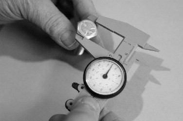
In the beginning, when people wanted to measure things, they grabbed a specific measurement device that was expressly designed for the particular measurement they wanted to make. For example, if they wanted to measure a length, they grabbed a scale, or a tape measure, or a laser range finder and carried it over to where they wanted to measure a length (Figure 16.1). They used that specific device to make their specific length measurement. Then they walked back and put the device away in its carrying case or other storage, and put it back on some shelf somewhere where they originally found it (assuming they were tidy).

Figure 16.1. Manual measurements.

If you had a set of measurements to make, you needed a set of matching instruments. Occasionally, instruments did double duty (a chronometer with built-in compass), but fundamentally there was a one-to-one correspondence between the instruments and the measurementsmade.

That sort of arrangement worksfine when you have only a few measurements to make, and you are not in a hurry. Under those circumstances, you do not mind taking the time to learn how to use each sort of specific instrument, and you have ample time todo everything manually, finding, deploying,using, and stowing the instrument.

Things went along like this for many centuries. But then in the 20th century, the pace picked up a lot. The minicomputer was invented, and people started using these inexpensivecomputers to control measurement devices. Using a computer to make measurements allows measurements to be made faster, and it allows measurements to be made by someone that might not know too much about how to operate the instruments. The knowledge for operating the instruments is encapsulated in software that anybody can run.

With computer-controlled measurement devices, you still needed a separate measurement device for each separate measurement. It seemed fortunate that you did not necessarily need a different computer for each measurement. Common instrument interface buses, like the IEEE-488 bus, allowed multiple devices to be controlled by a single computer. In those days, computers were still expensive, so it helped matters to economize on the number of computers.

And, obviously, using a computer to control measurement devices through a common bus requires measurement devices that can be controlled by a computer in this manner. An ordinary schoolchild's ruler cannot be easily controlled by a computer to measure a length. You needed a digitizing caliper or some other sort of length measurement device with a computer interface.

Things went along like this for a few years, but folks quickly got tired of taking all those instruments off the shelf, hooking them up to a computer, running their measurements, and then putting everything away. Sloppy, lazy folks that did not put their measurement instruments away tripped over the interconnecting wires. Eventually, somebody came up with the idea of putting all these computer-controlled instruments into one big enclosure, making a measurement system that comprised a set of instruments and a controlling computer mounted in a convenient package. Typically, EIA standard 19" racks were used, and the resulting sorts of systems have been described as “rack-em-stack-em” measurement systems. Smaller systems were also developed with instruments plugged into a common frame using a common computer interface bus, but the concept is identical.

At this point, the people that made measurements were quite happy with the situation. They could have a whole slew of measurements made with the touch of a button. The computer would run all the instruments and record the results. There was little to deploy or stow. In fact, since so many instruments were crammed into these rack-em-stack-em measurement systems, some systems got so big that you needed to carry whatever you were measuring to the measurement system, rather than the other way around. But that suited measurement makers just fine.

On the other hand, the people that paid for these measurement systems (seldom the same people as using them) were somewhat upset. They did not like how much money these systems were costing, how much room they took up, how much power they used, and how much heat they threw off. Racking up every conceivable measurement instrument into a huge, integrated system cost a mint and it was obvious to everyone that there were a lot of duplicated parts in these big racks of instruments.

16.2.2. Modular Instruments

As I referred to previously, there was an alternative kind of measurement system where measurement instruments were put into smaller, plug-in packages that connected to a common bus. This sort of approach is called modular instrumentation. Since this is essentially a packaging concept rather than any sort of architecture paradigm, modular instruments are not necessarily synthetic instrumentation at all. In fact, they usually are not, but since some of the advantages of modular packaging correspond to advantages of synthetic system design, the two are often confused.

Modular packaging can eliminate redundancy in a way that seems the same as how synthetic instruments eliminate redundancy. Modular instruments are boiled down to their essential measurement-specific components, with nonessential things like front panels, power supplies, and cooling systems shared among several modules.

Modular design saves money in theory. In practice, however, cost savings are often not realized with modular packaging. Anyone attempting to specify a measurement or test system in modular VXI packaging knows that the same instrument in VXI often costs more than an equivalent stand-alone instrument. This seems absurd given the fact that the modular version has no power supply, no front panel, and no processor. Why this economic absurdity occurs is more of a marketing question than a design optimization paradox, but the fact remains that modular approaches, although the darling of engineers, do not save as much in the real world as you would expect.

One might be tempted to point at the failure of modular approaches to yield true cost savings and predict the same sort of cost savings failure for synthetic instrumentation. The situation is quite different, however. The modular approach to eliminating redundancy and reducing cost does not go nearly as far as the synthetic instrument approach does. A synthetic instrument design will attempt to eliminate redundancy by providing a common instrument synthesis platform that can synthesize any number of instruments with little or no additional hardware. With a modular design, when you want to add another instrument, you add another measurement-specific hardware module. With a synthetic instrument, ideally you add nothing but software to add another instrument.

16.3. Synthetic Instruments Defined

Synergy means behavior of whole systems unpredicted by the behavior of their parts taken separately. —R. Buckminster Fuller (1975)

16.3.1. Fundamental Definitions

• Synthetic measurement system A synthetic measurement system is a system that uses synthetic instruments implemented on a common, general-purpose, physical hardware platform to perform a set of specific measurements.
• Synthetic instrument A synthetic instrument (SI) is a functional mode or personality component of a synthetic measurement system that performs a specific synthesis or analysis function using specific software running on generic, nonspecific physical hardware.

There are several key words in these definitions that need to be emphasized and further amplified.

16.3.2. Synthesis and Analysis

Although the word synthetic in the phrase synthetic instrument might seem to indicate that synthetic instruments are synthesizers—that they do synthesis, this is a mistake. When I say synthetic instrument, I mean that the instrument is being synthesized. I am not implying anything about what the instrument itself does.

A synthetic instrument might indeed be a synthesizer, but it could just as easily be an analyzer, or some hybrid of the two.

I have heard people suggest the term analytic instruments rather than synthetic instruments in the context of some analysis instrument built with a synthetic architecture, and this is not really correct either. Remember, you are synthesizing an instrument; the instrument itself may synthesize something, but that is another matter.

16.3.3. Generic Hardware

Synthetic instruments are implemented on generic hardware. This is probably the most salient characteristic of a synthetic instrument. It is also one of the bitterest pills to swallow when adopting an SI approach to measurements. Generic means that the underlying hardware is not explicitly designed to do the particular measurement. Rather, the underlying hardware is explicitly designed to be general purpose. Measurement specificity is encapsulated in software.

An exact analogy to this is the relationship between specific digital circuits and a general-purpose CPU (Figure 16.2). A specific digital circuit can be designed and hardwired with digital logic parts to perform a specific calculation. Alternatively, a microprocessor (or, better yet, a gate array) could be used to perform the same calculation using appropriate software. One case is specific, the other generic, with the specificity encapsulated in software.

Figure 16.2. Digital hardwired logic versus CPU.

The reason this is such a bitter pill is that it moves many instrument designers out of their hardware comfort zone. The orthodox design approach for instrumentation is to design and optimize the hardware so as to meet all measurement requirements. Specifications for measurement systems reflect this optimized-hardware orientation. Software is relegated to a subordinate role of collecting and managing measurement results, but no fundamental measurement requirements are the responsibility of any software.

With a synthetic instrumentation approach, the responsibility for meeting fundamental measurement requirements is distributed between hardware and software. In truth, the measurement requirements are now primarily a system-level requirement, with those high-level requirements driving lower-level requirements. If anything, the result is that more responsibility is given to software to meet detailed measurement requirements. After all, the hardware is generic. As such, although there will be some broad-brush optimization applied to the hardware to make it adequate for the required instrumentation tasks, the ultimate responsibility for implementing detailed instrumentation requirements belongs to software.

Once system planners and designers understand this point, it gives them a way out of a classic dilemma of test system design. I have seen many first attempts at synthetic instrumentation where this was not understood.

In these misguided efforts, the hardware designers continued to bear most or all of the responsibility for meeting system-level measurement performance requirements. Crucial performance aspects that were best or only achievable in system software were assigned to hardware solutions, with hardware engineers struggling against their own system design and the laws of physics to make something of the impossible hand they had been dealt. Software engineers habitually ignore key measurement performance issues under the invalid assumption that “the hardware does the measurement.” Software engineers focus instead on well-known TPS issues (configuration management, test executive, database, presentation, user interface [UI], and so forth), which are valid concerns but that should not be their only concerns.

One of the goals of this chapter is to raise awareness of this fact to people contemplating the development of synthetic instrumentation: A synthetic instrument is a system-level concept. As such, it needs a balanced system-level development effort to have any chance of being successful. Do not fall into the trap of turning to hardware as the solution for every measurement problem. Instead, synthesize the solution to the measurement problem using software and hardware together.

Organizations that develop synthetic instruments should make sure that the proper emphasis is placed. System-level goals for synthetic instruments are achieved by software. Therefore, the system designer should have a software skill set and be intimately involved in the software development. When challenges are encountered during design or development, software solutions should be sought vigorously, with hardware solutions strongly discouraged. If every performance specification shortfall is fixed by a hardware change, you know you have things backward.

16.3.4. Dilemma—All Instruments Created Equal

When the Founding Fathers of the United States wrote into the Declaration of Independence the phrase “all men are created equal,” it was clear to everyone then, and still should be clear to everyone now, that this statement is not literally true. Obviously, there are some tall men and some short men; men differ in all sorts of qualities. Half the citizens to which that phrase refers are actually women.

What the Founding Fathers were doing was to establish a government that would treat all of its citizens as if they were equal. They were perfectly aware of the inequalities between people, but they felt that the government should be designed as if citizens were all equivalent and had equivalent rights. The government should be blind to the inherent and inevitable differences between citizens.

Doubtless, the resources of government are always limited. Some citizens who are extremely unequal to others may find that their rights are altered from the norm. For example, an 8-ft tall man might find some difficulty navigating most buildings, but the government would find it difficult to mandate that doorways all be taller than 8 ft.

Thus, a consequence of the “created equal” mandate is that the needs of extreme minorities are neglected. This is a dilemma. Either one finds that extraordinary amounts of resources are devoted to satisfying these minority needs, which is unfair to the majority, or the needs of the minority are sacrificed to the tyranny of the majority. The endless controversies that result are well known in U.S. history.

You may be wondering where I am going with this digression on U.S. political thought and why it has any place in a book about synthetic instrumentation. Well, the same sort of political philosophy characterizes the design of synthetic instrumentation and synthetic measurement systems. All instruments are created equal by the fiat of the synthetic instrument design paradigm. That means, from the perspective of the system designer, that the hardware design does not focus on and optimize the specific details of the specific instruments to be implemented. Rather, it considers the big picture and attempts to guarantee that all conceivable instruments can flourish with equal “happiness.”

But we all know that instruments are not created equal. As with government, there are inevitable trade-offs in trying to provide a level playing field for all possible instruments. Some types of instruments and measurements require far different resources than others. Attempting to provide for these oddball measurements will skew the generic hardware in such a way that it does a bad job supporting more common measurements.

Here is an example. Suppose there is a need for a general-purpose test and measurement system that would be able to test any of a large number of different items of some general class and determine if they work. An example of this would be something like a battery tester. You plug your questionable battery into the tester, push a button, and a green light illuminates (or meter deflects to the green zone) if the battery is good or red if bad.

But suppose that it was necessary to test specialized batteries, like car batteries, or high-power computer UPS batteries, or tiny hearing aid batteries. Nothing in a typical consumer battery tester does a good job of this. To legitimately test big batteries you would want to have a high-power load, cables thick enough to handle the current, and so on. Small batteries need tiny connectors and sockets that fit their various shapes. Adding the necessary parts to make these tests would drive up the cost, size, and other aspects of the tester.

Thus, there seems to be an inherent compromise in the design of a generic test instrument. The dilemma is to accept inflated costs to provide a foundation for rarely needed, oddball tests or to drop the support for those tests, sacrificing the ability to address all test needs.

Fortunately, synthetic instrumentation provides a way to break out of this dilemma to some degree—a far better way than traditional instrumentation provided. In a synthetic instrumentation system, there is always the potential to satisfy a specific, oddball measurement need with software. Although software always has costs (both nonrecurring and recurring), it is most often the case that handling a minority need with software is easier to achieve than it is with hardware.

A good, general example of this is how digital signal processing (DSP) can be applied in postprocessing to synthesize a measurement that would normally be done in real time with hardware. A specific case would be demodulating some form of encoding. Rather than include a hardware demodulator in order to perform some measurement on the encoded data, DSP can be applied to the raw data to demodulate in postprocessing. In this way, a minority need is addressed without adding specialized hardware.

Continuing with this example, if it turns out that DSP postprocessing does not have sufficient performance to achieve the goal of the measurement, one option is to upgrade the controller portion of the control, codec, conditioning (CCC) instrument. Maybe then the DSP will run adequately. Yes, the hardware is now altered for the benefit of a single test but not by adding hardware specific to that test. This is one of my central points. As I will discuss in detail later on, I believe it is a mistake to add hardware specific to a particular test.

16.4. Advantages of Synthetic Instruments

No one would design synthetic instruments unless there was an advantage, above all, a cost advantage. In fact, there are several advantages that allow synthetic instruments to be more cost effective than their nonsynthetic competitors.

16.4.1. Eliminating Redundancy

Ordinary rack-em-stack-em instrumentation contains repeated components. Every measurement box contains a slew of parts that also appear in every other measurement box. Typical repeated parts include

• Power supply
• Front panel controls
• Computer interfaces
• Computer controllers
• Calibration standards
• Mechanical enclosures
• Interfaces
• Signal processing

A fundamental advantage of a synthetic approach to measurement system design is that adding a new measurement does not imply that you need to add another measurement box. If you do add hardware, the hardware comes from a menu of generic modules. Any specificity tends to be restricted to the signal conditioning needed by the sensor or effector being used.

16.4.2. Stimulus Response Closure: The Calibration Problem

Many of the redundancies eliminated by synthetic instrumentation are the same as redundancies eliminated by modular instrument approaches. However, one significant redundancy that synthetic instruments have the unique ability to eliminate is the response components that are responsible for stimulus and the stimulus components that support response. I call this efficiency closure. I will show, however, that this sort of redundancy elimination, while facilitated by synthetic approaches, has more to do with using a system-level optimization rather than an instrument-level optimization.

A signal generator (a box that generates an AC sine wave at some frequency and amplitude) is a typical stimulus instrument that you may encounter in a test system. When a signal generator creates the stimulus signal, it must do so at a known, calibrated signal level. Most signal generators achieve this by a process called internal leveling. The way internal leveling is implemented is to build a little response measurement system inside the signal generator. The level of the generator is then adjusted in a feedback loop so as to set the level to a known, calibrated point.

As you can see in Figure 16.3, this stimulus instrument comprises not only stimulus components but also response measurement components. It may be the case that elsewhere in the overall system, those response components needed internally in the signal generator are duplicated in some other instruments. Those components may even be the primary function of what might be considered a “true” response instrument. If so, the response function in the signal generator is redundant.

Figure 16.3. Signal-generator leveling loop.

Naturally, this sort of redundancy is a true waste only in an integrated measurement system with the freedom to use available functions in whatever manner desired, combining as needed. A signal generator has to work stand-alone and so must carry a redundant response system within itself. Even a synthetic signal generator designed for stand-alone modular VXI or PXI use must have this response measurement redundancy within.

Therefore, it would certainly be possible to look at a system comprising a set of nonsynthetic instruments and to optimize away stimulus response redundancy. That would be possible, but it is difficult to do in practice. The reason it is difficult is that nonsynthetic instruments tend to be specific in their stimulus and response functions. It is difficult to match up functions and factor them out.

In contrast, when one looks at a system designed with synthetic stimulus and response components, the chance of finding duplicate functions is much higher. If synthetic functions are all designed with the same signal conditioner, converter, DSP subsystem cascade, then a response system provided in a stimulus instrument will have the same exact architecture as one provided in a response instrument. The duplications factor out directly.

16.4.3. Measurement Integration

One of the most powerful concepts associated with synthetic instrumentation is the concept of measurement integration.

16.4.3.1. Fundamental Definition

• Measurement integration Combining disparate measurements into a single measurement map.

Measurement can be developed in a way that encourages measurement integration. When you specify a list of ordinates and abscissas and state how the abscissas are sequenced, you have effectively packaged a bunch of measurements into a tidy bundle. This is measurement integration in its purest sense.

Measurement integration is important because it allows you to get the most out of the data you take. The data set is seen as an integrated whole that is analyzed, categorized, and visualized in whatever way makes the most sense for the given test. This is in contrast with the more prevalent way of approaching test where a separate measurement is done in a sequential process with each test. There is no intertest communication (beyond basic prerequisites and an occasional parameter). The result of this redundancy is slow testing and ambiguity in the results.

16.4.4. Measurement Speed

Synthetic instruments are unquestionably faster than ordinary instruments. There are many reasons for this fact, but the principal reason is that a synthetic instrument does a measurement that is exactly tuned to the needs of the test being performed: nothing more, nothing less. It does exactly the measurement that the test engineer wants.

In contrast, ordinary instruments are designed to a certain kind of measurement, but the way they do it may not be optimized for the task at hand. The test engineer is stuck with what the ordinary instrument has in its bag of tricks.

For example, there is a speed/accuracy trade-off on most measurements. If an instrument does not know exactly how much accuracy you need for a given test, it needs to take whatever time it takes for the maximum accuracy you might ever want. Consequently, you get the slowest measurement. It is true that many conventional instruments that make measurements with a severe speed/accuracy trade-off often have provision to specify a preference (e.g., a frequency counter that allows you to specify the count time and/or digits of precision), but the test engineer is always locked into the menu of compromises that the instrument maker anticipated.

Another big reason why synthetic instrumentation makes faster measurements is that the most efficient measurement techniques and algorithms can be used. Consider, for example, a common swept filter spectrum analyzer. This is a slow instrument when fine frequency resolution is required simultaneously with a wide span. In contrast, a synthetic spectrum analyzer based on fast Fourier transform (FFT) processing will not suffer a slowdown in this situation.

Decreased time to switch between measurements is also another noteworthy speed advantage of synthetic instrumentation. This ability goes hand-in-hand with measurement integration. When you can combine several different measurements into one, eliminating both the intermeasurement setup times and the redundancies between sets of overlapping measurements, you can see surprising speed increases.

16.4.5. Longer Service Life

Synthetic measurement systems do not become obsolete as quickly as less flexible dedicated measurement hardware systems. The reason for this fact is quite evident: Synthetic measurement systems can be reprogrammed to do both future measurements, not yet imagined, at the same time as they can perform legacy measurements done with older systems. Synthetic measurement systems give you your cake and allow you to eat it too, at least in terms of nourishing a wide variety of past, present, and future measurements.

In fact, one of the biggest reasons the U.S. military is so interested in synthetic measurement systems is this unique ability to support the old and the new with one, unchanging system. Millions of personnel-hours are invested in legacy test programs that expect to run on specific hardware. That specific hardware becomes obsolete. Now what do we do?

Rather than dumping everything and starting over, a better idea is to develop a synthetic measurement system that can implement synthetic instruments that do the same measurements as hardware instruments from the old system, while at the same time, are able to do new measurements. Best of all, the new SMS hardware is generic to the measurements. That means it can go obsolete piecemeal or in great chunks and the resulting hardware changes (if done right) do not affect the measurements significantly.

16.5. Synthetic Instrument Misconceptions

Now that you understand what a synthetic instrument is, let us tackle some of the common misconceptions surrounding this technology.

16.5.1. Why Not Just Measure Volts with a Voltmeter?

The main goal of synthetic instrumentation is to achieve instrument integration through the use of multipurpose stimulus/response synthesis/analysis hardware. Although there may be nonsynthetic, commercial off-the-shelf (COTS) solutions to various requirements, we intentionally eschew them in favor of doing everything with a synthetic CCC approach.

It should be obvious that a COTS, measurement-specific instrument that has been in production many years and has gone through myriad optimizations, reviews, updates, and improvements will probably do a better job of measuring the thing it was designed to measure than a first-revision synthetic instrument.

However, as the synthetic instrument is refined, there comes a day when the performance of the synthetic instrument rivals or even surpasses the performance of the legacy, single-measurement instrument. The reason this is possible is because the synthetic instrument can be continuously improved, with better and better measurement techniques incorporated, even completely new approaches. The traditional instrument cannot do that.

16.5.1.1. Synthetic Musical Instruments

This book is about synthetic measurement instruments, but the concept is not far from that of a synthetic musical instrument. Musical instrument synthesizers generate sound-alike versions f many classic instruments by means of generic synthesis hardware. In fact, the quality of the synthesis in synthetic musical instruments now rivals, and in some cases surpasses, the musical-aesthetic quality of the best classic mechanical musical instruments. Modern musical synthesis systems also can accurately imitate the flaws and imperfections in traditional instruments. This situation is exactly analogous to the eventual goal of synthetic instrument—that they will rival and surpass, as well as imitate, classic dedicated hardware instruments.

16.5.2. Virtual Instruments

In Section 16.2, History of Automated Measurement, I described automated, rack-em-stack-em systems. People liked these systems, but they were too big and pricey. As a consequence, modular approaches were developed that reduced size and presumably cost by eliminating redundancy in the design. These modular packaging approaches had an undesirable side effect: They made the instrument front panels tiny and crowded. Anybody that used modular plug-in instruments in the 1970s and 1980s knows how crowded some of these modular instrument front panels got (Figure 16.4).

Figure 16.4. Crowded front panel on Tektronix spectrum analyzer.

It occurred to designers that if the instrument could be fully controlled by computer, there might be no need for a crowded front panel. Instead, a soft front panel could be provided on a nearby PC that would serve as a way for a human to interact with the instrument. Thus, the concept of a virtual instrument appeared. Virtual instruments were actually conventional instruments implemented with a pure, computer-based user interface.

Certain software technologies, like National Instruments' LabVIEW product, facilitated the development of virtual instruments of this sort. The very name virtual instrument is deeply entwined with LabVIEW. In a sense, LabVIEW defines what a virtual instrument was and is.

Synthetic instruments running on generic hardware differ radically from ordinary instrumentation, where the hardware is specific to the measurement. Therefore, synthetic instruments also differ fundamentally from virtual instruments, where, again, the hardware is specific to a measurement. In this latter case, however, the difference is more disguised since a virtual instrument block diagram might look similar to a synthetic instrument block diagram. Some might call this a purely semantic distinction, but in fact, the two are quite different.

Virtual instruments are a different beast than synthetic instruments because virtual instrument software mirrors and augments the hardware, providing a soft front panel or managing the data flow to and from a conventional instrument in a rack, but does not start by creating or synthesizing something new from generic hardware.

This is the essential point: Synthetic instruments are synthesized. The whole is greater than the sum of the parts. To use Buckminster Fuller's words, synthetic instruments are synergistic instruments (1975). Just as a triangle is more than three lines, synthetic instruments are more than the triangle of hardware (control, codec, conditioning) they are implemented on.

Therefore, one way to tell if you have a true synthetic instrument is to examine the hardware design alone and to try to figure out what sort of instrument it might be. If all you can determine are basic facts, like the fact that it is a stimulus or response instrument, or like the fact that it might do something with signals on optical fiber, but not anything about what it is particularly designed to create or measure—if the measurement specificity is all hidden in software—then you likely have a synthetic instrument.

I mentioned National Instruments' LabVIEW product earlier in the context of virtual instruments. The capabilities of LabVIEW are tuned more toward an instrument stance rather than a measurement stance (at least at the time of this writing) and therefore do not currently lend themselves as effectively to the types of abstractions necessary to make flexible synthetic instrumentation as do other software tools. In addition, LabVIEW's non-object-oriented approach to programming prevents the application of powerful object-oriented (OO) benefits like efficient software reuse. Since OO techniques work well with synthetic instrumentation, LabVIEW's shortcoming in this regard represents a significant limitation.

That said, there is no reason that LabVIEW cannot be used to as a tool for creating and manipulating synthetic instruments, at some level. Just because LabVIEW is currently tuned to be a non-OO virtual instrument tool, does not mean that it cannot be a SI tool to some extent. Also, it should be noted that the C++-based LabWindows environment does not share as many limitations as the non-OO LabVIEW tools.

16.5.3. Analog Instruments

One common misconception about synthetic instruments is that they can be only analog measuring instruments. That is to say, they are not appropriate for digital measurements. Because of the digitizer, processing has moved from the digital world to the analog world, and what results is only useful for analog measurements.

Nothing could be further from the truth. All good digital hardware engineers know that digital circuitry is no less “analog” than analog circuits. Digital signaling waveforms, ideally thought of as fixed 1 and 0 logic levels are anything but fixed: they vary; they ring; they droop; they are obscured by glitches, spurs, hum, noise, and other garbage.

Performing measurements on digital systems is a fundamentally analog endeavor. As such, synthetic instrumentation implemented with a CCC hardware architecture is equally appropriate for digital test and analog test.

There is, without doubt, a major difference between the sorts of instruments that are synthesized to address digital versus analog measurement needs. Digital systems often require many more simultaneous channels of stimulus and response measurement than do analog systems. But bandwidths, voltage ranges, and even interfacing requirements are similar enough in enough cases to make the unified synthetic approach useful for testing both kinds of systems with the same hardware asset.

Another difference between analog- and digital-oriented synthetic measurement systems is the signal conditioning used. In situations where only the data is of interest, rather than the voltage waveform itself, the best choice of signal conditioner may be nonlinear. Choose nonlinear digital-style line drivers and receivers in the conditioner. Digital drivers will give us better digital waveforms, per dollar, than linear drivers. Similarly, when implementing many channels of response measurement, a digital receiver will be far less expensive than a linear response asset.

16.6. Synthetic Measurement System Hardware Architectures

The heart of the hardware system concept for synthetic instrumentation is a cascade of three subsystems: digital control and timing, analog/digital conversion (codec), and analog signal conditioning. The underlying assumption in the synthetic instrument concept is that this architecture concept is a good choice for the architecture of next-generation instrumentation. Next, I will explore the practical and theoretical implications of this concept. Other architectural options and concepts that relate to the fundamental concept will also be considered.

16.7. System Concept—The CCC Architecture

The cascade of three subsystems, control, codec, and conditioning, is shown in Figure 16.5.

Figure 16.5. Basic CCC cascade.

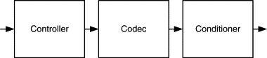
I will call this architecture the three C's or the CCC architecture: control, codec, and conditioning. In a stimulus asset, the controller generates digital signal data that is converted to analog form by the codec, which is then adjusted in voltage, current, bandwidth, impedance, coupling, or has any of a myriad of possible interface transformations performed by the conditioner.

16.7.1. Signal Flow

Thus, the “generic” hardware used as a platform for synthetic instrumentation comprises a cascade of three functional blocks. This cascade might flow either way, depending on the mode of operation. A sensor might provide a signal input for signal conditioning, analog-to-digital conversion (A/D), and processing, or alternatively, processing might drive digital-to-analog conversion (D/A), which drives signal conditioning to an effector.

In my discussions of synthetic instrumentation architecture, I will often treat digital-to-analog conversion as an equivalent to analog-to-digital conversion. The sense of the equivalence is that these two operations represent a coding conversion between the analog and digital portions of the system. The only difference is the direction of signal flow through them. This is exactly the same as how I will refer to signal conditioners as a generic class that comprises both stimulus (output) conditioners and response (input) conditioners (Figure 16.6).

Figure 16.6. Synthetic architecture cascade—flow alternatives.

Thus, in this book, when I refer to either of the two sorts of converters as an equivalent element in this sense, I will often call it a codec or converter, rather than be more restrictive and call it an A/D or a D/A. (Although the word codec implies both a coder and a decoder, I will also use this word to refer to either individually or collectively.) This will allow us to discuss certain concepts that apply to both stimulus and response instruments equally. Similarly, I will refer to signal conditioners and digital processors (controllers) generically as well as in a specific stimulus or response context.

16.7.2. The Synthetic Measurement System

When you put a stimulus and response asset together, with a device under test (DUT) in the middle, you now have a full-blown synthetic measurement system (Figure 16.7). (In the automated test community, engineers often use the jargon acronym DUT to refer to the device under test. Some engineers prefer unit under test [UUT]. Whatever you call it, DUT or UUT, it represents the “thing” you are making measurements about. Most often this is a physical thing, a system possibly. Other times it may be more abstract, a communications channel, for instance. In all cases, it is something separate from the measurement instrument.)

Figure 16.7. Synthetic measurement system.

16.7.3. Chinese Restaurant Menu (CRM) Architecture

When one tries to apply the CCC hardware architecture to a wide variety of measurement problems, it often becomes evident that practical limitations arise in the implementation of a particular subsystem with respect to certain measurements. For example, voltage ranges might stress the signal conditioner, or bandwidth might stress the codec, or data rates might stress the controller, and so on. Given this problem, the designer is often inclined to start substituting sections of hardware for different applications. With this approach taken, the overall system begins to comprise several CCC cascades, with portions connected as needed to generate a particular stimulus. Together they form a sort of “Chinese restaurant menu” of possibilities—CRM architecture for short (Figure 16.8).

Figure 16.8. CRM architecture.

To create an instrument hardware platform, select one item from column A (a signal conditioner), one item from column B (a codec asset), and one item from column C (a digital processor) to form a single CCC cascade from which to synthesize your instrument.

For example, consider the requirements for a signal generator versus a pulse generator. A pulse generator, unless it needs rise-time control, can get away with a “1-bit” D/A. Even with rise-time control, only a few bits are really needed if a selection of reconstruction filters are available. On the other hand, a high-speed pulse-timing controller is needed, possibly with some analog, fine-delay control, and the signal conditioning would be best done with a nonlinear pulse buffer with offset capability and specialized filtering for rise-/fall-time control.

In contrast, the signal generator fidelity requirements lead us to a finely quantized D/A, with at least 12 bits. A direct-digital-synthesis (DDS) oriented controller is needed to generate periodic waveforms; and a linear, low-distortion, analog buffer amplifier is mandatory for signal conditioning.

Therefore, when faced with requirements for a comprehensive suite of tests, one way to handle the diversity of requirements is to provide multiple choices for each of the “three C's” in the CCC architecture.

Table 16.1 is one possible menu. Column A is the control and timing circuitry, column B is the D/A codec, and column C is the signal conditioning. To construct a particular stimulus, you need to select appropriate functions from columns A, B, and C that all work together for your application.

Table 16.1. CRM architecture

Control and timing	Codec conversion	Signal conditioning
DSP or μP	1-bit (on/off) voltage source (100 GHz)	Nonlinear digital driver
High-speed state machine	18-bit, 100 kHz D/A	Wideband linear amplifier
Medium-speed state machine with RAM	12-bit, 100 MHz D/A	High-voltage amplifier
Parallel I/O board driven by TP	8-bit, 2.4 GHz D/A	Up-converter

The items from the CRM architecture can be selected on the spot by means of switches, or alternatively, stimulus modules can be constructed with hardwired selections from the menu. The choice of module can be specified in the measurement strategy, or it can be computed using some heuristic.

But the CRM design is somewhat of a failure; it compromises the goal of synthetic design. The goal of synthetic instrumentation design is to use a single hardware asset to synthesize any and all instruments. When you are allowed to pick and choose, even from a CRM of CCC assets, you have taken your first step down the road to hell—the road to rack-n-stack modular instrumentation. In the limit, you are back to measurement-specific hardware again, with all the redundancy put back in. Rats! And you were doing so well!

Let us take another look at the signal generator and pulse generator from the “pure” synthetic instrumentation perspective. Maybe you can save yourself.

16.7.4. Parameterization of CCC Assets

One way to fight the tendency to design with a CRM architecture is to use asset parameterization. Instead of swapping out a CCC asset completely, design the asset to have multiple modes or personalities so that it can meet multiple requirements without being totally replaced.

This sort of approach is not unlike the nonpolymorphic functional factorizations in procedural software, when type parameters are given to a function. Rather than making complete new copies of an asset with certain aspects of its behavior altered to fit each different application, a single asset is used with those changing performance aspects programmable based on its current type.

For example, rather than making several different signal conditioners with different bandwidths, make a single signal conditioner that has selectable bandwidth. To the extent that bandwidth can be parameterized in a way that does not require the whole asset to be replaced (equivalent to the CRM design), the design is now more efficient through its use of parameterization (Figure 16.9).

Figure 16.9. Parameterized architecture.

The choice between multiple modules with different capabilities and a single module with multiple capabilities is a design decision that must be made by the synthetic measurement system developers based on a complete view of the requirements. There is no way to say a priori what the right way is to factor hardware. The decision must be made in the context of the design requirements. However, it is important to be aware of the tendency to modularize and solve specific measurement issues by racking up more specific hardware, which leads away from the synthetic instrument approach.

16.7.5. Architectural Variations

Although in many circumstances there is good potential for the basic synthetic instrument architecture, one can anticipate that some architectural variations and options need to be considered. Sadly, many of these variations backslide to habitual, sanctioned approaches. There is nothing to be done about this; the realities of commercial development must be acknowledged.

The reasons synthetic instrument designers consider deviations from the pure “three C's” tend to be matters of realizability, cost, risk, or marketing. The state of the art is that a more conservative design approach is taken. And, for whatever reason, customers may simply want a different approach.

In this book, I will not bother to consider architecture variations that are expedient for reasons of risk or marketing, but I will mention a few variations that are wins with respect to cost and realizability. These tend to be SMS architectural enhancements rather than mere expedient hacks to get something built. Enhancements like compound stimulus and multiplexing are two of the most prominent.

16.7.6. Compound Stimulus

One architecture enhancement of CCC that is often used is called compound stimulus, where one stimulus is used in the generation of another stimulus. The situation to which this enhancement lends itself is whenever state-of-the-art D/A technology is inadequate, expensive, or risky to use to generate an encoded stimulus signal directly with a single D/A.

The classic example of compound stimulus is the use of an up-converter to generate a modulated bandpass signal waveform. This is accomplished by a combination of subsystems as shown in Figure 16.10.

Figure 16.10. Compound stimulus.

Note that the upper “synthesizer” block shows an internal structure that parallels the desired CCC structure of a synthetic instrument. The output of this synthesizer is fed down to the signal conditioning circuit of the lower stimulus system. The lower system generates the modulation that is up-converted to form the compound stimulus.

Whenever a signal encoding operation is performed, there will be an open input for either the encoded signal or the signal on which it is encoded. This is an opportunity for compound stimulus. Signal encoding is inherently a stimulus compounding operation.

In recognition of this situation, CCC assets can be deployed with a switch matrix that allows their outputs to be directed not only at DUT inputs, but alternatively to coding inputs on other CCC stimulus assets. This results in a CCC compound matrix architecture that allows us to deploy all assets for the generation of compound-encoded waveforms.

16.7.7. Simultaneous Channels and Multiplexing

An issue that is often ignored in the development of synthetic measurement systems is the need for multiple, simultaneous stimuli and multiple, simultaneous measurements. With many tests, a single stimulus is not enough. And although, most times, multiple responses can be measured sequentially, there are some cases where simultaneous measurement of response is paramount to the goal of the test.

Given this need, what do we do? The most obvious solution is to simply build more CCC channels. Duplicate the CCC cascade for stimulus as many times as needed so as to provide the required stimuli. Similarly, duplicate the response cascade to be able to measure as many responses as needed.

This obvious solution certainly can be made to work in many applications, but what may not be obvious is that there are other alternatives. There are other ways to make multiple stimuli and make multiple response measurements, without using completely duplicated channels. Moreover, it may be the case that duplicated channels cost more and have inferior performance as compared to the alternatives.

What are these cheaper, better alternatives? They all fall into a class of techniques called multiplexing. When you multiplex, you make one channel do the work of several. The way this is accomplished is by taking advantage of orthogonal modes in physical media. Any time uncoupled modes occur, you have an opportunity to multiplex.

There are various forms of multiplexing, each based on a set of modes used to divide the channels. The most common forms used in practice are the following:

• Space division multiplexing
• Time division multiplexing
• Frequency division multiplexing
• Code division multiplexing

These multiplexing techniques can be implemented in hardware, of course, but they can also be synthetically generated. After all, if you have the ability to generate any of a menu of synthetic instruments on generic hardware, why not synthesize multiple instruments simultaneously?

16.7.7.1. Space Division Multiplexing

Space division multiplexing (SDM) is a fancy name for multiple channels (Figure 16.11). Separate channels with physical separation in space is the orthogonal mode set. SDM has the unique advantage of being obvious and simple. If you want two stimuli, build two stimulus cascade systems. If you want two responses, build two response cascades. A more subtle advantage, but again unique to SDM and very important, is the fact that multiple SDM channels each have exactly the same bandwidth performance of a single channel. This may seem trivial, but it is not strictly true with other techniques. Another advantage of space multiplexing is that it tends to achieve good orthogonality. That is to say, there is little crosstalk between channels. What is generated/measured on one channel does not influence another.

Figure 16.11. Space division multiplexing.

But there are many significant disadvantages to space multiplexing. Foremost among these is the fact that N channels implemented with space multiplexing cost at least N times more than a single channel, sometimes more. Another prominent disadvantage of space multiplexing is a consequence of the good orthogonality: The channels are completely independent, they can drift independently. Thus, gain drift, offsets, and problems like phase and delay skew, among others, will all be worse in a space-multiplexed system.

16.7.7.2. Time Division Multiplexing

The most common alternative to space multiplexing is time division multiplexing (TDM). The TDM technique is based on the idea of using a multiway switch, often called a commutator, to divide a single channel into multiple channels in a time-shared manner (Figure 16.12).

Figure 16.12. Time division multiplexing.

Time multiplexing schemes are easy to implement, and to the extent that the commutator is inexpensive compared to a channel, a TDM approach can be far less expensive than most any other multiplexing approach. Another advantage is in using the same physical channel for each measurement or stimulus, there is less concern about interchannel drift or skew.

On the downside, a new concern becomes important: the speed of the commutator in relation to the bandwidth of the signals. Unlike SDM, where it is obvious that the multiple channels each work as well, bandwidthwise, as an individual channel, with TDM there may be a problem. The available single-channel bandwidth is shared among each multiplexed channel.

It can be shown (Carlson, 1968), however, that, if the commutator visits each channel at least at the Nyquist rate (twice the bandwidth of the channel), all information from each channel is preserved. This is a point that recurs in other multiplexing techniques. It turns out that for N channels TDM multiplexed to have the same bandwidth performance as a single channel with bandwidth B, they need to be multiplexed onto a single channel with bandwidth N times B at a minimum. Thus, TDM (and all other multiplexing techniques) are seen as a space/bandwidth trade-off.

TDM is relatively easy to implement synthetically. Commutation and decommutation are straightforward digital techniques that can be used exclusively in the synthetic realm or paired with specific commutating hardware. One possible architecture variation that uses a virtual commutator implemented synthetically is shown in Figure 16.13.

Figure 16.13. Time division multiplexing with virtual commutator.

The application of TDM shown in Figure 16.13 assumes a multiinput, single-output DUT. Multiplexing is used in a way that allows a single stimulus channel to make measurements of all the inputs. The corresponding responses are easily sliced apart in the controller.

16.7.7.3. Frequency Division Multiplexing

Another common alternative to space multiplexing is frequency division multiplexing (FDM). The FDM technique is based on the idea of using different frequencies, or subcarriers, to divide a single channel into multiple channels in a frequency allocated manner.

FDM schemes are somewhat harder to implement than TDM. Some sort of mixer is needed to shift the channels to their respective subcarriers. Later they must be filtered apart and unmixed. Modern DSP simplifies a lot of the issues that would otherwise make this technique more costly. Synthetic FDM is straightforward to achieve.

In Figure 16.14, three frequencies, F1, F2, and F3, are used with mixers to allow a single response channel to make simultaneous measurements of a DUT with three outputs. Within the controller, a filter bank implemented as an FFT separates the individual response signals.

Figure 16.14. Frequency division multiplexing.

Unfortunately, unlike TDM, even though the same physical channel is used for each measurement or stimulus, those signals occupy different frequency bands in the single physical channel. There is no guarantee that intermux-channel drift or skew will not occur. On the other hand, the portions of FDM implemented synthetically will not have this problem—or can correct for this problem in the analog portions.

Again it is true that, for N channels, FDM multiplexed, to have the same bandwidth performance as a single channel with bandwidth B, they must be multiplexed on a single channel with a bandwidth N times B, at a minimum.

16.7.7.4. Code Division Multiplexing

A more esoteric technique for multiplexing (although much more well known these days because of the rise of cellular phones that use CDMA) is code division multiplexing (CDM). The CDM technique is based on the idea of using different orthogonal codes, or basis functions, to divide a single channel into multiple channels along orthogonal axes in code space.

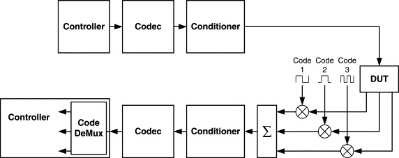
To the first order, CDM schemes are of the same complexity as FDM techniques, so the two methods are often compared in terms of cost and performance. The frequency mixer used in FDM is used the same way in CDM, this time with different codes rather than frequencies. Again, fancy DSP can be used to implement synthetic CDM. Separate code multiplexed channels can be synthesized and demultiplexed with DSP techniques. Figure 16.15 shows a CDM system that achieves the same multiplexing as the FDM system in Figure 16.14.

Figure 16.15. Code division multiplexing.

As with TDM, because the same physical channel is used for each measurement or stimulus, there is less concern about interchannel drift or skew. Unlike FDM, codes will spread each channel across the same frequencies. In fact, CDM has the unique ability to ameliorate some frequency-related distortions that plague all other techniques, including space multiplexing.

Again it is true that, for N channels, CDM multiplexed, to have the same bandwidth performance as a single channel with bandwidth B, a single channel with bandwidth at least N times B is needed.

16.7.7.5. Choosing the Right Multiplexing Technique

The right choice of multiplexing technique for a particular SMS depends on the requirements of that SMS application. You should always try to remember that this choice exists. Do not fall into the rut of using one particular multiplexing technique without some consideration of all the others for each application. And do not forget that multiple simultaneous copies of the same instrument can be synthesized.

16.8. Hardware Requirements Traceability

In this chapter, I have discussed hardware architectures for synthetic measurement systems. In that discussion, it should have become clear that the way to structure SMS hardware is not guided solely, or even primarily, by measurement considerations.

In a synthetic measurement system, the functionality associated with particular measurements is not confined to a specific subsystem. This is a stumbling point especially when somebody tries to use the so-called waterfall methodology that is so popular. Doctrine has us begin with system requirements, then divine a subsystem factoring into some set of boxes, then apportion out subsystem requirements into those boxes.

But synthetic measurement system hardware does not readily factor in ways that correspond to system-level functional divisions. In fact, the whole point of the method was to avoid designating specific hardware to specific measurements. What you end up with in a well-designed SMS is like a hologram, with each individual physical part of the hologram being influenced by everything in the overall image, and with each individual part of the image stored throughout every part of the hologram.

The holistic nature of the relationship between synthetic measurement system hardware components and the component measurements performed is one of the most significant concepts I am attempting to communicate in this chapter.

16.9. Stimulus

In some sense, the beginning of a synthetic instrumentation system is the stimulus generation, and the beginning of the stimulus generation is the digital control, or DSP, driving the stimulus side. This is where the stimulus for the DUT comes from. It is the prime mover or first cause in a stimulus/response measurement, and it is the source of calibration for response-only measurements. The basic CCC architecture for stimulus comprises a three-block cascade: DSP control, followed by the stimulus codec (a D/A in this case), and finally the signal conditioning that interfaces to the DUT (Figure 16.16).

Figure 16.16. The stimulus cascade.

16.10. Stimulus Digital-Signal Processing

The digital processor section can perform various sorts of functions, ranging from waveform synthesis to pulse generation. Depending on the exact requirements of each of these functions, the hardware implementation of an “optimum” digital processor section can vary in many different and seemingly incompatible directions.

Ironically, one “general-purpose” digital controller (in the sense of a general-purpose microprocessor) may not be generally useful. When deciding the synthesis controller capabilities for a CCC synthetic measurement system, it inevitably becomes a choice from among several distinct controller options.

Although there are numerous alternatives for a stimulus controller, these various possible digital processor assets fall into broad categories. Listed in order of complexity, they are

• Waveform playback (ARB)
• Direct digital synthesis (DDS)
• Algorithmic sequencing (CPU)

In the following subsections, I will discuss these categories in turn.

16.10.1. Waveform Playback

The first and simplest of these categories, waveform playback, represents the class of controllers one finds in a typical arbitrary waveform generator (ARB). These controllers are also akin to the controller in a common CD player: a “dumb” digital playback device. The basic controller consists of a large block of waveform memory and a simple state machine, perhaps just an address counter, for sequencing through that memory. A counter is a register to which you repeatedly add +1 as shown in Figure 16.17. When the register reaches some predetermined terminal count, it is reset back to its start count.

Figure 16.17. Basic waveform playback controller.

The large block of memory contains digitized samples of waveform data. Perhaps the data is in one continuous data set or as several independent tracks of data. An interface controls the counter, and another gets waveform data into the RAM.

In basic operation, the waveform playback controller sequences through the data points in the tracks and feeds the waveform data to the codec for conversion to an analog voltage which is then conditioned and used to stimulate the DUT. Customarily, the controller has features where it can either play back a selected track repeatedly in a loop or perform just a one-time, single-shot playback. There may also be features to access different tracks and play them back in various sequential orders or randomly. The ability to address and play multiple tracks is handy for synthesizing a communications waveform that has a signaling alphabet.

The waveform playback controller has a fundamental limitation when generating periodic waveforms (like a sine wave). It can only generate waveforms that have a period that is some integer multiple of the basic clock period. For example, imagine a playback controller that runs at 100 MHz, it can only generate waveforms with periods that are multiples of 10 nS. That is to say, it can only generate 100 MHz, 50 MHz, 33.333 MHz, and so on for every integer division of 100 MHz. A related limitation is the inability of a playback controller to shift the phase of the waveform being played.

You will see next that direct digital synthesis controllers do not have these limitations.

Another fundamental limitation that the waveform playback controller has is that it cannot generate a calculated waveform. For example, in order to produce a sine wave, it needs a sine table. It cannot implement even a simple digital oscillator. This is a distinct limitation from the inability to generate waveforms of arbitrary period, but not unrelated. Both have to do with the ability to perform algorithms, albeit with different degrees of generality.

16.10.2. Direct Digital Synthesis

Direct digital synthesis is an enhancement of the basic waveform playback architecture that allows the frequency of periodic waveforms to be tuned with arbitrarily fine steps that are not necessarily submultiples of the clock frequency. Moreover, DDS controllers can provide hooks into the waveform generation process that allows direct parameterization of the waveform for the purposes of modulation. With a DDS architecture, it is dramatically easier to amplitude or phase modulate a waveform than it is with an ordinary waveform playback system.

A block diagram of a DDS controller is shown in Figure 16.18.

Figure 16.18. Direct digital synthesizer.

The heart of a DDS controller is the phase accumulator. This is a register recursively looped to itself through an adder. One addend is the contents of the accumulator, the other addend is the phase increment. After each clock, the sum in the phase accumulator is increased by the amount of the phase increment.

How is the phase accumulator different from the address counter in a waveform playback controller? The deciding difference is that a phase accumulator has many more bits than needed to address waveform memory. For example, waveform memory may have only 4096 samples. A 12-bit address is sufficient to index this table. But the phase accumulator may have 32 bits. These extra bits represent fractional phase. In the case of a 12-bit waveform address and 32-bit accumulator, a phase increment of 2²⁰ would index through one sample per clock. Any phase increment less than 2²⁰ causes indexing as some fraction of a sample per clock.

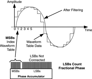
You may recall that a waveform playback controller could never generate a period that was not a multiple of the clock period. In a DDS controller, the addition of fractional phase bits allows the period to vary in infinitesimal fractions of a clock cycle (Figure 16.19). In fact, a DDS controller can be tuned in uniform frequency steps that are the clock period divided by 2^N, where N is the number of bits in the phase accumulator. With a 32-bit accumulator, for example, and a 1-GHz clock, frequencies can be tuned in quarter-hertz steps.

Figure 16.19. Fractional samples.

Since the phase accumulator represents the phase of the periodic waveform being synthesized, simply loading the phase accumulator with a specified phase number causes the synthesized phase to jump to a new state. This is handy for phase modulation. Similarly, the phase increment can be varied causing real-time frequency modulation.

It is remarkable that few ARB controllers include this phase accumulator feature. Given that such a simple extension to the address counter has such a large advantage, it is puzzling why one seldom sees it. In fact, I would say that there really is no fundamental difference between a DDS waveform controller and a waveform playback controller. They are distinguished entirely by the extra fractional bits in the address counter and the ability to program a phase increment with fractional bits.

16.10.2.1. Digital Up-Converter

A close relative of the DDS controller is the digital up-converter. In a sense, it is a combination of a straight playback controller and a DDS in a compound stimulus arrangement as discussed in Section 16.7.6, Compound Stimulus. Baseband data (possibly I/Q) in blocks or “tracks” are played back and modulated on a carrier frequency provided by the DDS.

16.10.3. Algorithmic Sequencing

A basic waveform playback controller has sequencing capabilities when it can play tracks in a programmed order or in loops with repeat counts. The DDS controller adds the ability to perform fractional increments through the waveform, but otherwise has no additional programmability or algorithmic support.

Both the basic waveform playback controller and the DDS controller have only rudimentary algorithmic features and functions, but it is easy to see how more algorithmic features would be useful.

For example, it would be handy to be able to loop and through tracks with repeat counts or to construct subroutines that comprise certain collections of track sequences (playlists in the verbiage of CD players). Not that we want to turn the instrument into an MP3 player, but playlist capability also can assemble message waveforms on the fly based on a signal alphabet. A stimulus with modulated digital data that is provided live, in real time can be assembled from a “playlist.”

It would also be useful to be able to parameterize playlists so that their contents could be varied based on certain conditions. This leads to the requirement for conditional branching, either on external trigger or gate conditions, or on internal conditions—conditions based on the data or on the sequence itself.

As more features are added in this direction, a critical threshold is reached. Instruction memory appears, and along with it, a way for data and program to intermix. The watershed is a conditional branch that can choose one of two sequences based on some location in memory, combined with the ability to write memory. At this point, the controller is a true Turing machine—a real computer. It can now make calculations. Those calculations can either be about data (for example, delays, loops, patterns, alphabets) or they can be generating the data itself (for example, oscillators, filters, pulses, codes).

There is a vast collection of possibilities here. Moving from simple state machines, adding more algorithmic features, adding an algorithmic logic unit (ALU), along with state sequencer capable of conditional branches and recursive subroutines, the controller becomes a dual-memory Harvard-architecture DSP-style processor. Or it may move in a slightly different direction to the general-purpose single-memory Von Neumann processors. Or, perhaps, the controller might incorporate symmetric multiprocessing or systolic arrays. Or something beyond even that.

Obviously, it is also beyond the scope of this book to discuss all the possibilities encompassed in the field of computer architecture. There are many fine books (such as Hennessy, Patterson, and Goldberg, 2002) that give a comprehensive treatment of this large topic. I will, however, make a few comments that are particularly relevant to the synthetic instrumentation application.

16.10.4. Synthesis Controller Considerations

At first glance, a designer thinking about what controller to use for a synthetic instrument application might see the controller architecture choice as a speed/complexity trade-off. On one hand, he or she can use a complex general-purpose processor with moderate speed; and on the other hand, he or she can use a lean-and-mean state sequencer to get maximum speed. Which to pick?

Fortunately, advances in programmable logic are softening this dilemma. As of this writing, gate arrays can implement signal processing with nearly the general computational horsepower of the best DSP microprocessors, without giving up the task-specific horsepower that can be achieved with a lean-and-mean state sequencer. I would expect this gap to narrow into insignificance over the next few years: “Microprocessors are in everything from personal computers to washing machines, from digital cameras to toasters. But it is this very ubiquity that has made us forget that microprocessors, no matter how powerful, are inefficient compared with chips designed to do a specific thing” (Tredennick and Shimamoto, 2003).

Given this trend, perhaps the true dilemma is not in hardware at all. Rather, it might be a question of software architecture and operating system. Does the designer choose a standard microprocessor (or DSP processor) architecture to reap the benefits of a mainstream operating system like vxWorks, Linux, pSOS, BSD, or Windows? Or does the designer roll his or her own hardware architecture specially optimized for the synthetic instrument application at the cost of also needing to roll his or her own software architecture, at least to some extent?

Again, this gap is narrowing, so the dilemma may not be an issue. Standard processor instruction sets can be implemented in gate arrays, allowing them to run mainstream operating systems, and there is growing support for customized ASIC/PLD-based real-time processing in modern operating systems.

In fact, because of advances in gate array and operating system technology, the world may soon see true, general-purpose digital systems that do not compromise speed for complexity and do not compromise software support for hardware customization. This trend bodes well for synthetic instrumentation, which shines the brightest when it can be implemented on a single, generalized CCC cascade.

Extensive computational requirements lead to a general-purpose DSP- or microprocessor-based approach. In contrast, complex periodic waveforms may be best controlled with a high-speed state sequencer implementing a DDS phase accumulator indexing a waveform buffer. While fine resolution-delayed pulse requirements are often best met with hybrid analog/digital pulse generator circuits, these categories intertwine when considering implementation.

16.11. Stimulus Triggering

I have only scratched the surface of the vast body of issues associated with stimulus DSP. One could write a whole book on nothing but stimulus signal synthesis. But my admittedly abbreviated treatment of the topic would be embarrassingly lacking without at least some comment on the issue of triggering.

Probably the biggest topic not yet discussed is the issue of triggering. Triggering is required by many kinds of instruments. How do we synchronize the stimulus and subsequent measurement with external events?

Triggering ties together stimulus and response, much in the same way as calibration does. A stimulus that is triggered requires a response measurement capability in order to measure the trigger signal input. Therefore, an SMS with complete stimulus response closure will provide a mechanism for response (or ordinate) conditions to initiate stimulus events.

Desirable triggering conditions can be as diverse as ingenuity allows. They do not have to be limited to a signal threshold. Rather, trigger conditions can span the gamut from the rudimentary single-shot and free-run conditions to complex trigger programs that require several events to transpire in a particular pattern before the ultimate trigger event is initiated.

16.11.1. Stimulus Trigger Interpolation

Generality in triggering requires a programmable state machine controller of some kind. Furthermore, it is often desirable to implement finely quantized (near continuously adjustable) delays after triggering, which seems to lead us to a hybrid of digital and analog delay generation in the controller.

While programmable analog delays can be made to work and meet requirements for fine trigger delay control, it is a mistake to jump to this hardware-oriented solution. It is a mistake, in general, to consider only hardware as a solution for requirements in synthetic measurement systems. Introducing analog delays into the stimulus controller for the purpose of allowing finely controlled trigger delay is just one way to meet the requirement. There are other approaches.

For example, as shown in Figure 16.20, based on foreknowledge of the reconstruction filtering in the signal conditioner, it is possible to alter the samples being sent to the D/A in such a way that the phase of the synthesized waveform is controlled with fine precision—finer than the sample interval.

Figure 16.20. Fine trigger delay control.

The dual of this stimulus trigger interpolation and resampling technique will reappear in the response side in the concept of a trigger-time interpolator used to resample the response waveform based on the precisely known time of the trigger.

16.12. The Stimulus D/A

The D/A conversion section, or stimulus side codec (or really just “co”), creates an analog waveform based on the output of the digital control section. As I will discuss, the place where the D/A begins and the controller ends may be fuzzy.

D/A converters tend to be constrained by a speed versus accuracy trade-off much in the same way that controllers trade speed for complexity. This speed/accuracy trade-off reflects the practical reality that fast D/A systems tend to have worse amplitude accuracy than slow D/A systems. I am using the word accuracy in the qualitative sense of finer amplitude resolution, measured in bits, but this may also be measured in SiNaD or IMD performance. Speed can be viewed as sampling rate or, equivalently, time resolution. It is most practical to use low-speed D/A subsystems where amplitude accuracy is the primary requirement and to use moderate-amplitude accuracy systems where speed is paramount.

Table 16.2 illustrates typical extremes of this spectrum of trade-offs. It illustrates the typical bandwidth versus accuracy trade-off that one encounters. This does not reflect an exhaustive survey of available D/A technology nor could any static table on a printed page keep up with the fast pace of change.

Table 16.2. D/A converter trade-off range

Requirement	ENOB	Speed
Pulse generation	1-bit	100 GHz
Analog waveforms	12-bit	100 MHz
AC/DC reference	18-bit	100 kHz

Note that ENOB refers to the effective number of bits provided by the amplitude accuracy of a D/A in the given category.

16.12.1. Interpolation and Digital Up-Converters in the Codec

One of the signal coding operations an SMS can be asked to perform is modulation on a carrier, resulting in a so-called bandpass signal. On the stimulus side of a synthetic instrument, there are two fundamental ways to generate a bandpass signal:

• Up-convert digitally before the D/A
• Up-convert with analog circuits after the D/A

It is also possible to do both of these, up-converting to a fixed digital IF before the D/A, and then use analog up-conversion after the D/A to finish the job.

The idea of interpolation in the context of digital signal processing is different than what I mean by interpolation in the context of measurement maps. In DSP terms, interpolation is a process of increasing the sampling rate of a digital signal. It is accomplished by means of an interpolating filter that reconstructs the missing samples with predicted data based on the assumption of a limited signal bandwidth. A good reference on the interpolation process is Vaidyanathan (1993). Interpolation goes hand-in-hand with up-conversion since a higher-frequency up-converted result needs more samples to represent it without aliasing.

You may be puzzled why up-conversion and interpolation is a topic for the stimulus codec section of this book. Is digital up-conversion not accomplished by the stimulus controller? Is analog up-conversion not a signal conditioning function? Yes, I agree that logically the up-conversion function is not part of the codec, but the fact is that many new D/A subsystems are being built with digital up-conversion and interpolation on board.

Actually, it is quite beneficial for interpolation and digital up-conversion to be accomplished within the stimulus codec. This is good because it lowers the data rate required out of the stimulus controller. In a sense, the stimulus controller can concern itself only with the meaningful portion of the stimulus. The resulting baseband or low-IF signal can then be translated in a mechanical process to some high frequency without burdening the controller. In a sense, the codec is merely coding the information bearing portion of the signal, both as an analog voltage and as a modulation.

The idea of accomplishing signal encoding in the D/A subsystem extends beyond just up-conversion and analog coding. Other forms of encoding can be accomplished most efficiently here. These possibilities include pulse modulation, AM/FM modulation, television signals such as NTSC/ PAL, frequency hopping, and direct sequence spreading.

In general, never assume that all DSP tasks are performed in the stimulus controller; never assume all analog conditioning tasks are performed in the stimulus conditioner. All the hardware is available to be used for anything.

16.13. Stimulus Conditioning

In a stimulus system, after the analog signal is synthesized by the D/A, some amount of signal conditioning may need to be applied. This conditioning can include a wide variety of signal processing and DUT-specific considerations including, possibly, one or more of the following:

• Amplification: linear, digital, pulse, RF, high voltage, or current
• Filtering: fixed, tunable, tracking, adaptive
• Impedance: matched source, programmable mismatch, constant current/voltage
• DUT interface: probes, connectors, transducers, antennas

DUT interfacing is the normal role for signal conditioning; however, as I just explained with regard to the D/A, there is no reason that signal encoding or modulation tasks cannot be performed here as well, especially up-conversion and modulation. An analog RF up-converter is a common signal conditioner component.

Signal-conditioning requirements are obviously dependent on the needs of the DUT, but they are also dependent on the performance of the D/A subsystem. If, for example, the D/A is fast enough to generate all frequencies of interest, there is no need for up-conversion; if the D/A can produce the required power, current, or voltage, there is no need for amplification.

The need to interact with a diverse selection of DUTs tends to drive the design of stimulus signal conditioning in the direction of either a parameterized asset, as I discussed in Section 16.7.4, Parameterization of CCC Assets, or to multiple assets in the CRM architecture sense. Often parameterization makes the most sense as it is more efficient to contain the switching between different conditioner circuit options within some overall conditioner subsystem than it is to force the system-level switching to handle this. Only when faced with a unique and narrow range of conditioning needs specific to a certain class of DUTs does it make sense to create a unique conditioner asset to address that requirement.

An illustration of this principle would be a variable gain amplifier or selectable filter in the signal conditioner. It would make no sense to build separate conditioners just to change a gain or a filter. Similarly, DC offsets, impedances, and other easily parameterized qualities are best implemented that way.

The opposite case would be a situation where the signal conditioner could produce a signal that would be damaging to some class of assets or where some class of DUTs could do damage to the conditioner, for instance, a high-voltage stimulus.

16.13.1. Stimulus Conditioner Linearity

Stimulus conditioner circuitry does not have to be linear in all cases. It depends on the requirements of the test. Some applications, pulsed digital test, for instance, might be best served with digital line drivers as the signal conditioner amplifiers. Such drivers are not linear devices.

In other applications, linearity after the D/A is paramount. It is also generally beneficial to minimize the noise and spurious signals added after the D/A.

Problems with stimulus conditioner linearity are exacerbated when the stimulus conditioner is an analog up-converter. It is very difficult to preserve wide dynamic range, limit the injection of noise, and prevent spurious products from appearing at the stimulus output.

Because linear conditioner design can be challenging and expensive, it is important to keep an open mind about solutions to these difficulties.

16.13.2. Gain Control

Although it is definitely most convenient to adjust the level (amplitude) of the stimulus by simply adjusting the amplitude of the digital signal entering the D/A, sometimes this is not a good idea. If the signal conditioner has an up-converter or other gain or spurious producing stages, the junk injected by this conditioner circuitry remains at a constant level as the signal out of the D/A drops (Figure 16.21). The D/A itself may also inject some unwanted signals at a fixed level. Consequently, the signal-to-noise ratio (SNR) of the stimulus will fall as the stimulus level is decreased relative to the fixed noise. In fact, the fixed noise-level may limit the minimum stimulus signal that is discernible, as eventually noise will swamp the signal.

Figure 16.21. Effect of gain control placement on SNR with varying gain.

The way around this problem is to adjust signal levels in the stimulus conditioner after most of the junk has been added to the signal. That way, when adjusting the signal level, the SNR stays roughly the same. The signal level can be lowered without fear that it will be swamped by the noise.

As a result of this idea, stimulus signal conditioners are often designed with variable-gain amplifiers or adjustable output attenuation. This allows us to run the D/A at an optimum signal level relative to headroom and quantization noise.

Adjusting gain in the signal conditioner is not without its disadvantages. Foremost of these is that the variable gain must be implemented so as to work and maintain calibration across the range of frequencies and signals that the conditioner might handle. This can be a challenge in broadband designs. Sometimes a compromise approach is used, with only coarse gain steps (perhaps 10 dB) implemented in the conditioner, with fine steps implemented in the codec or DSP controller.

16.13.3. Adaptive Fidelity Improvement

Often, the designers of synthetic measurement systems struggle to achieve impeccable fidelity in the stimulus signal conditioning so as to preserve all the precision in the stimulus they have generated with the finely quantized D/A. Building a “clean” enough signal conditioner good enough to match the D/A is often a daunting challenge. It is particularly difficult to meet fidelity specifications in generic hardware when they derive from a the performance of a signal-specific instrument. I have seen stimulus system designers struggle with this again and again. Designing up-converters with high fidelity and low spurs is additionally difficult.

Granted, it is harder to make a clean sine wave with a D/A and broadband analog processing than it is with a narrow-band filtered crystal oscillator, but this may be an unnecessary enterprise. As I will say repeatedly in this book, proper synthetic instrument design focuses on the measurement, not on the specifications of some legacy instrument being replaced. Turn to the measurement to see what fidelity is needed. You may find that much less is needed by the measurement than what a blanket fidelity specification would require.

Once we have focused on the measurement and looked at the fidelity performance of reasonable stimulus signal conditioning, if we see that we still do not meet the requirements for a good measurement, what do we do then? Clearly, the solution to that underspecified problem depends on the details of the situation. In some cases, parameterized filtering would help, other times higher-power amplification can improve linearity. These are all well-known techniques. But there is one technique I want to mention here because it is often overlooked—a technique that has wide applicability to these situations: adaptive processing.

Remember, there is a response system at our disposal, and a fully programmable, DSP-driven stimulus system to boot. This combination lends itself nicely to closed-loop adaptive techniques.

If you can measure and you can control, then you can adapt to achieve a measured goal. Specifically, it is possible to adapt the digital data driving the D/A so as to reduce or eliminate artifacts, spurs, and other fidelity issues introduced by the signal conditioner.

A simple example of this technique would be the elimination of a spurious tone that appears in the stimulus output that is harmful to a measurement. Synthesize a second tone of the same frequency as the spur. Figure 16.22 shows a system for adaptively adjusting the amplitude and phase of the second tone to null the spur, eliminating it from the stimulus and thus making the measurement possible.

Figure 16.22. Adaptive nulling.

Adaptive nulling, linearization, or calibration is a nontrivial enterprise to be sure, but it has the unique property in this context of being something that can be implemented purely in DSP software. That does not mean it is necessarily easier or better than a hardware solution to a fidelity issue. My point, however, is that such techniques should always be considered when the hardware has fidelity issues. Adaptive DSP techniques will often have a significantly lower cost in production than any hardware solution.

16.13.4. Reconstruction Filtering

Depending on the needs of the test, it may be possible to directly use the quantized voltage from the output of the stimulus codec. For example, if the stimulus is a digital logic level, it may be used directly. However, when synthesizing a smooth analog stimulus waveform, it is often better to use a reconstruction or interpolation filter. This filtering at the output of the D/A reconstructs the analog waveform from the “stair-step” approximation. Spectrally, this filter attenuates high-frequency aliases while it can also correct for the sin(x)/x roll-off effect created by holding the samples through each “tread” in the staircase.

If I know the dynamics of the reconstruction filtering when I am calculating the samples I will send into the stimulus codec, it is possible for me to choose these samples to custom tailor and shape in the signal conditioner output waveform based on that knowledge.

For example, fine control of rise time and delay is possible using this technique—10 times finer than the sample interval, even. This is a critical fact to keep in mind when designing the codec. It is easy to see a specification that says “rise time programmable in 1-nS steps” and erroneously conclude that the D/A must run at 1 GHz.

The characteristics of the reconstruction filtering and other fixed or parameterized filters in the signal conditioner can also be used to facilitate adaptive techniques, as described in Section 16.13.3, Adaptive Fidelity Improvement.

16.14. Stimulus Cascade—Real-World Example

Figure 16.23 shows an example of a real-world stimulus subsystem, the Celerity Series CS25000 broadband signal and environment generator (BSG), from Aeroflex. This is only one of the many different stimulus products made by Aeroflex. I selected this one in particular because it includes both high-fidelity signal conditioning and stimulus processing that comprises both a waveform playback controller and general-purpose CPU with a range of options. Thus, the Aeroflex broadband signal and environment generator platform represents a complete synthetic measurement system stimulus cascade.

Figure 16.23. Aeroflex CS25000.

The BSG combines a very deep memory, very high-speed arbitrary waveform generator, and a broadband RF up-converter with powerful signal generation software. The BSGs have bandwidths of up to 500 MHz and full-bandwidth signal memory of up to 10 s. The bandwidth, memory depth, and dynamic range make the BSG a powerful tool for broadband satellite communications, frequency agile radio communications, broadband wireless network communications, and radar test (Table 16.3). An open, software-defined instrument architecture allows easy imports of user-created waveforms. Vector signal simulator (VSS) software creates signal files for commercial wireless standards as well as generic nPSK, nQAM, nFSK, MSK, CW, tone combs, and notched noise signals.

Table 16.3. BSG performance range

Model number	Bandwidth	Sample rates	Sample size	Dynamic range	Max memory
CS25020	75 MHz	200 MS/s	14 bits	70 dB	2048 MS
CS25025	200 MHz	250 MS/s	12 bits	60 dB	2048 MS
CS25040	160 MHz	400 MS/s	8 bits	45 dB	4096 MS
CS25080	280 MHz	700 MS/s	8 bits	45 dB	8192 MS
CS25082	280 MHz	700 MS/s	12 bits	55 dB	8192 MS
CS25130	500 MHz	1300 MS/s	8 bits	45 dB	16384 MS
CS25132	500 MHz	1300 MS/s	12 bits	55 dB	16384 MS

Any of these generic signal types can be gated or bursted in time, as well as hopped in frequency. Real signals, including recorded signals from Aeroflex's broadband signal analyzers or other recorder sources, can be imported and combined with digitally generated signals and then played back on the BSG (Table 16.4). Impairments can be added to the signals including thermal noise, phase noise, and passband amplitude and phase distortion. VSS provides the unique ability to mix any combination of signals and impairments to generate complex signal environments.

Table 16.4. BSG options

Frequency down-converter option	Tunable or fixed up to 40 GHz in bands
Memory sequencing option	High-speed address sequencing
Output options	Precision attenuators
High-speed attenuators
Reconstruction filters
Sample clock option	Low phase noise
Disk storage options	Fixed and removable drives
73 GB to 146 GB
CD-RW, CD-ROM, DVD
Multiple signal options	IF/RF
Baseband	Digital
Controller options	UltraSPARC/Solaris
Remote control options	Pentium/Linux
10/100Base-T Ethernet
GPIB
Peripheral options	Keyboard and mouse
Flat panel and CRT monitors
Playback/output options	Wide-band analog
High-speed digital (LVDS, DECL, PECL, TTL)

Aeroflex's Vector signal player (VSP) software provides simple controls for signal file selection, output frequency control, and output power control. Aeroflex's up-converters use real (non-I/Q) conversion architectures, generating high dynamic range waveforms without the carrier leakage and signal image problems associated with I/Q modulators found in other signal sources.

The high-speed stimulus controller in the BSG is designed with an enhanced version of the waveform playback architecture I discussed in Section 16.10.1, Waveform Playback. This controller allows the BSG to play extremely complicated waveform data files through the use of programmed sequencing. This allows for the predetermined, scenario-based playback of different sections in memory. During playback, the instrument can move from one section of memory to another, on a clock cycle. The control of this is analogous to a typical MIDI tone generator driven by a sequencer (a high-tech player piano). The BSG waveform address counter can move in programmed fashion to different sections of memory, building a complete stimulus output without having to put the complete wave train into memory.

This sequencing capability is particularly useful when synthesizing digital modulation waveforms. It makes efficient use of memory while allowing many possible waveforms to be generated. A simple example would be a pulse that is only active for a small amount of time. The pulse can be put into a small block of memory, another small block of memory can hold a piece of interpulse signal (often just zeros). A scenario file programs the system to play the interpulse buffer for a certain number of cycles, then to play the pulse file once, then to start over. There can be multiple pulse profiles and interpulse buffer profiles that can be played to produce extremely complex output stimulus from a small amount of memory.

16.15. Real-World Design: A Synthetic Measurement System

So far, I have talked rather philosophically about synthetic measurement system design issues. The examples I have given and detailed techniques I have discussed have all been abstract, not referring to any particular measurement system or instrument implementation. The following sections are different. Here, I present a real-world synthetic measurement system that is in operation today (2004). Sections 16.15 through 16.21 are courtesy of the Raytheon and Aeroflex Companies and are based on an Auto Test Con paper (Hatch, Brandeberry, and Knox, 2003) that describes a high-speed, high-performance RF test system targeted for a moderate- to high-quantity manufacturing environment.

16.16. Universal High-Speed RF Microwave Test System

The real-world system I will discuss in the following sections was developed by Raytheon. The RF multifunction test system (RFMTS) was developed to provide for a wide variety of RF test demands and targeted at radically reducing test times. It is a versatile test system integrating state-of-the-art capabilities in high-speed RF testing, microwave synthetic instrument measurement techniques, product interfacing, and calibrating.

16.16.1. Background

Trends in military product design have been toward modular, solid-state RF microwave architectures, taking advantage of major improvements in solid-state RF component design. For example, radar architectures are now based on using thousands of solid-state modules packaged in manageable assemblies of up to 30 modules each. This shift in design architecture has precipitated demand for a flexible high-speed, high-quality RF microwave test system.

In 1999, Raytheon embarked on a venture of developing such a system. Besides high throughput and versatility, the goals of the project included logistic goals that would address lowering life-cycle costs, technical goals that would achieve high performance, and an architecture that would enable it to maintain technical excellence.

16.16.2. Logistical Goals

The main focus was to develop a system that would permit lowering life-cycle costs. The goal translated into a common platform that could be used in a broad spectrum of applications. If achieved this would enable

• Training for one system versus many for operators, maintainers, and TPS developers
• Reduced calibration equipment and procedures
• System self-test to permit increased availability
• A modular architecture to facilitate maintenance, require fewer spares, and deal with obsolescence
• A spares and maintenance program for one system
• A common resource that could be shared across many programs
• An open architecture (hardware and software) that would promote system longevity and permit upgrading

16.16.3. Technical Goals

Architecture was a major consideration at the core of the technical goals. The objective was to have a modular system based on industry standards from both a hardware and software viewpoint and minimize dependence upon proprietary designs.

16.16.4. RF Capabilities

The first criterion was measurement speed. Experience with heretofore “high-speed” test systems achieved test times of approximately a half hour for solid-state assemblies. Classical rack-and-stack RF test systems needed hours to test complex receiver/exciter assemblies. Goals were to reduce these times by factors from 3 to 10.

Nearly as important as speed was RF measurement performance. A fast system with marginal performance would not have a wide range of applications. This new system had to have measurement performance capability similar to that of typical commercial test instrumentation. For it to be able to do the job, the system needed to have an extensive measurement suite. In the RF world, where cable losses and other transmission line issues can be serious problems, an instrument with good measurement capability at its front panel is only half the solution. Being able to easily extend the measurement all the way to the DUT was a prime consideration. Hence, having flexible calibration options was high on the list of priorities.

16.17. System Architecture

The blend of a synthetic measurement system (the Aeroflex TRM1000C) and a Raytheon custom-designed third bay (RF switch matrix, DUT interface assembly, and auxiliary COTS equipment) provided a solution that met the desired hardware goals. The software goals were achieved by taking advantage of the TRM1000C industry standard LabWindows/CVI, VXI plug-and-play-type drivers, and LabWindows/CVI-compatible GPIB instrumentation in the Raytheon-designed third bay.

16.17.1. Microwave Synthetic Instrument (TRM1000C)

The Aeroflex TRM1000C is designed to provide reconfigurable, high-speed production test equipment for evaluating a variety of different microwave devices such as amplifiers, transmit and receive (T/R) modules, frequency translation devices, receivers, local oscillators, and phase shifters. It can also perform tests on integrated subassemblies of RF components, as well as on full up-systems filled with any combination of active RF, multiport devices.

The basic architecture of the TRM1000C is consistent with the basic architecture described in this chapter, a CCC cascade, enhanced with compound signal conditioners. The compound conditioners consist of a stimulus up-converter and a response down-converter. Time multiplexing is used to expand the system to multiple inputs and outputs. A calibration and verification system allows for loopback ordinates and application of metrology standards. Figure 16.24 outlines this high-level functionality.

Figure 16.24. TRM1000C functional diagram.

The TRM1000C is designed to dramatically improve module test times and reduce measurement errors introduced by the operator, test hardware, and DUT interface. It is ideally suited for production test applications where throughput and flexibility are paramount. Through its synthetic design, the TRM1000C's nonspecific RF hardware can be software configured to run specific RF and microwave production tests. The TRM1000C hardware architecture is based on advanced synthetic instrument concepts; the TRM1000C does the same measurements as several distinct microwave test instruments including a pulsed power meter, a frequency counter, multiple sources, a spectrum analyzer, a vector network analyzer, a noise figure meter, and a pattern generator. The full measurement suite is as in Table 16.5.

Table 16.5. TRM1000C measurement suite

Power	RF signal source
Tone power	Complex volts
Pulse power (rms or peak)	Pulse profile
Total power	Rise time
Spectral POWER Density	Fall time
Noise power	Droop
Pout and pin at N dB compression	Envelope delay
AM/PM	Frequency
Multiport S-parameters	Spurii
12-Term error correction	Harmonic
Gain	Nth ORDER Intercept
Input/output return loss	Modulation index
Isolation	Raw read
Conversion gain	Complex FFT data block
Group delay	Digital data verification
Noise figure	Analog DMM
Phase noise	Scope measurements

A standard TRM1000C includes complex stimulus generation including pulsed modulation, AM, FM, phase modulation (PM), and a fast response measurement channel. Since the system is synthetic in design and thereby easily reconfigurable, the system can be reused for different programs and applications, therefore maximizing return on investment (ROI).

If you look carefully at the block diagram in Figure 16.24, you can see that the internal design of the TRM1000C follows the standard synthetic measurement system CCC architecture principles for both stimulus and response. A compound up-converter in the stimulus and a compound down-converter in the response side orients the TRM1000C architecture toward the generation and analysis of bandpass signals, as is appropriate to its RF measurement mission. A calibration matrix interconnects stimulus and response with the DUT, providing stimulus/response closure. This eliminates many redundancies (for example, duplicated channels, stimulus-side detectors, response-side sources) that would otherwise be necessary in order to maintain calibration.

16.17.2. Supplemental Resources

Practical design realities limited the scope of what could be achieved with a purely synthetic measurement system. For testing the more complex RF products (receiver/exciter elements, frequency translation devices, and so forth), additional nonsynthetic resources were required. These instruments do not need to be inside the high-speed loops of the synthetic instrument and therefore do not interfere with measurement speeds. The supplemental test instrument resources include three RF sources, an oscilloscope, digital multimeter (DMM), and power meter (for troubleshooting purposes). These instruments, the RF switch matrix, and DUT interface were incorporated into Raytheon-designed third bay to complement the TRM1000C.

16.18. DUT Interface

For the RFMTS to easily work with a variety of RF products, some way to interface its test resources to these products had to be developed. The interface needed to be rugged, versatile, high performance, and easy to use. In addition, a high-performance RF switch matrix was included as part of this assembly in order to permit simple, low-cost interface adapters. The chosen solution integrates a high-performance RF switch matrix and a Virginia Panel interface assembly as shown in Figure 16.25.

Figure 16.25. Test adapter interface.

16.18.1. Product Test Adapter Solutions

Some of the products to be tested on the RFMTS were known to be large assemblies. For this reason, time was spent on developing calibration schemes that could be extended out several levels and on providing a rugged, high-performance interface. This approach has permitted using the system on virtually any size RF product. It also accommodates other relatively unique items that support the test, such as pneumatics, hydraulics, and liquid cooling.

16.19. Calibration

The RFMTS is designed to collect measurement data for a variety of different DUTs. By the nature of the measurement, raw data collected by the instrument contains characteristics of both the DUT and the test system hardware (instrument, switch interface, DUT adapter, and so forth). To extract only the characteristics of the DUT, the system must compensate for its own contribution to the measurement data. The process for characterizing the system's contribution is generically termed calibration.

Calibration is an integral part of performing measurements. Calibration procedures are dependent on the application, measurement, and measurement method; therefore, the flexible TRM1000C calibration design allows for different applications needs. The measurements must be NIST traceable; therefore, NIST-traceable transfer standards are needed to calibrate the system.

TRM1000C calibration is divided into two categories: primary calibration and operational calibration.

16.19.1. Primary Calibration

The TRM1000C utilizes the modular, line-replaceable-unit (LRU) methodology as part of the system. These LRUs are calibrated at a standard metrology calibration lab and become an integral part of the system. The majority of the LRUs are commercially available NIST-traceable standards. The production floor can have spares available to remove and replace, minimizing system downtime when performing periodic maintenance. The LRUs also eliminate the need for external, on-site support equipment; therefore, the user does not need to bring external equipment up to the system.

A list of primary calibrated LRUs is as follows:

• Power meter (50-MHz source)
• Power sensor calibration factor
• Noise source excess noise ratio (ENR)
• 10-MHz rubidium standard
• 3.5-mm calibration kit (S-parameters)

16.19.2. Operational Calibration

This is an application-specific procedure that transfers the measurement standards from the system's calibration LRUs to the system itself. This calibration can handle a number of different multiport devices and any number of DUT interfaces. The DUT interfaces can be as simple as NIST-traceable coaxial connectors (3.5 mm), or the interface can be more complex: non-NIST-traceable coaxial connectors (for example, GPPO), standard and nonstandard waveguide, or even direct wafer probes. A multitier calibration technique is used to extend the calibration reference plane out to the DUT (deembed).

16.20. Software Solutions

With a synthetic instrument approach, the scope and potential capabilities of the software are almost boundless. The entire system is LabWindows/CVI-based. A software architecture has been used to address a variety of goals and desired capabilities:

1. Ease of use by TPS developers and test system maintainers
2. Sufficient depth and flexibility to accommodate dealing with very complex, digitally controlled RF products
3. The different levels of software employed by the TRM1000C synthetic instrument

16.20.1. Test Program Set Developer Interface

The objective here was to provide a simplistic means of implementing moderately complex tests, without demanding that all test program set (TPS) developers/maintainers be experts in C programming. The solution was to develop C-based test procedures that would be graphical in nature and then utilize a test executive that would readily permit stringing these test procedures together. This approach requires a few C experts but permits test engineers to be productive with minimal software specific training.

The test procedure concept simply translates typical RF measurement scenarios in a graphical user interface screen or “panel” where the required parameters can be entered. The TPS designer enters the associated parameters via the panel for each test the designer develops. Test procedures have been developed for all of the measurement types.

A primary objective of the test procedure approach is to maximize reuse and provide cost-effective TPSs in a timely manner. The approach has proven to be very effective. Test engineers are able to concentrate on the technical aspects of the DUT and the test scenarios. The pure software designers are doing what they do best—developing the C-based procedures in support of the test designers. In the event of complex tests, the LabWindows/CVI environment provides a very flexible environment for developing custom procedures for unique or even further speed enhancement if required.

16.20.2. TRM1000C Software

The TRM1000C currently uses a scripting language called JavaScript (ECMAScript). Scripts are used to define the logic, control, processing, and storage of the measurement and resultant data. Any number of scripts may be loaded at any time and sequenced via a test executive or incorporated as part of a test procedure and then called by an executive. Through commanding of the scripts, the TRM1000C may change from one measurement personality (i.e., vector network analysis) to another (noise figure).

There are two categories of scripts that can be designed: low level and high level. Low-level scripts are interpreted and run one step at a time. A low-level script is not optimized for speed but is best for situations where the number of firmware states is unknown. Such a situation may arise when conditional branching is utilized. An example of this is when a measurement result is used to decide whether another measurement needs to be made.

High-level scripts are unrolled and loaded into a state table within the processor. The processor can then execute the state table without any interaction with the script. This method is optimized for speed, but requires a known number of states.

After the measurement is performed, the requested data is stored in a local data file (slot zero controller). Since the scripting capability allows for complex, multidimensional data sets to be collected and the speed of the system allows for considerable data to be collected quickly, these data files can be somewhat large. To minimize the data file size and to allow for easy access, the TRM1000C currently utilizes an open file format called hierarchical data format (HDF). Measurement results can then be either routed back through the host driver link as part of the script or the HDF file can be retrieved remotely by the host. Any number of different test executives can be used with the TRM1000C. Test executive software running on the host PC performs all data presentation and report generation activities.

16.21. Conclusions

The system performance is comparable to that of stand-alone instrumentation and in some cases better. From a practical application viewpoint, the RFMTS performance has met all required DUT test requirements, many of which are very stringent.

Relative to use of the term typical, it is very important to note that the test designer has a great deal of leeway relative to optimizing measurement and speed performance. The test designer has control over the IF bandwidth, DSP block size (number of samples), block count (averages), receiver gain, and so forth, therefore, allowing for optimizing performance for a required measurement. From practical experience, there are DUTs tested on the system that are optimized for speed and others that are optimized for measurement performance. In typical applications, the high-volume devices have measurement requirements that permit optimizing for speed. The DUTs that require the greatest accuracy are much fewer in number on a per-system basis, and therefore, minor sacrifices of speed are easily accepted.

As a last note relative to performance, the TRM1000C synthetic design and system architecture readily permits performance improvements via both hardware and software, and in fact these improvements are continually being made.

From both a logistical and technical goal viewpoint, the system has been a major success. Multiple systems are on the floor, and the envisioned goals are now being realized. The open architecture, the speed, and the technical performance have made the RFMTS a standard core test system. The architecture permits continual growth from both hardware and software viewpoints.

Hardware growth will focus on continued performance enhancements. With the modular approach, this can and is being done in an incremental fashion. Even speed, one of the system's main virtues continues to improve as computer speeds and the other building blocks in the system improve. But software will be the most exciting area where continual growth is envisioned. The graphical test procedures will continually be refined. They will be made more user-friendly, increased in depth, and more specific elements will be added. As these grow and develop, the cost and schedule for developing test programs will likewise reduce. Because of the nature of the system, software can and will enhance every aspect of the system: performance, utilization, calibration, and maintenance.

References

Carlson 1968 A. Bruce Carlson, Communication Systems 1968 McGraw-Hill New York

Fuller 1975 R. Buckminster Fuller, Synergetics 1975 Macmillan New York

Hatch 2003 Robert. R. Hatch, Brandeberry Randall, Knox William, Universal High Speed RF Microwave Test System 2003 Auto Test Con, Institute of Electrical and Electronics Engineers Anaheim, CA September 2003

Hennessy 2002 John L. Hennessy, David A Patterson, Goldberg David, Computer Architecture: A Quantitative Approach 3rd ed 2002 Morgan Kaufmann San Mateo, CA

Tredennick 2003 Nick Tredennick, Shimamoto Brian, Go Reconfigure IEEE Spectrum 200336-40

Vaidyanathan 1993 P.P. Vaidyanathan, Multirate Systems and Filter Banks 1993 Prentice Hall Englewood Cliffs, NJ