Chapter 15. Scaling and Calibration

The task of a data-acquisition program is to determine values of one or more physical quantities, such as temperature, force, or displacement. This is accomplished by reading digitized representations of those values from an ADC. In order for the user, as well as the various elements of the data-acquisition system, to correctly interpret the readings, the program must convert them into appropriate “real-world” units. This obviously requires a detailed knowledge of the characteristics of the sensors and signal-conditioning circuits used. The relationship between a physical variable to be measured (the measurand) and the corresponding transduced and digitized signal may be described by a response curve such as that shown in Figure 15.1.

Figure 15.1. Response curves for typical measuring systems: (a) linear response and (b) nonlinear response.

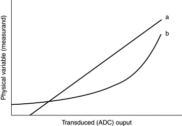
Each component of the measuring system contributes to the shape and slope of the response curve. The transducer itself is, of course, the principal contributor, but the characteristics of the associated signal-conditioning and ADC circuits also have an important part to play in determining the form of the curve.

In some situations the physical variable of interest is not measured directly: It may be inferred from a related measurement instead. We might, for example, measure the level of liquid in a vessel in order to determine its volume. The response curve of the measurement system would, in this case, also include the factors necessary for conversion between level and volume.

Most data-acquisition systems are designed to exhibit linear responses. In these cases either all elements of the measuring system will have linear response curves or they will have been carefully combined so as to cancel out any nonlinearities present in individual components.

Some transducers are inherently nonlinear. Thermocouples and resistance temperature detectors are prime examples, but many other types of sensor exhibit some degree of nonlinearity. Nonlinearities may, occasionally, arise from the way in which the measurement is carried out. If, in the volume-measurement example just mentioned, we have a cylindrical vessel, the quantity of interest (the volume of liquid) would be directly proportional to the level. If, on the other hand, the vessel had a hemispherical shape, there would be a nonlinear relationship between fluid level and volume. In these cases, the data-acquisition software will usually be required to compensate for the geometry of the vessel when converting the ADC reading to the corresponding value of the measurand.

To correctly interpret digitized ADC readings, the data-acquisition software must have access to a set of calibration parameters that describe the response curve of the measuring system. These parameters may exist either as a table of values or as a set of coefficients of an equation that expresses the relationship between the physical variable and the output from the ADC. In order to compile the required calibration parameters, the system must usually sample the ADC output for a variety of known values of the measurand. The resulting calibration reference points can then be used as the basis of one of the scaling or linearization techniques described in this chapter.

15.1. Scaling of Linear Response Curves

The simplest and, fortunately, the most common type of response curve is a straight line. In this case the software need only be programmed with the parameters of the line for it to be able to convert ADC readings to a meaningful physical value. In general, any linear response curve may be represented by the equation (15.1)

where y represents the physical variable to be measured and x is the corresponding digitized (ADC) value. The constant y⁰ is any convenient reference point (usually chosen to be the lower limit of the range of y values to be measured), x⁰ is the value of x at the intersection of the line y = y⁰ with the response curve (i.e., the ADC reading at the lower limit of the measurement range), and s represents the gradient of the response curve.

Many systems are designed to measure over a range from zero up to some predetermined maximum value. In this case, y⁰ can be chosen to be zero. In all instances y⁰ will be a known quantity. The task of calibrating and scaling a linear measurement system is then reduced to determining the scaling factor, s, and offset, x⁰.

15.1.1. The Offset

The offset, x⁰, can arise in a variety of ways. One of the most common is due to drifts occurring in the signal-conditioning circuits as a result of variations in ambient temperature. There are many other sources of offset in a typical measuring system. For example, small errors in positioning the body of a displacement transducer in a gauging jig will shift the response curve and introduce a degree of offset. Similarly, a poorly mounted load cell might suffer transverse stresses which will also distort the response curve.

As a general rule, x⁰ should normally be determined each time the measuring system is calibrated. This can be accomplished by reading the ADC while a known input is applied to the transducer. If the offset is within acceptable limits it can simply be subtracted from subsequent ADC readings as shown by Equation (15.1). Very large offsets are likely to compromise the performance of the measuring system (e.g., limit its measuring range) and might indicate faults such as an incorrectly mounted transducer or maladjusted signal-conditioning circuits. It is wise to design data-acquisition software so that it checks for this eventuality and warns the operator if an unacceptably large offset is detected.

Some signal-conditioning circuits provide facilities for manual offset adjustment. Others allow most or all of the physical offset to be cancelled under software control. In the latter type of system the offset might be adjusted (or compensated for) by means of the output from a digital-to-analog converter (DAC). The DAC voltage might, for example, be applied to the output from a strain-gauge-bridge device (e.g., a load cell) in order to cancel any imbalances present in the circuit.

15.1.2. Scaling from Known Sensitivities

If the characteristics of every component of the measuring system are accurately known, it might be possible to calculate the values of s and x⁰ from the system design parameters. In this case the task of calibrating the system is almost trivial. The data-acquisition software (or calibration program) must first establish the value of the ADC offset, x⁰, as described in the preceding section, and then determine the scaling factor, s. The scaling factor can be supplied by the user via the keyboard or data file, but, in some cases, it is simpler for the software to calculate s from a set of measuring-system parameters typed in by the operator.

An example of this method is the calibration of strain-gauge-bridge transducers such as load cells. The operator might enter the design sensitivity of the load cell (in millivolts output per volt input at full scale), the excitation voltage supplied to the input of the bridge, and the full-scale measurement range of the sensor. From these parameters the calibration program can determine the voltage that would be output from the bridge at full scale, and knowing the characteristics of the signal-conditioning and ADC circuits, it can calculate the scaling factor.

In some instances it may not be possible for the gain (and other operating parameters) of the signal-conditioning amplifier(s) to be determined precisely. It is then necessary for the software to take an ADC reading while the transducer is made to generate a known output signal. The obvious (and usually most accurate) method of doing this is to apply a fixed input to the transducer (e.g., force in the case of a load cell). This method, referred to as prime calibration, is the subject of the following section. Another way of creating a known transducer output is to disturb the operation of the transducer itself in some way. This technique is adopted widely in devices, such as load cells, that incorporate a number of resistive strain gauges connected in a Wheatstone bridge. A shunt resistor can be connected in parallel with one arm of the bridge in order to temporarily unbalance the circuit and simulate an applied load. This allows the sensitivity of the bridge (change in output voltage divided by the change in “gauge” resistance) to be determined, and then the ADC output at this simulated load can be measured in order to calculate the scaling factor. In this way the scaling factor will encompass the gain of the signal-conditioning circuit as well as the conversion characteristics of the ADC and the sensitivity of the bridge itself.

This calibration technique can be useful in situations, as might arise with load measurement, where it is difficult to generate precisely known transducer inputs. However, it does not take account of factors, resulting from installation and environmental conditions, which might affect the characteristics of the measuring system. In the presence of such influences this method can lead to serious calibration errors.

To illustrate this point we will continue with the example of load cells. The strain gauges used within these devices have quite small resistances (typically less than 350Ω). Consequently, the resistance of the leads that carry the excitation supply can result in a significant voltage drop across the bridge and a proportional lowering of the output voltage. Some signal-conditioning circuits are designed to compensate for these voltage drops, but without this facility it can be difficult to determine the magnitude of the loss. If not corrected for, the voltage drop can introduce significant errors into the calibration.

In order to account for every factor that contributes to the response of the measurement system, it is usually necessary to calibrate the whole system against some independent reference. These methods are described in the following sections.

15.1.3. Two- and Three-Point Prime Calibration

Prime calibration involves measuring the input, y, to a transducer (e.g., load, displacement, or temperature) using an independent calibration reference and then determining the resulting output, x, from the ADC. Two (or sometimes three) points are obtained in order to calculate the parameters of the calibration line. In this way the calibration takes account of the behavior of the measuring system as a whole, including factors such as signal losses in long cables.

By determining the offset value, x⁰, we can establish one point on the response curve—that is, (x⁰, y⁰). It is necessary to obtain at least one further reference point, (x¹, y¹), in order to uniquely define the straight-line response curve. The scaling factor may then be calculated from (15.2)

Some systems, particularly those that incorporate bipolar transducers (i.e., those that measure either side of some zero level), do not use the offset point (x⁰, y⁰) for calculating s. Instead, they obtain a reading on each side of the zero point and use these values to compute the scaling factor. In this case, y⁰ might be chosen to represent the center (zero) value of the transducer's working range and x⁰ would be the corresponding ADC reading.

15.1.4. Accuracy of Prime Calibration

The values of s and x⁰ determined by prime calibration are needed to convert all subsequent ADC readings into the corresponding “real-world” value of the measurand. It is, therefore, of paramount importance that the values of s and x⁰, and the (x⁰, y⁰) and (x¹, y¹) points used to derive them, are accurate.

Setting aside any sampling and digitization errors, there are several potential sources of inaccuracy in the (x, y) calibration points. Random variations in the ADC readings might be introduced by electrical noise or instabilities in the physical variable being measured (e.g., positioning errors in a displacement-measuring system).

Electrical noise can be particularly problematic where low-level transducer signals (and high amplifier gains) are used. This is often the case with thermocouples and strain-gauge bridges, which generate only low-level signals (typically several millivolts). Noise levels should always be minimized at source by the use of appropriate shielding and grounding techniques. Small amplitudes of residual noise may be further reduced by using suitable software filters. A simple 8× averaging filter can often reduce noise levels by a factor of 3 or more, depending, of course, upon the sampling rate and the shape of the noise spectrum.

An accurate prime calibration reference is also essential. Inaccurate reference devices can introduce both systematic and random errors. Systematic errors are those arising from a consistent measurement defect in the reference device, causing, for example, all readings to be too large. Random errors, on the other hand, result in readings that have an equal probability of being too high or too low and arise from sources such as electrical noise. Any systematic inaccuracies will tend to be propagated from the calibration reference into the system being calibrated and steps should, therefore, be taken to eliminate all sources of systematic inaccuracy. In general, the reference device should be considerably more precise (preferably at least two to five times more precise) than the required calibration accuracy. Its precision should be maintained by periodic recalibration against a suitable primary reference standard.

When calibrating any measuring system it is important to ensure that the conditions under which the calibration is performed match, as closely as possible, the actual working conditions of the transducer. Many sensors (and signal-conditioning circuits) exhibit changes in sensitivity with ambient temperature. LVDTs, for example, have typical sensitivity temperature coefficients of about 0.01%/° C or more. A temperature change of about 10 ° C, which is not uncommon in some applications, can produce a change in output comparable to the transducer's nonlinearity. Temperature gradients along the body of an LVDT can have an even more pronounced effect on the sensitivity (and linearity) of the transducer.

Most transducers also exhibit some degree of nonlinearity, but in many cases, if the device is used within prescribed limits, this will be small enough for the transducer to be considered linear. This is usually the case with LVDTs and load cells. Thermocouples and resistance temperature detectors (RTDs) are examples of nonlinear sensors, but even these can be approximated by a linear response curve over a limited working range. Whatever the type of transducer, it is always advisable to calibrate the measuring system over the same range as will be used under normal working conditions in order to maximize the accuracy of calibration.

15.1.5. Multiple-Point Prime Calibration

If only two or three (x, y) points on the response curve are obtained, any random variations in the transducer signal due to noise or positioning uncertainties can severely limit calibration accuracy. The effect of random errors can be reduced by statistically averaging readings taken at a number of different points on the response curve. This approach has the added advantage that the calibration points are more equally distributed across the whole measurement range. Transducers such as the LVDT tend to deviate from linearity more toward the end of their working range, and with two- or three-point calibration schemes, this is precisely where the calibration reference points are usually obtained. The scaling factor calculated using Equation (15.1) can, in such cases, differ slightly (by up to about 0.1% for LVDTs) from the average gradient of the response curve. This difference can often be reduced by a significant factor if we are able to obtain a more representative line through the response curve.

In order to fit a representative straight line to a set of calibration points, we will use the technique of least-squares fitting. This technique can be used for fitting both straight lines and nonlinear curves. The straight-line fit which is discussed next is a simple case of the more general polynomial least-squares fit described later in this chapter.

It is assumed in this method that there will be some degree of error in the yⁱ values of the calibration points and that any errors in the corresponding xⁱ values will be negligible, which is usually the case in a well-designed measuring system. The basis of the technique is to mathematically determine the parameters of the straight line that passes as closely as possible to each calibration point. The best-fit straight line is obtained when the sum of the squares of the deviations between all of the yⁱ values and the fitted line is least. A simple mathematical analysis shows that the best-fit straight line, y = sx + h, is described by the following well-known equations, all listed here as Equation (15.3): (15.3)

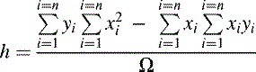
where

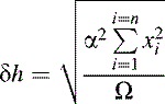
In these equations s is the scaling factor (or gradient of the response curve) and h is the transducer input required to produce an ADC reading (x) of zero. The δs and δh values are the uncertainties in s and h, respectively. It is assumed that there are n of the (xⁱ, yⁱ) calibration points.

These formulas are the basis of the PerformLinearFit() function in Listing 15.1. The various summations are performed first and the results are then used to calculate the parameters of the best-fit straight line. The Intercept variable is equivalent to the quantity h in the preceding formulas while Slope is the same as the scaling factor, s. The ErrIntercept and ErrSlope variables are equivalent to δh and δs and may be used to determine the statistical accuracy of the calibration line. The function also determines the conformance between the fitted line and the calibration points and then calculates the root-mean-square (rms) deviation (the same as α²) and worst deviation between the line and the points.

Listing 15.1. C function for performing a first-order polynomial (linear) least-squares fit to a set of calibration reference points

• #include <math.h>
• #define True 1
• #define False 0
• #define MaxNP 500 /* Maximum number of data points for fit */
• struct LinFitResults /* Results record for PerformLinearFit function */
• {
• double Slope;
• double Intercept;
• double ErrSlope;
• double ErrIntercept;
• double RMSDev;
• double WorstDev;
• double CorrCoef;
• };
• struct LinFitResults LResults;
• unsigned int NumPoints;
• double X[MaxNP];
• double Y[MaxNP];
• void PerformLinearFit()
• /* Performs a linear (first order polynomial) fit on the X[],Y[] data points and returns the results in the LResults structure.
• */
• {
• unsigned int I;
• double SumX;
• double SumY;
• double SumXY;
• double SumX2;
• double SumY2;
• double DeltaX;
• double DeltaY;
• double Deviation;
• double MeanSqDev;
• double SumDevnSq;
• SumX = 0;
• SumY = 0;
• SumXY = 0;
• SumX2 = 0;
• SumY2 = 0;
• for (I = 0; I < NumPoints; I++)
• {
• SumX = SumX + X[I];
• SumY = SumY + Y[I];
• SumXY = SumXY + X[I] * Y[I];
• SumX2 = SumX2 + X[I] * X[I];
• SumY2 = SumY2 + Y[I] * Y[I];
• }
• DeltaX = (NumPoints * SumX2) – (SumX * SumX);
• DeltaY = (NumPoints * SumY2) – (SumY * SumY);
• LResults.Intercept = ((SumY * SumX2) – (SumX * SumXY)) / DeltaX;
• LResults.Slope = ((NumPoints * SumXY) – (SumX * SumY)) / DeltaX;
• SumDevnSq = 0;
• LResults.WorstDev = 0;
• for (I = 0; I < NumPoints; I++)
• {
• Deviation = Y[I] - (LResults.Slope * X[I] + LResults.Intercept);
• if (fabs(Deviation) > fabs(LResults.WorstDev)) LResults.WorstDev = Deviation;
• SumDevnSq = SumDevnSq + (Deviation * Deviation);
• }
• MeanSqDev = SumDevnSq / (NumPoints - 2);
• LResults.ErrIntercept = sqrt(SumX2 * MeanSqDev / DeltaX);
• LResults.ErrSlope = sqrt(NumPoints * MeanSqDev / DeltaX);
• LResults.RMSDev = sqrt(MeanSqDev);
• LResults.CorrCoef = ((NumPoints * SumXY) – (SumX * SumY)) /
• sqrt(DeltaX * DeltaY);
• }

It is always advisable to check the rms and worst deviation figures when the fitting procedure has been completed, as these provide a measure of the accuracy of the fit. The rms deviation may be thought of as the average deviation of the calibration points from the straight line.

The ratio of the worst deviation to the rms deviation can indicate how well the calibration points can be modeled by a straight line. As a rule of thumb, if the worst deviation exceeds the rms deviation by more than a factor of about 3, this might indicate one of two possibilities: either the true response curve exhibits a significant nonlinearity or one (or more) of the calibration points has been measured inaccurately. Any uncertainties from either of these two sources will be reflected in the ErrorIntercept and ErrorSlope variables.

Although there is a potential for greater accuracy with multiple-point calibration, it should go without saying that the comments made in the preceding section, concerning prime-calibration accuracy, also apply to multiple-point calibration schemes.

To minimize the effect of random measurement errors, multiple-point calibration is generally to be preferred. However, it does have one considerable disadvantage: the additional time required to carry out each calibration. If a transducer is to be calibrated in situ (while attached to a machine on a production line, for example), it can sometimes require a considerable degree of effort to apply a precise reference value to the transducer's input. Some applications might employ many tens (or even hundreds) of sensors and recalibration can then take many hours to complete, resulting in project delays or lost production time. In these situations it may be beneficial to settle for the slightly less accurate two- or three-point calibration schemes. It should also be stressed that two- and three-point calibrations do often provide a sufficient degree of precision and that multiple-point calibrations are generally only needed where highly accurate measurements are the primary concern.

15.1.6. Applying Linear Scaling Parameters to Digitized Data

Once the scaling factor and offset have been determined, they must be applied to all subsequent digitized measurements. This usually has to be performed in real time and it is therefore important to minimize the time taken to perform the calculation. Obviously, high-speed computers and numeric coprocessors can help in this regard, but there are two ways in which the efficiency of the scaling algorithm can be enhanced.

First, floating-point multiplication is generally faster than division. For example, Borland Pascal's floating-point routines will multiply two real type variables in about one third to one half of the time that they would take to carry out a floating-point division. A similar difference in execution speeds occurs with the corresponding 80x87 numeric coprocessor instructions. Multiplicative scaling factors should, therefore, always be used—that is, always multiply the data by s, rather than dividing by s⁻¹— even if the software specification requires that the inverse of the scaling factor is presented on displays and printouts and the like.

Second, the scaling routines can be coded in assembly language. This is simpler if a numeric coprocessor is available, otherwise floating-point routines will have to be specially written to perform the scaling.

In very high-speed applications, the only practicable course of action might be to store the digitized ADC values directly into RAM and to apply the scaling factor(s) after the data-acquisition run has been completed, when timing constraints may be less stringent.

15.2. Linearization

Linearization is the term applied to the process of correcting the output of an ADC in order to compensate for nonlinearities present in the response curve of a measuring system. Nonlinearities can arise from a number of different components, but it is often the sensors themselves that are the primary sources.

In order to select an appropriate linearization scheme, it obviously helps to have some idea of the shape of the response curve. The response of the system might be known, as is the case with thermocouples and RTDs. It might even conform to some recognized analytical function. In some applications the deviation from linearity might be smooth and gradual, but in others the nonlinearities might consist of small-scale irregularities in the response curve. Some measuring systems may also exhibit response curves that are discontinuous or, at least, discontinuous in their first and higher-order derivatives.

There are several linearization methods to choose from and whatever method is selected, it must suit the peculiarities of the system's response curve. Polynomials can be used for linearizing smooth and slowly varying functions but are less suitable for correcting irregular deviations or sharp “corners” in the response curve. They can be adapted to closely match a known functional form or they can be used in cases where the form of the response function is indeterminate. Interpolation using lookup tables is one of the simplest and most powerful linearization techniques and is suitable for both continuous and discontinuous response curves. Each method has its own advantages and disadvantages in particular applications and these are discussed in the following sections.

The capability to linearize response curves in software can, in some cases, mean that simpler and cheaper transducers or signal-conditioning circuitry can be used. One such case is that of LVDT displacement transducers. These devices operate rather like transformers. An AC excitation voltage is applied to a primary coil and this induces a signal in a pair of secondary windings. The degree of magnetic flux linkage and, therefore, the output from each of the secondary coils is governed by the linear displacement of a ferrite core along the axis of the windings. In this way, the output from the transducer varies in relation to the displacement of the core.

Simple LVDT designs employ parallel-sided cylindrical coils. However, these exhibit severe nonlinearities (typically up to about 5 or 10%) as the ferrite core approaches the ends of the coil assembly. The nonlinearity can be corrected in a variety of ways, one of which is to layer windings in a series of steps toward the ends of the coil. This can reduce the overall nonlinearity to about 0.25%. It does, however, introduce additional small-scale nonlinearities (on the order of 0.05 to 0.10%) at points in the response curve corresponding to each of the steps.

It is a relatively simple matter to compensate for the large-scale nonlinearities inherent in parallel-coil LVDT geometries by using the polynomial linearization technique discussed in the following section. Thus, software linearization techniques allow cheaper LVDT designs to be used and this has the added advantage that no small-scale (stepped-winding) irregularities are introduced. This, in turn, makes the whole response curve much more amenable to linearization.

There are many other instances where software linearization techniques will enhance the accuracy of the measuring system and at the same time allow simpler and cheaper components to be used.

15.3. Polynomial Linearization

The most common method of linearizing the output of a measuring system is to apply a mathematical function known as a polynomial. The polynomial function is usually derived by the least-squares technique.

15.3.1. Polynomial Least-Squares Fitting

We have already seen that the technique of least-squares fitting can generate coefficients of a straight-line equation representing the response of a linear measuring system. The least-squares method can be applied to fit other equations to nonlinear response curves. The principle of the method is the same, although because we are now dealing with more complex curves and mathematical functions, the details of the implementation are slightly more involved.

A polynomial is a simple equation consisting of the sum of several separate terms. For the purposes of sensor calibration, we can define a polynomial as an equation that describes how a dynamic variable, y, such as temperature or pressure (which we intend to measure) varies in relation to the corresponding transduced signal, x (e.g., voltage output or ADC reading). Each term consists of some known function of x multiplied by an unknown coefficient.

If we can determine the coefficients of a polynomial function that closely fits a set of measured calibration reference points, it is then possible to accurately calculate a value for the physical variable, y, from any ADC reading, x.

15.3.1.1. Formulating the Best-Fit Condition

This section outlines the way in which the conditions for the best fit between the polynomial and data points can be derived. A more detailed account of this technique can be found in many texts on numerical analysis and, in particular, in the books by Miller (1993) and Press et al. (1992).

Suppose we have determined a set of calibration reference points (x¹, y¹), (x², y²), to (xⁿ, yⁿ) where the xⁱ values represent the ADC reading (or corresponding transduced voltage reading) and yⁱ are values of the equivalent “real-world” physical variable (e.g., temperature, displacement, etc.).

In certain circumstances, some of the yⁱ values will be more accurate than others and it is advantageous to pay proportionally more regard to the most accurate points. To this end, the data points can be individually weighted by a factor w^i. This is usually set equal to the inverse of the square of the known error for each point. The wⁱ terms have been included in the following account of the least-squares method, but, in most circumstances, each reference point is measured in the same way, with the same equipment, and the accuracy (and therefore weight) of each point will usually be identical. In this case all of the wⁱ values can effectively be ignored by setting them to unity.

The polynomial that we wish to fit to the (x^i,yⁱ) calibration points is (15.4)

There may be any number of terms in the polynomial. In this equation there are m + 1 terms, but it is usual for between 2 and 15 terms to be used. The number m is known as the order of the polynomial. As m increases, the polynomial is able to provide a more accurate fit to the calibration reference points. There are, however, practical limitations on m which we will consider shortly. In this equation the a^k values are a set of constant coefficients and g^k(x) represents some function of x, which will remain unspecified for the moment.

At any given order, m, the polynomial will usually not fit the data points exactly. The deviation, δⁱ, of each yⁱ reading from the fitted polynomial y′(xⁱ) value is (15.5)

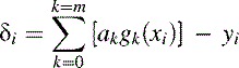
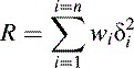
The principle of the least-squares method is to choose the a^k coefficients of the polynomial so as to minimize the sum of the squares of all δⁱ values (known as the residue). Taking into account the weights of the individual points, the residue, R, is given by (15.6)

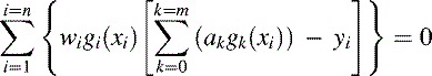
The condition under which the polynomial will most closely fit the calibration reference points is obtained when the partial derivatives of R with respect to each a^k coefficient are all zero. This statement actually represents m + 1 separate conditions which must all be satisfied simultaneously for the best fit. Space precludes a full derivation here, but with a little algebra it is a simple matter to find that each of these conditions reduces to (15.7)

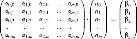
As the best-fit is described by a set of m + 1 equations of this type (for j = 0 to m), we can represent them in matrix form as follows: (15.8)

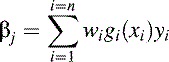
where

15.3.1.2. Solving the Best-Fit Equations

The matrix equation (15.8) represents a set of simultaneous equations that we need to solve in order to determine the coefficients, a^j, of the polynomial. The simplest method for solving the equations is to use a technique known as Gaussian elimination to manipulate the elements of the matrix and vector so that they can then be solved by simple back-substitution.

The objective of Gaussian elimination is to modify the elements of the matrix so that each position below the major diagonal is zero. This may be achieved by reference to a series of so-called pivot elements which lie at each successive position along the major diagonal. For each pivot element, we eliminate the elements below the pivot position by a systematic series of scalar-multiplication and row-subtraction operations as illustrated by the following code fragment:

• for (Row = Pivot + 1; Row <= M; Row++)
• {
• Temp = Matrix[Pivot][Row] / Matrix[Pivot][Pivot];
• for (Col = Pivot; Col <= M; Col++)
• Matrix[Col][Row] = Matrix[Col][Row] - Temp * Matrix[Col][Pivot];
• Vector[Row] = Vector[Row] - Temp * Vector[Pivot];
• }

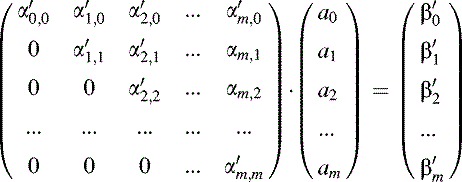
The variable M represents the order of the polynomial. Matrix is a square array with indices from 0 to M. This algorithm is used in the GaussElim() function shown in Listing 15.2 later in this chapter. Once all of the elements have been eliminated from below the major diagonal, the matrix equation will have the following form. The new matrix and vector elements are identified by primes to denote that the Gaussian elimination procedure has generated different numerical values from the original α^k;j and β^j elements. (15.9)

Listing 15.2. Fitting a power-series polynomial to a set of calibration data points

• #include <math.h>
• #define True 1
• #define False 0
• #define MaxNP 500 /* Maximum number of data points for fit */
• #define N 16 /* No. of terms. 16 accommodates 15th-order polynomial */
• struct OrderRec
• {
• long double Coef[N]; /* Polynomial coefficients */
• double RMSDev; /* RMS deviation of polynomial from Y data points */
• double WorstDev; /* Worst deviation of polynomial from Y data points */
• };
• struct PolyFitResults
• {
• unsigned char MaxOrder; /* Highest order of polynomial to fit */
• struct OrderRec ForOrder[N]; /* Polynomial parameters for each order */
• };
• struct PolyFitResults PResults;
• long double Matrix[N][N]; /* Matrix inequation 10.11*/
• long double Vector[N]; /* Vector inequation 10.11*/
• unsigned int NumPoints; /* Number of (X,Y) data points */
• double X[MaxNP]; /* X data */
• double Y[MaxNP]; /* Y data */
• long double Power(long double X, unsigned char P)
• /* Calculates X raised to the power P */
• {
• unsigned char I;
• long double R;
• R = 1;
• if (P > 0)
• for (I = 1; I <= P; I++)
• R = R * X;
• return(R);
• }
• void GaussElim(unsigned char M, long double Solution[N], unsigned char *Err)
• /* Solves the matrix equation contained in the global Matrix and Vector arrays by Gaussian Elimination and back-substitution. Returns the solution vector in the Solution array.
• */
• {
• signed char Pivot;
• signed char JForMaxPivot;
• signed char J;
• signed char K;
• signed char L;
• long double Temp;
• long double SumOfKnownTerms;
• *Err = False;
• /* Manipulate the matrix to produce zeros below the major diagonal */
• for (Pivot = 0; Pivot <= M; Pivot++)
• {
• /* Find row with the largest value in the Pivot column */
• JForMaxPivot = Pivot;
• if (Pivot < M)
• for (J = Pivot + 1; J <= M; J++)
• if (fabsl(Matrix[Pivot][J]) > fabsl(Matrix[Pivot][JForMaxPivot]))
• JForMaxPivot = J;
• /* Swap rows of matrix and vector so that the largest matrix */
• /* element is in the Pivot row (i.e. falls on the major diagonal) */
• if (JForMaxPivot != Pivot)
• {
• /* Swap matrix elements. Note that elements with K < Pivot are all */
• /* zero at this stage and may be ignored. */
• for (K = Pivot; K <= M; K++)
• {
• Temp = Matrix[K][Pivot];
• Matrix[K][Pivot] = Matrix[K][JForMaxPivot];
• Matrix[K][JForMaxPivot] = Temp;
• }
• /* Swap vector "rows" (ie. elements) */
• Temp = Vector[Pivot];
• Vector[Pivot] = Vector[JForMaxPivot];
• Vector[JForMaxPivot] = Temp;
• }
• if (Matrix[Pivot][Pivot] == 0)
• *Err = True;
• else f
• /* Eliminate variables in matrix to produce zeros in all */
• /* elements below the pivot element */
• for (J = Pivot + 1; J <= M; J++)
• {
• Temp = Matrix[Pivot][J] / Matrix[Pivot][Pivot];
• for (K = Pivot; K <= M; K++)
• Matrix[K][J] = Matrix[K][J] - Temp * Matrix[K][Pivot];
• Vector[J] = Vector[J] - Temp * Vector[Pivot];
• }
• }
• }
• /* Solve the matrix equations by back-substitution, starting with */
• /* the bottom row of the matrix */
• if (!(*Err))
• {
• if (Matrix[M][M] == 0)
• *Err = True;
• else f
• for (J = M; J >= 0; J--)
• {
• SumOfKnownTerms = 0;
• if (J < M)
• for (L = J + 1; L <= M; L++)
• SumOfKnownTerms = SumOfKnownTerms + Matrix[L][J] * Solution[L];
• Solution[J] = (Vector[J] - SumOfKnownTerms) / Matrix[J][J];
• }
• }
• }
• }
• void PolynomialLSF(unsigned char Order, unsigned char *Err)
• /* Performs a polynomial fit on the X, Y data arrays of the specified Order
• and stores the results in the global PResults structure.
• */
• {
• long double MatrixElement[2 * (N - 1) + 1]; /* Temporary storage */
• unsigned char KPlusJ; /* Index of matrix elements */
• unsigned char K; /* Index of coefficients */
• unsigned char J; /* Index of equation / vector elements */
• unsigned int I; /* Index of data points */
• /* Sum data points into Vector and MatrixElement array. MatrixElement is */
• /* used for temporary storage of elements so that it is not necessary to */
• /* duplicate the calculation of identical terms */
• for (KPlusJ = 0; KPlusJ <= (2 * Order); KPlusJ++) MatrixElement[KPlusJ] = 0;
• for (J = 0; J <= Order; J++) Vector[J] = 0;
• for (I = 0; I < NumPoints; I++)
• {
• for (KPlusJ = 0; KPlusJ <= (2 * Order); KPlusJ++)
• MatrixElement[KPlusJ] = MatrixElement[KPlusJ] + Power(X[I],KPlusJ);
• for (J = 0; J <= Order; J++)
• Vector[J] = Vector[J] + (Y[I] * Power(X[I],J));
• g
• /* Copy matrix elements to Matrix */
• for (J = 0; J <= Order; J++)
• for (K = 0; K <= Order; K++)
• Matrix[K][J] = MatrixElement[K+J];
• /* Solve matrix equation by Gaussian Elimination and back-substitution. */
• /* Store the solution vector in the Results.ForOrder[Order].Coef array. */
• GaussElim(Order,PResults.ForOrder[Order].Coef,Err);
• }
• long double PolynomialValue(unsigned char Order, double X)
• /* Evaluates the polynomial contained in the global PResults structure.
• Returns the value of the polynomial of the specified order at the
• specified value of X.
• */
• {
• signed char K;
• long double P;
• P = PResults.ForOrder[Order].Coef[Order];
• for (K = Order - 1; K >= 0; K--)
• P = P * X + PResults.ForOrder[Order].Coef[K];
• return P;
• }
• void CalculateDeviation(unsigned char Order)
• /* Calculates the root-mean-square and worst deviations of all Y values from
• the fitted polynomial.
• */
• {
• unsigned int I;
• double Deviation;
• double SumDevnSq;
• SumDevnSq = 0;
• PResults.ForOrder[Order].WorstDev = 0;
• for (I = 0; I < NumPoints; I++)
• {
• Deviation = Y[I] - PolynomialValue(Order,X[I]);
• if (fabs(Deviation) > fabs(PResults.ForOrder[Order].WorstDev))
• PResults.ForOrder[Order].WorstDev = Deviation;
• SumDevnSq = SumDevnSq + (Deviation * Deviation);
• }
• PResults.ForOrder[Order].RMSDev = sqrt(SumDevnSq / (NumPoints-2));
• }
• void PolynomialFitForAllOrders(unsigned char *Err)
• /* Performs a polynomial fit for all orders up to a maximum determined by the
• number of data points and the dimensions of the Matrix and Vector arrays.
• */
• {
• unsigned char Order;
• *Err = False;
• if (NumPoints > N)
• PResults.MaxOrder = N - 1;
• else PResults.MaxOrder = NumPoints - 2;
• for (Order = 1; Order <= PResults.MaxOrder; Order++)
• {
• if (!(*Err))
• {
• PolynomialLSF(Order,Err);
• if (!(*Err)) CalculateDeviation(Order);
• {
• {
• {

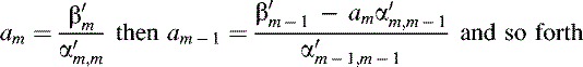
The equations represented by each row of the matrix equation can now be easily solved by repeated back-substitution. Starting with the bottom row and moving on to each higher row in sequence, we can calculate a^m then a^m – 1 then a^m – 2 and so forth as follows: (15.10)

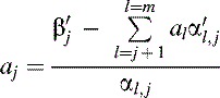
In general we have the following iterative relation which is coded as a simple algorithm at the end of the GaussElim() function in Listing 15.2: (15.11)

The curve fitting procedure would not usually need to be performed in real time and so the computation time required to determine coefficients by this method will not normally be of great importance. A 15th-order polynomial fit can be carried out in several hundred milliseconds on an average 33-MHz 80486 machine equipped with a numeric processing unit but will take considerably longer (up to a few seconds, depending upon the machine) if a coprocessor is not used. The total calculation time increases roughly in proportion to cube of the matrix size.

A number of other methods can be used to solve the matrix equation. These may be preferable if Gaussian elimination fails to provide a solution because the coefficient matrix is singular or if rounding errors become problematic. A discussion of these techniques is beyond the scope of this book. Press et al. (1992) provide a detailed description of curve fitting methods together with a comprehensive discussion of their relative advantages and drawbacks.

15.3.1.3. Numerical Accuracy and Ill-Conditioned Matrices

All computer-based numerical calculations are limited by the finite accuracy of the coprocessor or floating-point library used. Gaussian elimination involves many repeated multiplications, divisions, and subtractions. Consequently rounding errors can begin to accumulate, particularly with higher-order polynomials. While single-precision arithmetic is suitable for many of the calculations that we have to deal with in data-acquisition applications, it does not usually provide sufficient accuracy for polynomial linearization. When undertaking this type of calculation, it is generally beneficial to use floating-point data types with the greatest possible degree of precision. The examples presented in this chapter use C's long double data type, which is the largest type supported by the 80x87 family of numeric coprocessors.

Even when using the long double data type, rounding errors can become significant when undertaking Gaussian elimination. For this reason it is generally inadvisable to attempt this for polynomials of greater than about 15th order. In some cases, rounding errors may also be important with lower-order polynomials. If the magnitudes of the pivot elements vary greatly along the major diagonal, the process of Gaussian elimination may cause rounding errors to build up to a significant level and it will then be impossible to calculate accurate values for the polynomial coefficients. The accuracy of the Gaussian elimination method can be improved by first swapping the rows of the matrix equation so that the element in the pivot row with the largest absolute magnitude is placed in the pivot position on the major diagonal. This minimizes the difference between the various pivot elements and helps to reduce the effect of rounding errors on the calculations.

If one of the pivot elements is zero, the matrix equation cannot be solved by Gaussian elimination. If one or more of the pivot elements are very close to zero, the solution of the matrix equation may generate very large polynomial coefficients. Then when we subsequently evaluate the polynomial, the greatest part of these coefficients tend to cancel each other out, leaving only a small remainder that contributes to the actual evaluation. This is obviously quite susceptible to numerical rounding errors.

The combination of elements in the matrix might be such that rounding errors in some of the operations performed during the elimination procedure become comparable with the true result of the operation. In this case the matrix is said to be ill-conditioned and the solution process may yield inaccurate coefficients.

It is usually advisable to check for ill-conditioned matrices by examining the pivot elements along the major diagonal to ensure that they do not differ by very many orders of magnitude. Obviously, if higher-precision data types are used for calculation and storage of results (e.g., extended or double precision rather than single precision), it is possible to accommodate a greater range of values along the major diagonal.

It is also possible to detect the effect of ill-conditioned matrices and rounding errors after the fit has been performed. This can be achieved by carrying out conformance checks, as des335bed in the next subsection, for a range of polynomial orders. This is not a foolproof technique, but in general, the root-mean-square deviation between the calibration reference points and the fitted polynomial will tend to increase with increasing order once rounding errors become significant.

15.3.1.4. Accuracy of the Fitted Curve

In the absence of any appreciable rounding errors, the accuracy with which the polynomial will model the measuring system's response curve will be determined by two factors: the magnitude of any random or systematic measurement errors in the calibration reference points and the “flexibility” of the polynomial.

Although the effect of random errors can be offset to some extent by taking a larger number of calibration measurements, any systematic errors cannot generally be determined or corrected during linearization and so must be eliminated at source. There are many possible sources of random error. Electrical noise can be a problem with low-voltage signals such as those generated by thermocouples. There are also often difficulties in setting the measurand to a precise enough value, especially where the sensor is an integral part of a larger system and has to be calibrated in situ. Whatever the source of a random error, it generally introduces some discrepancy between the true response curve and the measured calibration reference points.

A second source of inaccuracy might arise where the polynomial is not flexible enough to fit response curves with rapidly changing gradients or higher derivatives. Better fits can usually be achieved by using high-order polynomials, but as mentioned previously, rounding errors can become problematic if very high orders are used.

Whenever a polynomial is fitted to a set of calibration reference points it is essential to obtain some measure of the accuracy of the fit. We can determine the uncertainties in the coefficients if we solve the best-fit equation (15.8) by the technique of Gauss-Jordan elimination. As part of the Gauss-Jordan elimination procedure, we determine the inverse of the coefficient matrix and this can be used to calculate the uncertainties in the coefficients. The Gauss-Jordan method is somewhat more involved than Gaussian elimination and, apart from providing an easy means of calculating the coefficient errors, has no other advantage. This method is discussed by Press et al. (1992) and will not be described here.

A simpler way of estimating the accuracy of the fit is to calculate the conformance between the fitted curve and each calibration reference point. We simply evaluate the polynomial y′(xⁱ) for each xⁱ value in turn and then determine the deviation of the corresponding measured yⁱ value from the polynomial (see Equation [15.5]). This is illustrated by the following code fragment:

• SumDevnSq = 0;
• WorstDev = 0;
• for (I = 0; I < NumPoints; I++)
• {
• Deviation = Y[I] - PolynomialValue(Order,X[I]);
• if (fabs(Deviation) > fabs(WorstDev)) WorstDev = Deviation;
• SumDevnSq = SumDevnSq + (Deviation * Deviation);
• }
• RMSDev = sqrt(SumDevnSq / (NumPoints-2));

In this example, the polynomial is evaluated for the Ith data point by calling the PolynomialValue() function (which will, of course, vary depending upon the functional form of the polynomial). A function of this type for evaluating a power-series polynomial is included in Listing 15.2 later in this chapter.

It is important not to rely too heavily on the conformance values calculated in this way. They show only how closely the polynomial fits the calibration reference points and do not indicate how the polynomial might vary from the true response curve between the points. It is advisable to check the accuracy of the polynomial at a number of points in between the original calibration reference points.

15.3.1.5. Choosing the Optimum Order

In general the higher the order of the polynomial, the more closely it will fit the calibration reference points. One might be tempted always to fit a very high-order polynomial, but this has several disadvantages. First, high-order polynomials take longer to evaluate, and as the evaluation process is likely to be carried out in real time, this can severely limit throughput. Second, rounding errors tend to be more problematic with higher-order polynomials as already discussed. Finally, more calibration reference points are required in order to obtain a realistic approximation to the response curve.

For any polynomial fit, the number of calibration reference points used must be greater than m + 1, where m is the order of the polynomial. If this rule is broken, by choosing an order that is too high, the fitting procedure will not provide accurate coefficients and the polynomial will tend to deviate from a reasonably smooth curve between adjacent data points. In order to obtain a smooth fit to the response curve it is always advisable to use as many calibration reference points as possible and the lowest order of polynomial consistent with achieving the required accuracy. As the order of the fit is increased, the rms deviation between the fitted polynomial and the reference points will normally tend to decrease and then level out as shown in Figure 15.2.

Figure 15.2. Typical rms deviation vs. order for a power-series polynomial fit.

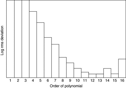
The shape of the graph will, of course, vary for different data sets, but the same general trends will usually be obtained. In this example, there is little to be gained by using an order greater than about 11 or 12. At higher orders rounding errors may begin to come into play causing the rms deviation to rise irregularly. If the requirements of an application are such that a lower degree of accuracy would be acceptable, it is generally preferable to employ a lower-order polynomial, for the reasons mentioned already.

15.3.2. Linearization with Power-Series Polynomials

So far, in the discussion of the least-squares technique, the form of the g^k(x) function has not been specified. In fact, it may be almost any continuous function of x such as sin(x), ln(x), and so on. For correcting the response of a nonlinear sensor, it is usual to use a power-series polynomial where each successive term is proportional to an increasing power of x. For a power-series polynomial, the elements of the matrix and vector in Equation (15.11) become (15.12)

By setting all weights to unity, substituting these elements into the matrix equation for a first-order polynomial, and then solving for a⁰ and a¹, we can arrive at Equations (15.3) for the parameters of a straight line which were presented in Section 15.1.5, Multiple-Point Prime Calibration. (Note that the following substitutions must be made: a¹ = s; a⁰ = h.)

Power-series polynomials are a special case of the generalized polynomial function fit and are useful for correcting a variety of nonlinear response curves. They are, perhaps, most often employed for linearizing thermocouple signals but they can also be used with a number of other types of nonlinear sensor. The resistance vs. temperature characteristic of a platinum RTD, for example, can be linearized with a second-order power-series polynomial (Johnson, 1988), but for higher accuracy or wider temperature ranges, a third- or fourth-order polynomial should be used. Higher- (typically 8th- to 14th-) order polynomials are required to linearize thermocouple signals, as the response curves of these devices tend to be quite nonlinear. Power-series polynomials are most effective where the response curve deviates smoothly and gradually from linearity (as is usually the case with thermocouple signals), but they normally provide a poorer fit to curves that contain sudden steps, bumps, or discontinuities.

Nonlinearities often stem from the design of the transducer and its associated signal conditioning circuits. However, power-series polynomials can also be used in cases where other sources of nonlinearity are present. For example, the mechanical design of a measuring system might require a displacement transducer such as an LVDT to be operated via a series of levers in order to indirectly measure the rotational angle of some component. In this case, although the response of the LVDT and signal conditioning circuits are essentially linear, the transducer's output will have a nonlinear relation to the quantity of interest. Systems such as this often exhibit smooth deviations from linearity and can usually be linearized with a power-series polynomial.

15.3.2.1. Fitting a Power-Series Polynomial

To fit a polynomial of any chosen order to a set of calibration reference points, it is first necessary to construct a matrix equation with the appropriate terms (as defined by Equation (15.1)). The matrix should be simplified using the Gaussian elimination technique described in the previous section and the coefficients may then be calculated by back-substitution.

Listing 15.2 shows how a power-series polynomial can be fitted to an unweighted set of calibration reference points. As each point is assumed to have been determined to the same degree of precision, all weights in Equations (15.12) can be set to unity. If required, weights could easily be incorporated into the code by modifying the first block of lines in the PolynomialLSF() function.

The code in this listing will automatically attempt to fit polynomials of all orders up to a maximum order which is limited by either the matrix size or the number of available calibration points. The present example accommodates a 16 × 16 matrix which is sufficient for a 15th-order polynomial. If necessary, the size of the matrix can be increased by modifying the #define N line. Bear in mind, however, that if larger matrices and polynomials are used, rounding errors may become problematic. As mentioned in the previous section, polynomial fits should not be attempted for orders greater than n – 2, where n represents the number of calibration reference points. The code will, therefore, not attempt to fit a polynomial if there are insufficient points available.

The (xⁱ, yⁱ) data for the fit are made available to the fitting functions in the global X and Y arrays. The results of the fitting are stored in the global PResults structure (of type PolyFitResults). The PolynomialFitForAllOrders() function performs a polynomial fit to the same data over a range of orders by calling the PolynomialLSF() function once for each order. This constructs the matrix and vector defined in Equation (15.11) using the appropriate power-series polynomial terms and then calls the GaussElim() function to solve the matrix equation. After each fit has been performed, the CalculateDeviation() function determines the rms and worst deviation of the (xⁱ, yⁱ) points from the fitted curve.

All of the fitting calculations employ C's 80-bit long double floating-point data type. This is the same as Pascal's extended type and corresponds to the Intel 80x87 coprocessor's Temporary Real data type. These provide 19 to 20 significant digits over a range of about 3.4 × 10⁻⁴⁹³² to 1.1 × 10⁺⁴⁹³².

The listing incorporates two functions that are actually included in some standard C libraries. Calls to the Power() function can be replaced by calls to the C powl() function if it is supported in your library. The function has been included here for the benefit of readers who wish to translate the code into languages, such as Pascal, that might not have a comparable procedure.

Users of Borland C++ or Turbo C/C++ may wish to replace the PolynomialValue() function with the poly() or polyl() library functions. However, these are not defined in ANSI C and are not supported in all implementations of the language.

15.3.2.2. Evaluating a Power-Series Polynomial

In order to calculate the rms and worst deviation, it is necessary for the code to evaluate the fitted polynomial for each of the xⁱ values. The most obvious way to do this would have been to calculate each term individually and to sum them as follows:

• PolyValue = 0;
• for (K = 0; K <= Order; K++)
• PolyValue = PolyValue + Coef[K]*Power(X[I],K);

However, this requires x^ik to be evaluated for each term, which results in many multiplication operations being performed unnecessarily by the Power() function. The following algorithm is much more efficient and requires only Order + 1 multiplications to be performed. Note that the index K is, in this case, a signed char.

• PolyValue = Coef[Order];
• for (K = Order-1; K >= 0; K--)
• PolyValue = PolyValue * X[I] + Coef[K];

For a 15th-order polynomial the first method requires 121 separate multiply operations while only 16 are needed in the more efficient second method. The second method minimizes the effect of rounding errors and will often make a significant improvement to throughput.

15.3.3. Polynomials in Other Functions

A power-series polynomial can be useful where the functional form of a response curve is unknown or difficult to determine. However, the response of some measuring systems might clearly follow a combination of simple mathematical functions (sin, cos, log, etc.) and in such cases it is likely that a low-order polynomial in the appropriate function will provide a more accurate fit than a high-order power-series polynomial.

Thermistors, for example, exhibit a resistance (R) vs. temperature (T) characteristic in which the inverse of the temperature is proportional to a polynomial in ln R (see Tompkins and Webster, 1988): (15.13)

A response curve based on a simple mathematical function might also arise where the nonlinearity is introduced by the geometry of the measuring system. One example is that of level measurement using a float and linkage as shown in Figure 15.3.

Figure 15.3. Measurement of fluid level using a float linked to a rotary potentiometer.

The float moves up and down as the level of liquid in the tank changes and the resulting motion (i.e., angle a) of the mechanical link is sensed by a rotary potentiometric transducer. The output of the potentiometer is assumed to be proportional to a, and the level, h, of liquid in the tank will be approximately proportional to cos(a).

The best approach might initially seem to be to scale the output of the potentiometer to obtain the value of a and then apply the simple cos(a) relationship in order to calculate h. This might indeed be accurate enough, but we should remember that there may be other factors that affect the actual relationship between h and the potentiometer's output. For example, the float might sit at a slightly different level in the liquid depending upon the angle a and this will introduce a small deviation from the ideal cosinusoidal response curve. Deviations such as this are usually best accounted for by performing a prime calibration and then linearizing the resulting calibration points with the appropriate form of polynomial.

The polynomial fitting routine in Listing 15.2 can easily be modified to accommodate functions other than powers of x. There are only two changes which usually need to be made. The first is that the PolynomialLSF() function should be adapted to calculate the matrix elements from the appropriate g^k(x) functions. The other modification required is in the three lines of code in the PolynomialValue() function which evaluates the polynomial at specific points on the response curve.

15.4. Interpolation between Points in a Lookup Table

Suppose that a number of calibration points, (x¹, y¹), (x², y²), to (xⁿ, yⁿ), have been calculated or measured using the prime calibration techniques discussed previously. If there are sufficient points available, it is possible to store them in a lookup table and to use this table to directly convert the ADC reading into the corresponding “real-world” value. In cases where a low-resolution ADC is in use, it might be feasible to construct a table containing one entry for each possible ADC reading. This, however, requires a large amount of system memory, particularly if there are several ADC channels, and it is normally only practicable to store more widely separated reference points. In order to avoid having to round down (or up) to the nearest tabulated point, it is usual to adopt some method of interpolating between two or more neighboring points.

15.4.1. Sorting the Table of Calibration Points

The first step in finding the required interpolate is to determine which of the calibration points the interpolation should be based on. Two (or more) points with x values spanning the interpolation point are required, and the software must undertake a search for these points. In order to maximize the efficiency of the search routine (which often has to be executed in real time), the data should previously have been ordered such that the x values of each point increase (or decrease) monotonically through the table.

The points may already be correctly ordered if they have been entered from a published table or read in accordance with a strict calibration algorithm. However, this may not always be the case. It is prudent to provide the operator with as much flexibility as possible in performing a prime calibration and this may mean relaxing any constraints on the order in which the calibration points are entered or measured. In this case it is likely that the lookup table will initially contain a randomly ordered set of measurements that will have to be rearranged into a monotonically increasing or decreasing sequence.

One of the most efficient ways of sorting a large number (up to about 1000) of disordered data points is shown in Listing 15.3. This is based on the Shell-Metzner sorting algorithm (Knuth, 1973; Press et al., 1992) and arranges any randomly ordered table of (x, y) points into ascending x order.

Listing 15.3. Sorting routine based on the Shell-Metzner (shell sort) algorithm for use with up to approximately 1000 data points

• #define True 1
• #define False 0
• #define MaxNP 500 /* Maximum number of data points in lookup table */
• void ShellSort(unsigned int NumPoints, double X[MaxNP], double Y[MaxNP])
• /* Sorts the X and Y arrays according to the Shell-Metzner algorithm so that
• the contents of the X array are placed in ascending numeric order. The
• corresponding elements of the Y array are also interchanged to preserve the
• relationship between the two arrays.
• */
• {
• unsigned int DeltaI; /* Separation between compared elements */
• unsigned char PointsOrdered; /* True indicates points ordered on each pass */
• unsigned int NumPairsToCheck; /* No. of point pairs to compare on each pass */
• unsigned int I0,I; /* Indices for search through arrays */
• double Temp; /* Temporary storage for swapping points */
• if (NumPoints > 1)
• {
• DeltaI = NumPoints;
• do
• {
• DeltaI = DeltaI / 2;
• /* Compare pairs of points separated by DeltaI */
• do
• {
• PointsOrdered = True;
• NumPairsToCheck = NumPoints - DeltaI;
• for (I0 = 0; I0 < NumPairsToCheck; I0++);
• {
• I = I0 + DeltaI;
• if (X[I0] > X[I])
• {
• /* Swap elements of X array */
• Temp = X[I];
• X[I] = X[I0];
• X[I0] = Temp;
• /* Swap elements of Y array */
• Temp = Y[I];
• Y[I] = Y[I0];
• Y[I0] = Temp;
• PointsOrdered = False; /* Not yet ordered so do same pass again */
• }
• }
• }
• while (!PointsOrdered);
• }
• while (DeltaI != 1);
• }
• }

The ShellSort() function works by comparing pairs of x values during a number of passes through the data. In each pass the compared values are separated by DeltaI array locations and DeltaI is halved on each successive pass. The first few passes through the data introduce a degree of order over a large scale and subsequent passes reorder the data on continually smaller and smaller scales.

This might seem to be an unnecessarily complicated method of sorting, but it is considerably more efficient than some of the simpler algorithms (such as the well-known search-and-insert or bubble sort routines), particularly if the data set contains more than about 30 to 40 points. The time required to execute the ShellSort() algorithm increases in proportion to NumPoints to the power of 1.5 or less, while the execution time for a bubble sort increases with NumPoints squared. However, if there are only a small number of calibration points (less than about 20 to 30) to be sorted, the simpler BubbleSort() routine shown in Listing 15.4 will generally execute faster than ShellSort().

Listing 15.4. Bubble Sort routine for use with fewer than approximately 20 to 30 data points

• #define MaxNP 500 /* Maximum number of data points in lookup table */
• void BubbleSort(unsigned int NumPoints, double X[MaxNP], double Y[MaxNP])
• /* Sorts the X and Y arrays according to the Bubble Sort algorithm so that the contents of the X array are placed in ascending numeric order. The corresponding elements of the Y array are also interchanged to preserve the relationship between the two arrays.
• */
• {
• unsigned int I;
• unsigned int I0;
• double Temp;
• for (I0 = 0; I0 < NumPoints - 1; I0++)
• {
• for (I = I0 + 1; I < NumPoints; I++)
• {
• if (X[I0] > X[I])
• {
• /* Swap elements of X array */
• Temp = X[I];
• X[I] = X[I0];
• X[I0] = Temp;
• /* Swap elements of Y array */
• Temp = Y[I];
• Y[I] = Y[I0];
• Y[I0] = Temp;
• }
• }
• }
• }

The C language includes a qsort() function which can be used to sort an array of data according to the well-known Quick Sort algorithm. This algorithm is ideal when dealing with large quantities of data (typically >1000 items), but for smaller arrays of calibration points, a well-coded implementation of the Shell-Metzner technique tends to be more efficient.

The bubble sort algorithm is notoriously inefficient and should be used only if the number of data points is small. Do not be tempted to use a routine based on the bubble sort method with more than about 20 to 30 points. It becomes very slow if large tables of data have to be sorted, and in these cases, it is worth the slight extra coding effort to replace it with the Shell Sort routine.

There are many other types of sorting algorithm. Most of these are, however, designed specially for sorting very large quantities of data and there is usually no significant advantage to be gained by using them in preference to the ShellSort() function. See Press et al. (1992) and Knuth (1973) for more detailed discussions of this topic.

The sorting process should, of course, be performed immediately after the calibration reference points have been entered or measured. It should not be deferred until run time as this is likely to place an unacceptable burden on the real-time operation of the software.

15.4.2. Searching the Lookup Table

In order to determine which calibration points will be used for the interpolation, the software must search the previously ordered table. The most efficient searching routines tend to be based on bisection algorithms such as that identified by the Bisection Search comment in Listing 15.5. This routine searches through a portion of the table (defined by the indices Upper and Lower) by repeatedly halving it. It decides which portion of the table is to be bisected next by comparing the bisection point (Bisect) with the required interpolation point (TargetX). The bisection algorithm rapidly converges on the pair of data points with x values spanning TargetX and returns the lower of the indices of these two points. This is similar, in principle, to the successive-approximation technique employed in some analog-to-digital converters.

Listing 15.5. Delimit-and-bisect function for searching an ordered table

• #define True 1
• #define False 0
• #define MaxNP 500 /* Maximum number of data points in lookup table */
• void Search(unsigned int NumEntries, double X[MaxNP], double TargetX,
• signed int *Index, unsigned char *Err)
• /* Searches the ascending table of X values by bracketing and then bisection. This procedure will not accommodate descending tables. NumEntries specifies the number of entries in the X array and should always be less than 32768. Bracketing starts at the entry specified by Index. The bisection search then returns the index of the entry such that X[Index] <= TargetX < X[Index+1]. If Index is out the range 1 to NumEntries, the bisection search is performed over the whole table. If TargetX < X[1] or TargetX >= X[NumEntries], Err is set true.
• */
• {
• signed int Span;
• signed int Upper;
• signed int Lower;
• unsigned int Bisect;
• if (X[0] > X[NumEntries-1])
• *Err = True; /*Descending*/
• else *Err = ((TargetX < X[0]) ∣∣ (TargetX >= X[NumEntries-1])); /*Ascending*/
• if (!*Err)
• {
• /* Define search limits */
• if ((*Index >= 0) && (*Index < NumEntries))
• {
• /* Adjust bracket interval to encompass TargetX */
• Span = 1;
• if (TargetX >= X[*Index])
• {
• /* Adjust upward */
• Lower = *Index;
• Upper = Lower + 1;
• while (TargetX >= X[Upper])
• {
• Span = 2 * Span;
• Lower = Upper;
• Upper = Upper + Span;
• if (Upper > NumEntries - 1) Upper = NumEntries - 1;
• }
• }
• else f
• /* Adjust downward */
• Upper = *Index;
• Lower = Upper - 1;
• while (TargetX < X[Lower])
• {
• Span = 2 * Span;
• Upper = Lower;
• Lower = Lower - Span;
• if (Lower < 0) Lower = 0;
• }
• }
• }
• else {
• /* *Index is out of range so search the whole table */
• Lower = 0;
• Upper = NumEntries;
• }
• /* Bisection search */
• while ((Upper - Lower) > 1)
• {
• Bisect = (Upper + Lower) / 2;
• if (TargetX > X[Bisect])
• Lower = Bisect;
• else Upper = Bisect;
• }
• *Index = Lower;
• }
• }

The total execution time of the bisection search algorithm increases roughly in proportion to log²(n), where n is the number of points in the range of the table to be searched.

The bisection routine would work reasonably well if the Upper and Lower search limits were to be set to encompass the whole table, but this can often be improved by including code to define narrower search limits. The reason is that, in many data-acquisition applications, there is a degree of correlation between successive readings. If the signal changes slowly compared to the sampling rate, each consecutive reading will be only slightly different from the previous one. The Search() function takes advantage of any such correlation by starting the search from the last interpolation point. It initially sets the search range so that it includes only the last interpolation point (x value) used and then continuously extends the range in the direction of the new interpolation point until the new point falls within the limits of the search range. The final range is then used to define the boundaries of the subsequent bisection search.

The Search() function uses the initial value of the Index parameter to fix the starting point of the range-adjustment process. The calling program should usually initialize Index before invoking Search() for the first time and it should subsequently ensure that Index retains its value between successive calls to Search(). It is, of course, possible to cause the searching process to begin at any other point in the table just by setting Index to the required value before calling the Search() function.

If successive readings are very close, the delimit-and-bisect strategy can be considerably more efficient than always performing the bisection search across the whole table. The improvement in efficiency is most noticeable in applications that use extensive calibration tables. However, if successive readings are totally unrelated, this method will take approximately twice as long (on average) to find the required interpolation point.

The Search() function will work only on tables in which the x values are arranged in ascending numerical order, but it can easily be adapted to accommodate descending tables.

15.4.3. Interpolation

There are many types of interpolating function—the nature of each application will dictate which function is most appropriate. The important point to bear in mind when selecting an interpolating function is that it must be representative of the true form of the response curve over the range of interpolation. The present discussion will be confined to simple polynomial interpolation which (provided that the tabulated points are close enough) is a suitable model for many different shapes of response curve.

Any n adjacent calibration points describe a unique polynomial of order n – 1 that can be used to interpolate to any other point within the range encompassed by the calibration points. Lagrange's equation describes the interpolating polynomial of order n – 1 passing through any n points, (x¹, y¹), (x², y²), …, (xⁿ, yⁿ): (15.14)

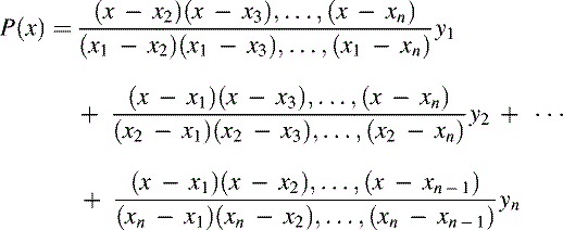
The Lagrange polynomial can be evaluated at any point, xⁱ, where 1 ≤ i ≤ n, in order to provide an estimate of the true response function y (xⁱ).

The interpolating polynomial should not be confused with the best-fit polynomial determined by the least-squares technique. The (n – 1)th order interpolating polynomial passes precisely through the n reference points; the best-fit polynomial represents the closest approximation that can be made to the reference points using a polynomial of a specified order. In general the order of the best-fit polynomial is considerable smaller than the number of data points.

It is usually not advisable to use a high- (i.e., greater than about fourth- or fifth-) order interpolating polynomial either, unless there is a good reason to believe that it would accurately model the real response curve. High-order polynomials can introduce an excessive degree of curvature. They also rely on reference points that are more distant from the required interpolation point and these are, of course, less representative of the required interpolate.

The other important drawback with high-order polynomial interpolation is that it involves quite complex and time-consuming calculations. As the interpolation usually has to be performed in real time, we are generally restricted to using low-order (i.e., linear or quadratic) polynomials. The total execution time can be reduced if the calibration reference points are equally spaced along the x axis. We can see from Lagrange's equation that, in this case, it would be possible to simplify the denominators of each term and thus to reduce the number of arithmetic operations involved in performing the interpolation.

In order to avoid compromising the accuracy of the calibration, it is necessary to ensure that sufficient calibration reference points are contained within the lookup table. The points should be more closely packed in regions of the response curve that have rapidly changing first derivatives.

If the points are close enough, we can use the following simple linear interpolation formula: (15.15)

A number of other interpolation techniques exist and these may occasionally be useful under special circumstances. For a thorough discussion of this topic, the reader is referred to the texts by Fröberg (1966) and Press et al. (1992).

15.5. Interpolation vs. Power-Series Polynomials

Interpolation can in some circumstances provide a greater degree of accuracy than linearization schemes that are based on the best-fit polynomial. A 50-point lookup table will approximate the response of a type-T thermocouple to roughly the same degree of accuracy as a 12th-order polynomial. It is relatively easy to increase the precision of a lookup table by including more points, but increasing the order of a linearizing polynomial can be less straightforward because of the effect of rounding errors.

Interpolation using a lookup table can also be somewhat faster than evaluating the best-fit polynomial, particularly if the PC is not equipped with a numeric coprocessor. The speed advantage obtained with lookup tables will, of course, depend upon the number of points in the table and the order of the polynomial. The time required to evaluate a power-series polynomial increases in proportion to its order. Using the Search() function in Listing 15.5, the total search time required prior to performing an interpolation increases approximately in proportion to log2(η) where η represents the average number of elements to be searched. As mentioned previously, if successive readings are correlated, η can be quite small. As a rough rule of thumb, if a numeric coprocessor is used, it takes about the same length of time to evaluate a 12th-order polynomial as to search a 25-point table and then perform a linear interpolation. If a coprocessor is not available, the balance will tend to shift in favor of the search-and-interpolate technique.

15.6. Interactive Calibration Programs

The users of a data-acquisition program will probably be familiar with the measurements that it will be required to make. Indeed, it is quite possible that the software will have been commissioned in order to computerize some process that the operator has already been carrying out for a number of years. The calibration procedure is not generally related to the logic of the data-acquisition process, and consequently, the end user is probably less likely to understand the steps involved in calibration than any other part of the measuring system. Calibration often requires quite a high degree of operator involvement. Any mistakes will have the potential to introduce serious errors into the measuring system and may disrupt the system's control functions.

For these reasons, calibration can be one of the most problematic aspects of a data-acquisition system and it is worthwhile making the calibration software as efficient, informative, and easy to use as possible. This benefits not only the end user but also the supplier in fewer maintenance call-outs and telephone queries.

From the programmer's point of view, the simplest calibration routines are those that require the user to calculate scaling factors, offsets, or polynomial coefficients and to type in these values for subsequent storage in a data file. Clearly, this procedure can be quite error prone. A more satisfactory alternative it to produce an interactive calibration program that continuously displays the output from the sensor and, when commanded to do so, samples the ADC output and automatically calculates scaling factors or linearization parameters. This reduces the operator's job to simply adjusting the sensor input and/or the signal-conditioning (e.g., amplifier gain) and then selecting the appropriate menu options on the PC. Whatever method is chosen, it cannot be overemphasized that the calibration program should be as simple to use as possible and should minimize the potential for operator errors.

15.6.1. The User Interface

The computer should, as far as possible, oversee the sequence of events that occur during the calibration process. The software might, for example, require the transducer's zero offset to be measured first and a second calibration reference point to be obtained at the transducer's full-scale setting. It is, however, advisable to provide the operator with the option to abandon the calibration procedure and to either restart the whole process or to restore the scaling factor and other calibration parameters to their original values.

The calibration program's display screen should be as clear and informative as possible. Large digital displays might be used to indicate the current scaled and unscaled sensor readings, while analog bar charts can provide a more graphic representation. Different colors can be used for the scaled and unscaled displays in order to enhance clarity. It is sometimes useful to change the colors of the displays whenever the input is scaled or linearized, thereby shifting the visual emphasis from one set of indicators to the other. Other useful facilities might include a noise-monitoring facility to ensure that the level of noise present will not compromise calibration accuracy.

The calibration software should be designed to trap operator errors wherever possible. It should, for example, detect when obviously incorrect inputs are applied to the transducer. Clear on-screen instructions, information panels, and help screens are of considerable value. Diagrams or other pictorial representations of the positions or status of the various sensors can also be a useful aid to understanding the calibration process.

15.7. Practical Issues

Calibration is usually a straightforward matter if easy access is available to the sensor and if it is possible to use the appropriate type of measuring jig or calibration reference device. In many situations, however, the transducer forms part of a larger system—perhaps part of a machine working on a production line—and in these cases the transducer may have to be calibrated in situ. This often introduces a number of practical difficulties into the calibration process. By designing the software to take account of these difficulties it is possible to greatly simplify the procedures involved in calibration. A few of the relevant considerations are described next.

15.7.1. Flexible Calibration Sequence

At its simplest, prime calibration involves the following steps:

1. Sample the output of the measuring system with zero input
2. Sample the output of the measuring system at (or near to) full scale
3. Calculate the offset and scaling factor from the two previous calibration points

Each of these steps may be performed in response to specific inputs from the user (e.g., a key press, menu selection, or mouse click). Obviously, three-point and multiple-point calibration schemes would require more than two reference points to be obtained, but the basic principle still applies.

It should be borne in mind that, in multichannel systems, there may be a correlation between the readings obtained with two or more of the sensors—that is, the various sensors might actually measure different aspects of the same physical process or object. For example, consider a system that uses 100 LVDTs in a gauging jig to measure the displacement at different locations on the surface of some manufactured component. It might be difficult to individually set each transducer to its zero position and then to its full-scale position using a set of gauge blocks. A more practical method would be to place two dummy components, or spacers, inside the jig: one to define each of the two calibration reference points. In this case, the zero-level spacer would be inserted, to set all transducers to their respective zero levels, and step 1 would be carried out for each transducer in turn. A similar sequence would then be performed with a different spacer for step 2 and so on.

The calibration program should not, in this case, assume that the whole calibration procedure will be completed for each transducer in turn. The user should be allowed to change sensor channels at any stage between the various calibration steps, in order to begin calibrating another channel. At some later time the user should then be able to resume calibration of the original channel.

15.7.2. Offset Correction

As mentioned previously, there are many possible sources of offset, some of which might change over time or with successive repetitions of a measuring process. Offsets can be introduced by factors such as tare weights of containers or other variables that affect the baseline of the measured quantity.

Most measuring systems should be recalibrated periodically. Fortunately, the sensitivity and linearity of many systems remains fairly constant, and in these cases, it may be sufficient to check only for variations in the offset in each channel. This facility is essential in dimensional gauging systems such as that described in the previous section. In these systems a master or reference component is periodically placed in the gauging jig so that the software can measure and subtract out any offsets that might be caused by thermal expansion or sensor movement and the like.

If possible, the data-acquisition program should repeatedly check for any drifts that might have occurred in the zero offset of each sensor. This is most easily accomplished in systems that perform repetitive tasks (e.g., component assembly machines on a production line) where the measurand returns to some known starting value after each measuring cycle is completed. This value can be compared on successive cycles in order to detect and correct for any changes in offset.

15.7.3. Generating a Precise Measurand

Prime calibration requires that the output of the measuring system is determined for a number of precisely known values of the measurand. However, it is sometimes impracticable for the sensor's input to be set precisely to any fixed value (e.g., the full-scale limit of the measuring system). In such cases it is clearly undesirable for the calibration software to require any specific value of the measurand to be applied, and the operator should be allowed some leeway in selecting or adjusting the calibration reference levels.

The following example may illustrate this point. Suppose that an LVDT displacement transducer is attached to a hydraulic arm. While the operator can accurately measure the displacement of the transducer's armature, it might be difficult to adjust the position of the hydraulic arm with the degree of precision needed to bring about any specific displacement. If, during a calibration sequence, a reference point must be obtained near to the end of the transducer's range, it would be preferable for the software to allow the operator to set the calibration point anywhere within, perhaps, 90–100% of full scale, rather than demanding that the transducer is set precisely to full scale. Provided that the operator enters the value of the calibration point actually used, the software should be able to account for the difference between the ideal and actual values of the measurand when calculating the scaling factor.

15.7.4. Remote Indication and Control

Interactive calibration is normally straightforward provided that the PC is located close to the measuring system, but if the sensors happen to be positioned in a separate room or high up on the support pillars of a bridge, for example, this procedure can be highly impracticable. The operator may be unable to see any visual display of the sensor's output on the computer's screen. It may also be difficult to continually move between the sensor and PC during the calibration process. However, with a little foresight, the programmer or system designer can circumvent such difficulties with features such as extra large displays, audible indicators, remote keypads, or remote numeric indicators or simply by using a portable PC.

15.7.5. Security

It is often important to restrict access to the measuring system's calibration facilities. This can be achieved by means of password protection schemes and file encryption techniques. In some applications security can be enhanced by appropriate choice of operating system. A discussion of these topics is unfortunately beyond the scope of this book, but Grover (1989) provides a useful overview of cryptography and software security issues in general.

15.7.6. Traceability

It is quite often necessary, for quality assurance purposes, to record precise details of every calibration performed. The identity of the operator who performed the calibration procedure might have to be recorded along with the calibration data itself. It is also usually essential to record which instrument or gauge has been used as the prime calibration reference so that the whole calibration is traceable to a higher-level standard. Collet and Hope (1983) discuss the subject of traceability in greater detail.