Chapter 23. Test Methods

The major part of all the basic standards consists of recipes for carrying out the tests. Because the values obtained from measurements at radio frequency (RF) are so dependent on layout and method, these have to be specified in some detail to generate a standard result. This chapter summarizes the issues involved in full compliance testing, but to actually perform the tests you are recommended to consult the relevant standard carefully.

23.1. Test Setup

23.1.1. Layout

23.1.1.1. Conducted Emissions

For conducted emissions, the principal requirement is placement of the equipment under test (EUT) with respect to the ground plane and the line-impedance stabilizing network (LISN) and the disposition of the mains cable and earth connection(s). Placement affects the stray coupling capacitance between EUT and the ground reference, which is part of the common mode coupling circuit, and so must be strictly controlled; in most cases the standards demand a distance of 0.4 m. Cable connections should have a controlled common mode inductance, which means a specified length and minimum possible coupling to the ground plane. Figure 23.1 shows the most usual layout for conducted emissions testing.

Figure 23.1. Layout for conducted emission tests.

23.1.1.2. Radiated Emissions

Radiated emissions to EN 55022 require the EUT to be positioned so that its boundary is the specified distance from the measuring antenna. Boundary is defined as “an imaginary straight line periphery describing a simple geometric configuration” that encompasses the EUT. A tabletop EUT should be 0.8 m, and a floor-standing EUT should be insulated from and up to 15 cm above the ground plane. The EUT will need to be rotated through 360° to find the direction of maximum emission, and this is usually achieved by standing it on a turntable. If it is too big for a turntable, then the antenna must be moved around the periphery while the EUT is fixed. Figure 23.2 shows the general layout for radiated tests.

Figure 23.2. Layout for radiated emission tests.

23.1.2. Configuration

Once the date for an electromagnetic compatibility (EMC) test approaches, the question most frequently asked of test houses is “What configuration of system should I test?” The configuration of the EUT itself is thoroughly covered in the current version of CISPR 22:/EN 55022: It specifies both the layout and composition of the EUT in great detail, especially if the EUT is a personal computer or peripheral. Factors that will affect the emissions profile from the EUT, and that if not specified in the chosen standard should at least be noted in the test plan (see Chapter 24) and report, are

• Number and selection of ports connected to ancillary equipment: You must decide on a “typical configuration.” Where several different ports are provided each one should be connected to ancillary equipment. Where there are multiple ports for connection of identical equipment, only one need be connected provided that you can show that any additional connections would not take the system out of compliance.
• Disposition of the separate components of the EUT, if it is a system; you should experiment to find the layout that gives maximum emissions within the confines of the supporting tabletop or within typical usage if it is floor standing.
• Layout, length, disposition, and termination practice of all connecting cables; excess cable lengths should be bundled (not looped) near the center of the cable with the bundle 30 to 40 cm long. Lengths and types of connectors should be representative of normal installation practice.
• Population of plug-in modules, where appropriate; as with ancillary equipment, one module of each type should be included to make up a minimum representative system. Where you are marketing a system (such as a data acquisition unit housed in a card frame) that can take many different modules but not all at once, you may have to define several minimum representative systems and test all of them.
• Software and hardware operating mode; all parts of the system should be exercised, such as equipment powered on and awaiting data transfer and sending/receiving data in typical fashion. You should also define displayed video on video display units (VDUs) and patterns being printed on a printer.
• Use of simulators for ancillary equipment is permissible provided that its effects on emissions can be isolated or identified. Any simulator must properly represent the actual RF electrical characteristics of the real interface.
• EUT grounding method should be as specified in your installation instructions. If the EUT is intended to be operated ungrounded, it must be tested as such. If it is grounded via the safety earth (green and yellow) wire in the mains lead, this should be connected to the measurement ground plane at the mains plug (for conducted measurements, this will be automatic through the LISN).

The catch-all requirement in all standards is that the layout, configuration, and operating mode should be varied so as to maximize the emissions. This means some exploratory testing once the significant emission frequencies have been found, varying all of these parameters—and any others that might be relevant—to find the maximum point. For a complex EUT or one made up of several interconnected subsystems, this operation is time consuming. Even so, you must be prepared to justify the use of whatever final configuration you choose in the test report.

23.1.2.1. Information Technology Equipment

The requirements for testing information technology equipment and peripherals are specified in some depth. The minimum test configuration for any PC or peripheral must include the PC, a keyboard, an external monitor, an external peripheral for a serial port, and an external peripheral for a parallel port. If it is equipped with more than the minimum interface requirements, peripherals must be added to all the interface ports unless these are of the same type; multiple identical ports should not all need to be connected unless preliminary tests show that this would make a significant difference. The support equipment for the EUT should be typical of actual usage.

23.2. Test Procedure

The procedure that is followed for an actual compliance test, once you have found the configuration that maximizes emissions, is straightforward if somewhat lengthy. Conducted emissions require a continuous sweep from 150 kHz to 30 MHz at a fixed bandwidth of 9 kHz, once with a quasi-peak detector and once with an average detector—the more expensive test receivers can do both together. If the average limits are met with the quasi-peak detector there is no need to perform the average sweep. Radiated emissions require only a quasi-peak sweep from 30 MHz to 1 GHz with 120-kHz bandwidth, with the receiving antenna in both horizontal and vertical polarization. EN 55022 requires that the frequencies, levels, and antenna polarizations of at least the six highest emissions closer to the limit than 20 dB are reported.

23.2.1. Maximizing Emissions

But most important, for each significant radiated emission frequency, the EUT must be rotated to find the maximum emission direction and the receiving antenna must be scanned in height from 1 to 4 m to find the maximum level, removing nulls due to ground reflections. If there are many emission frequencies near the limit this can take a very long time. With a test receiver, automatic turntable, and antenna mast under computer control, software can be written to perform the whole operation. This removes one source of operator error and reduces the test time but not substantially.

A further difficulty arises if the operating cycle of the EUT is intermittent: Say its maximum emissions only occur for a few seconds and it then waits for a period before it can operate again. Since the quasi-peak or average measurement is inherently slow, with a dwell time at each frequency of hundreds of milliseconds, interrupting the sweep or the azimuth or height scan to synchronize with the EUT's operating cycle is necessary and this stretches the test time further. If it is possible to speed up the operating cycle to make it continuous, as for instance by running special test software, this is well worthwhile in terms of the potential reduction in test time.

23.2.2. Fast Prescan

A partial way around the difficulties of excessive test time is to make use of the characteristics of the peak detector (see Sections 22.1.3.2 and 22.1.3.4). Because it responds instantaneously to signals within its bandwidth, the dwell time on each frequency can be short, just a few milliseconds at most, and so using it will enormously speed up the sweep rate for a whole frequency scan. Its disadvantage is that it will overestimate the levels of pulsed or modulated signals (see Figure 22.2). This is a positive asset if it is used on a qualifying prescan in conjunction with computer data logging. The prescan with a peak detector will only take a few seconds, and all frequencies at which the level exceeds some preset value lower than the limit can be recorded in a data file. These frequencies can then be measured individually, with a quasi-peak and/or average detector and subjecting each one to a height and azimuth scan. Provided there are not too many of these spot frequencies the overall test time will be significantly reduced, as there is no need to use the slow detectors across the whole frequency range.

You must be careful, though, if the EUT emissions include pulsed narrowband signals with a relatively low repetition rate—some digital data emissions have this characteristic—that the dwell time is not set so fast that the peak detector will miss some emissions as it scans over them. The dwell time should be set no less than the period of the EUT's longest known repetition frequency. It is also necessary to do more than one prescan, with the EUT in different orientations, to ensure that no potentially offending signal is lost, for instance through being aligned with a null in the radiation pattern.

A further advantage of the prescan method is that the prescan can be (and usually is) done inside a screened room, thereby eliminating ambients and the difficulties they introduce. The trade-off is that, to allow for the amplitude inaccuracies, a greater margin below the limit is needed.

23.3. Tests above 1 GHz

Up until recently, CISPR emissions tests have not included measurements above 1 GHz except for specialized purposes such as microwave ovens and satellite receivers. The U.S. FCC has required measurements above 960 MHz for some time, for products with clock frequencies in excess of 108 MHz. This has now fed through into the CISPR regime and the test is becoming more common. The method in CISPR 22 (fifth edition, amendment 1, yet to be incorporated in the EN) is based on the approach of conditional testing depending on the highest frequency generated or used within the EUT or on which the EUT operates or tunes (CISPR, 2005): If the highest frequency of the internal sources of the EUT is less than 108 MHz, the measurement shall only be made up to 1 GHz.If the highest frequency of the internal sources of the EUT is between 108 MHz and 500 MHz, the measurement shall only be made up to 2 GHz.If the highest frequency of the internal sources of the EUT is between 500 MHz and 1 GHz, the measurement shall only be made up to 5 GHz.If the highest frequency of the internal sources of the EUT is above 1 GHz, the measurement shall be made up to five times the highest frequency or 6 GHz, whichever is less.

23.3.1. Instrumentation and Antennas

At microwave frequencies, the sensitivity of the receiving instrument deteriorates. Measurements are often taken with spectrum analyzer/preamplifier combinations, sometimes with the addition of preselection or filtering. The field strength is calculated by adding the antenna factor, cable loss, and any other amplification or attenuation to the measured voltage at the receiver/spectrum analyzer. The receiver noise floor, determined by the thermal noise generated in the receiver's termination, therefore sets a lower bound on the field strength that can be measured (see Figure 22.7).

The measurement bandwidth above 1 GHz is normally set to 1 MHz as a compromise between measurement speed and noise floor. A typical microwave spectrum analyzer with a mixer front-end may have a noise floor at a resolution bandwidth of 1 MHz ranging from approximately 25 dBUV at 1 GHz to 43 dBUV at 22 GHz. You can use a low-noise preamplifier to improve this poor noise performance. The noise figure of a two-stage system is given by the following equation: (23.1)

where NF¹ is the preamplifier noise figure, G1 is the preamplifier gain, and NF² is the noise figure of the spectrum analyzer (all in linear units, not decibels).

This shows that the overall system noise figure is dominated by the first stage's noise figure and gain. A preamplifier is virtually a necessity for these measurements; it should be located very close to the measuring antenna with a short low-loss cable connecting the two, since any loss here will degrade the system noise performance irretrievably, while loss incurred after the preamp has much less effect.

23.3.1.1. Antennas

Dipole-type antennas become very small and insensitive as the frequency increases above 1 GHz. They have a smaller “aperture,” which describes the area from which energy is collected by an antenna. It is possible to get log periodics up to 2 or even 3 GHz, and the BiLog types can have a range extended to 2 GHz, but above this it is normal to use a horn antenna. This type converts the 50-Ω coax cable impedance directly to a plane wave at the mouth of the horn and depending on construction can have either a wide bandwidth or a high gain and directivity, though it is rare to get both together.

The high gain gives the best system noise performance, but the directivity can be both a blessing and a curse. Its advantage is that it gives less sensitivity to off-axis reflections, so that the anechoic performance of a screened room or the effect of reflection from dielectric materials—which worsens at these higher frequencies—becomes less critical; but it will also cover less area at a given distance, so large EUTs cannot be measured in one sweep but must have the antenna trained on different parts in consecutive sweeps.

23.3.2. Methods

These considerations affect the test methods by comparison with those used below 1 GHz. The measurement system is less sensitive, but this is compensated by a closer preferred measurement distance (3 m) and a higher limit level. The quasi-peak detector is not used; only peak and average detectors are used, with a measurement bandwidth of 1 MHz. Spectrum analyzer measurements can use a reduced video bandwidth to implement the average detection, although this will substantially increase the sweep time, so a peak scan and spot frequency average measurements would be usual. Because the antenna is more directional, reflections from the ground plane or from the walls are less troublesome and a height scan to deal with the ground reflection is not required, although absorbers on all chamber surfaces will nevertheless be needed. But the same principle applies to the EUT: At these frequencies, the EUT's own emissions are more directional and so more care is needed in finding the maximum in EUT azimuth, and 15° increments for the turntable rotation steps are recommended.

Generally, the setup conditions of the EUT are the same as those for tests below 1 GHz; the tests can be performed on the same arrangement. CISPR 16-1-4 includes a method to validate a test volume and the EUT should be wholly located within this volume. CISPR 16-2-3, which describes the method, defines a dimension w formed by the minimum 3-dB beamwidth of the receiving antenna at the measurement distance d actually used (Figure 23.3): (23.2)

Figure 23.3. Arrangement of test above 1 GHz.

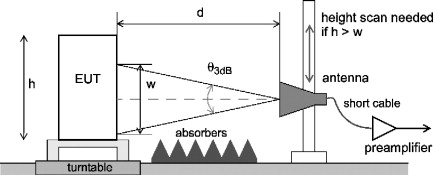
It requires a minimum value of w over the frequency range 1 to 18 GHz, which in turn implies careful selection of antenna type and measurement distance; and if the EUT' height is larger than w then it has to be scanned in height in order to cover the whole height of the EUT. A width scan is not needed as the EUT will be rotated on its turntable to find the maximum emission in azimuth.

23.4. Military Emissions Tests

The foregoing has concentrated on emissions tests to CISPR standards. Military and aerospace methods as set out in DEF STAN 59-41 and MIL STD 461E are significantly different, to the extent that making a one-to-one comparison of the results, as is necessary if military applications are to use commercial-off-the-shelf products, is very difficult. This section briefly summarizes the most important differences.

23.4.1. Instrumentation

The measuring receiver has a different detector function and bandwidth specification. The CISPR quasi-peak and average detectors are avoided; only the peak detector is used. The bandwidths are compared in Table 23.1.

Table Comparison of DEF STAN 59-41 and CISPR bandwidths

Military frequency range	6-dB bandwidth	CISPR frequency range	6-dB bandwidth
20 Hz–1 kHz	10 Hz
1 kHz–50 kHz	100 Hz
		9 kHz–150 kHz	200 Hz
50 kHz–1 MHz	1 kHz
1 MHz–30 MHz	10 kHz*
		150 kHz–30 MHz	9 kHz
30 MHz–18 GHz	100 kHz*
		30 MHz–1GHz	120 kHz

^* Some deviations for certain applications.

23.4.2. Transducers

For conducted emissions, DEF STAN tests use a LISN on the power lines, but it is the 50-Ω/5-μH version with a frequency range from 1 kHz to 400 MHz over which the impedance is defined. It is permanently connected to the power supplies and used in all tests, not only those that measure power supply emissions. For DC supplies an additional 30,000-μF capacitor is connected between positive and negative on the power supply side of the two LISNs to improve the low-frequency performance.

For the radiated tests, all antennas are situated at a separation distance of 1 m from the closest surface of the EUT to the antenna calibration reference point. This is probably the single most important difference from the commercial tests under CISPR. To cover the extended frequency range required by the radiated emissions measurement, the antennas used for E-field tests are:

• 14 kHz–1.6 MHz (land systems), 30 MHz (air and sea systems): active or passive 41"
• vertical monopole (rod) antenna with counterpoise or ground plane
• 1.6 MHz–76 MHz (land systems): antenna as used in installed systems
• 25 MHz–300 MHz: biconical
• 200 MHz–1 GHz: log periodic
• 1 GHz–18 GHz: waveguide or double-ridged waveguide horns

23.4.3. Test Site

Radiated emission tests are all conducted in a screened room: There is no “open area” test site as such. The EUT is laid out on a ground plane bench which is bonded to the rear wall of the screened room, and the exact distances from the antenna to the bench and to the EUT are specified. The screened room itself has to comply with Part 5 of the DEF STAN, which includes the requirement for partial lining with anechoic material, and that the maximum dimensions of the room give a lowest chamber resonance not below 30 MHz. It should be demonstrated that the room' normalized site insertion loss (NSIL) is representative of free-space theoretical values: The maximum permitted tolerances are ±10 dB over the frequency range 80 to 250 MHz and ±6 dB from 250 MHz to 1 GHz. Measurements are to be made with both vertical and horizontal polarizations. The concept is similar to the CISPR ±4-dB requirement but for a single position of the antenna (no height scan), and of course the tolerances are much wider.

23.5. Measurement Uncertainty

EMC measurements are inherently less accurate than most other types of measurement. Whereas, say, temperature or voltage measurement can be refined to an accuracy expressed in parts per million, field strength measurements in particular can be in error by 10 dB or more, partly due to uncertainties in the measuring instrumentation and method and partly due to uncertainties introduced by the EUT setup. It is always wise to allow a margin of about this magnitude between your measurements and the specification limits, not only to cover measurement uncertainty but also tolerances arising in production.

23.5.1. Applying Measurement Uncertainty

UKAS, the body that accredits U.K. EMC test houses, issues guidelines on determining measurement uncertainty in LAB 34 (UKAS, 2002), and it requires test houses to calculate and if necessary to report their own uncertainties, but for EMC tests it does not define acceptable levels of uncertainty. Among other things this document suggests that, if there is no other specification criterion, guidance, or code of practice, test houses express their results in one of four ways, as shown in Table 23.2.

Table 23.2. Statements of compliance with specification

The product complies	The measured result is below the specification limit by a margin less than the measurement uncertainty; it is not therefore possible to determine compliance at a level of confidence of 95%. However, the measured result indicates a higher probability that the product tested complies with the specification limit.	The measured result is above the specification limit by a margin less than the measurement uncertainty; it is not therefore possible to determine compliance at a level of confidence of 95%. However, the measured result indicates a higher probability that the product tested does not comply with the specification limit.	The product does not comply

Note:

Cases B and C in the table, while being metrologically sound, are clearly not helpful to manufacturers who want a simple statement of pass or fail. However, CISPR 16-4-2 (“Uncertainty in EMC Measurements”) (CISPR, 2003) prescribes that for emissions tests the measurement uncertainty should be taken into account in determining compliance. But it goes on to give a total uncertainty figure U^CISPR for each of the principal emissions tests (Table 23.3), based only on the instrumentation and test method errors and not taking into account any contribution from the EUT. If the test house' declared uncertainty is less than or equal to this value, then direct comparison with the limit is acceptable (cases A and D with an effective measurement uncertainty of zero). If the uncertainty is greater, then the test result must be increased by the excess before comparison with the limit—effectively penalizing manufacturers who use test houses with large uncertainties.

Table 23.3. CISPR uncertainties according to CISPR 16-4-2

Measurement	UCISPR
Conducted disturbance, mains port, 9–150 kHz	4.0 dB
Conducted disturbance, mains port, 150 kHz–30 MHz	3.6 dB
Disturbance power, 30–300 MHz	4.5 dB
Radiated disturbance, 30–300 MHz	5.1 dB

23.5.2. Sources of Uncertainty

This section discusses how measurement uncertainties arise (Figure 23.4).

Figure 23.4. Sources of error in radiated emissions tests.

23.5.2.1. Instrument and Cable Errors

Modern self-calibrating test equipment can hold the uncertainty of measurement at the instrument input to within ±1 dB. To fully account for the receiver errors, its pulse amplitude response, variation with pulse repetition rate, sine-wave voltage accuracy, noise floor, and reading resolution should all be considered. Input attenuator, frequency response, filter bandwidth, and reference level parameters all drift with temperature and time and can account for a cumulative error of up to 5 dB at the input even of high-quality instrumentation. To overcome this a calibrating function is provided. When this is invoked, absolute errors, switching errors, and linearity are measured using an in-built calibration generator and a calibration factor is computed that then corrects the measured and displayed levels. It is left up to the operator when to select calibration, and this should normally be done before each measurement sweep. Do not invoke it until the instrument has warmed up—typically 30 min to an hour—or calibration will be performed on a “moving target.” A good habit is to switch the instruments on first thing in the morning and calibrate them just before use.

The attenuation introduced by the cable to the input of the measuring instrument can be characterized over frequency and for good-quality cable is constant and low, although long cables subject to large temperature swings can cause some variations. Uncertainty from this source should be accounted for but is normally not a major contributor. The connector can introduce unexpected frequency-dependent losses; the conventional BNC connector is particularly poor in this respect, and you should perform all measurements whose accuracy is critical with cables terminated in N-type connectors, properly tightened (and not cross-threaded) against the mating socket.

Mismatch Uncertainty

When the cable impedance, nominally 50Ω, is coupled to an impedance that is other than a resistive 50Ω at either end, it is said to be mismatched. A mismatched termination will result in reflected signals and the creation of standing waves on the cable. Both the measuring instrument input and the antenna will suffer from a degree of mismatch which varies with frequency and is specified as a voltage/standing-wave ratio (VSWR). If either the source or the load end of the cable is perfectly matched, then no errors are introduced, but otherwise a mismatch error is created. Part of this is accounted for when the measuring instrument or antenna is calibrated. But calibration cannot eliminate the error introduced by the phase difference along the cable between source and load, and this leaves an uncertainty component whose limits are given by (23.3)

where Γ^L and Γ^S are the source and load reflection coefficients.

As an example, an input VSWR of 1.5:1 and an antenna VSWR of 4:1 gives a mismatch uncertainty of ±1 dB. The biconical in particular can have a VSWR exceeding 15:1 at the extreme low-frequency end of its range. When the best accuracy is needed, minimize the mismatch error by including an attenuator pad of 6 or 10 dB in series with one or both ends of the cable, at the expense of measurement sensitivity.

23.5.2.2. Conducted Test Factors

Mains conducted emission tests use a LISN/AMN as described in Section 22.2.2.1. Uncertainties attributed to this method include the quality of grounding of the LISN to the ground plane, the variations in distances around the EUT, and inaccuracies in the LISN parameters. Although a LISN theoretically has an attenuation of nearly 0 dB across most of the frequency range, in practice this cannot be assumed particularly at the frequency extremes and you should include a voltage division factor derived from the network's calibration certificate. In some designs, the attenuation at extremes of the frequency range can reach several decibels. Mismatch errors, and errors in the impedance specification, should also be considered.

Other conducted tests use a telecom line ISN instead of a LISN or use a current probe to measure common mode current. An ISN will have the same contributions as the LISN with the addition of possible errors in the LCL (see Section 22.2.2.4). A current probe measurement will have extra errors due to stray coupling of the probe with the cable under test, and termination of the cable under test, as well as calibration of the probe factor.

23.5.2.3. Antenna Calibration

One method of calibrating an antenna is against a reference standard antenna, normally a tuned dipole on an open area test site (Alexander, 1989). This introduces its own uncertainty, due to the imperfections both of the test site and of the standard antenna – ±0.5 dB is now achievable—into the values of the antenna factors that are offered as calibration data. An alternative method of calibration known as the standard site method (Smith, 1982) uses three antennas and eliminates errors due to the standard antenna, but still depends on a high-quality site.

Further, the physical conditions of each measurement, particularly the proximity of conductors such as the antenna cable, can affect the antenna calibration. These factors are worst at the low-frequency end of the biconical's range and are exaggerated by antennas that exhibit poor balance (Alexander, 1985). When the antenna is in vertical polarization and close to the ground plane, any antenna imbalance interacts with the cable and distorts its response. Also, proximity to the ground plane in horizontal polarization can affect the antenna's source impedance and hence its antenna factor. Varying the antenna height above the ground plane can introduce a height-related uncertainty in antenna calibration of up to 2 dB (DeMarinis, 1989).

These problems are less for the log periodic at UHF because nearby objects are normally out of the antenna's near field and do not affect its performance, and the directivity of the log periodic reduces the amplitude of off-axis signals. On the other hand the smaller wavelengths mean that minor physical damage, such as a bent element, has a proportionally greater effect. Also the phase center (the location of the active part of the antenna) changes with frequency, introducing a distance error, and since at the extreme of the height scan the EUT is not on the boresight of the antenna, its directivity introduces another error. Both of these effects are greatest at 3-m distance. An overall uncertainty of ±4 dB to allow for antenna-related variations is not unreasonable, although this can be improved with care.

The difficulties involved in defining an acceptable and universal calibration method for antennas that will be used for emissions testing led to the formation of a CISPR/A working group to draft such a method. It has standardized on a free-space antenna factor determined by a fixed-height three-antenna method on a validated calibration test site (Goedbloed, 1995). The method is fully described in CISPR 16-1-5.

23.5.2.4. Reflections and Site Imperfections

The antenna measures not only the direct signal from the EUT but also any signals that are reflected from conducting objects such as the ground plane and the antenna cable. The field vectors from each of these contributions add at the antenna. This can result in an enhancement approaching +6 dB or a null that could exceed −20 dB. It is for this reason that the height scan referred to in Section 23.2 is carried out; reflections from the ground plane cannot be avoided but nulls can be eliminated by varying the relative distances of the direct and reflected paths. Other objects further away than the defined CISPR ellipse will also add their reflection contribution, which will normally be small (typically less than 1 dB) because of their distance and presumed low reflectivity.

This contribution may become significant if the objects are mobile, for instance people and cars, or if the reflectivity varies, for example trees or building surfaces after a fall of rain. They are also more significant with vertical polarization, since the majority of reflecting objects are predominantly vertically polarized. With respect to the site attenuation criterion of ±4 dB, CISPR 16-4-2 states: “measurement uncertainty associated with the CISPR 16-1 site attenuation measurement method is usually large, and dominated by the two antenna factor uncertainties. Therefore a site which meets the 4 dB tolerance is unlikely to have imperfections sufficient to cause errors of 4 dB in disturbance measurements. In recognition of this, a triangular probability distribution is assumed for the correction δSA” (CISPR, 2003, clause A.5).

Antenna Cable

With a poorly balanced antenna, the antenna cable is a primary source of error (DeMarinis, 1988, 1989). By its nature it is a reflector of variable and relatively uncontrolled geometry close to the antenna. There is also a problem caused by secondary reception of common-mode currents flowing on the sheath of the cable. Both of these factors are worse with vertical polarization, since the cable invariably hangs down behind the antenna in the vertical plane. They can both be minimized by choking the outside of the cable with ferrite sleeve suppressors spaced along it or by using ferrite loaded RF cable. If this is not done, measurement errors of up to 5 dB can be experienced due to cable movement with vertical polarization. However, modern antennas with good balance, which is related to balun design, will minimize this problem.

23.5.2.5. The Measurement Uncertainty Budget

Some or all of the preceding factors are combined together into a budget for the total measurement uncertainty that can be attributed to a particular method. The detail of how to develop an uncertainty budget is beyond the scope of this book, but you can refer to LAB 34 (UKAS, 2002) or CISPR 16-4-2 (CISPR, 2003) for this. Essentially, each contribution is assigned a value and a probability distribution. These are derived either from existing evidence (such as a calibration certificate) or from estimation based on experience, experiment, or published information. Contributions can be classified into two types: Type A contributions are random effects that give errors that vary in an unpredictable way while the measurement is being made or repeated under the same conditions. Type B contributions arise from systematic effects that remain constant while the measurement is made but can change if the measurement conditions, method, or equipment is altered.

The “standard uncertainty” for each contribution is obtained by dividing the contribution's value by a factor appropriate to its probability distribution. Then the “combined standard uncertainty” is given by adding the standard uncertainties on a root-sum-of-squares basis; and the “expanded uncertainty” of the method, defining an interval about the measured value that will encompass the true value with a specified degree of confidence and which is reported by the laboratory along with its results, is calculated by multiplying the combined standard uncertainty by a “coverage factor” k. In most cases, k = 2 gives a 95% level of confidence.

A simplified example budget for a straightforward conducted emissions test is given in Table 23.4. This is derived from LAB 34 (UKAS, 2002); the contributions are typical values, but each test lab should derive and justify its own values to arrive at its own overall uncertainty for the test. Each measurement method (conducted emissions, radiated emissions, disturbance power) needs to have its own budget created, and it is reasonable to subdivide budgets into, for example, frequency subranges when the contributions vary significantly over the whole range, such as with different antennas.

Table 23.4. Example uncertainty budget for conducted measurement 150 kHz to 30 MHz

Contribution	Value	Prob. dist.	Divisor	ui (y)	ui (y)∧2
Receiver sine-wave accuracy	1.00	Rectangular	1.732	0.577	0.333
Receiver pulse amplitude response	1.50	Rectangular	1.732	0.866	0.750
Receiver pulse repetition response	1.50	Rectangular	1.732	0.866	0.750
Receiver indication	0.05	Rectangular	1.732	0.029	0.001
Frequency step error	0.00	Rectangular	1.732	0.000	0.000
Noise floor proximity	0.00	Rectangular	1.732	0.000	0.000
LISN attenuation factor calibration	0.20	Normal, k = 2	2.000	0.100	0.010
Cable loss calibration	0.40	Normal, k = 2	2.000	0.200	0.040
LISN impedance	2.70	Triangular	2.449	1.102	1.215
Mismatch	−0.891	U-shaped	1.414	−0.630	0.397
Receiver VRC	0.15
LISN + cable VRC	0.65
Measurement system repeatability	0.50	Normal, k = 1	1.000	0.500	0.250
Combined standard uncertainty	Normal			1.936	3.746
Expanded uncertainty		Normal, k = 2.0		3.87

Entered = 0.15

Calculated = 0.5

Result = 3.87

It is important to realize that this is, strictly speaking, a measurement instrumentation and method uncertainty budget. It does not take into account any uncertainty contributions attributable to the EUT itself or to its setup, because the lab cannot know what these contributions are, yet they are likely to be at least as important in determining the outcome of the test as the visible and calculable contributions.

23.5.2.6. Human and Environmental Factors

The Test Engineer

It should be clear from Section 23.4 that there are many ways to arrange even the simplest EUT to make a set of emissions measurements. Equally, there are many ways in which the measurement equipment can be operated and its results interpreted, even to perform measurements to a well-defined standard—and not all standards are well defined. In addition, the quantity being measured is either an RF voltage or an electromagnetic field strength, both of which are unstable and consist of complex waveforms varying erratically in amplitude and time. Although software can be written to automate some aspects of the measurement process, still there is a major burden on the experience and capabilities of the person actually doing the tests.

Some work has been reported that assesses the uncertainty associated with the actual engineer performing radiated emission measurements (Robinson, 1989). Each of four engineers was asked to evaluate the emissions from a desktop computer consisting of a processor, VDU, and keyboard. This remained constant although its disposition was left up to the engineer. The resultant spread of measurements at various frequencies and for both horizontal and vertical polarization was between 2 and 15 dB—which does not generate confidence in their validity! Two areas were recognized as causing this spread, namely differences in EUT and cable configurations and different exercising methods.

The tests were repeated using the same EUT, test site, and test equipment but with the EUT arrangement now specified and with a fixed antenna height. The spread was reduced to between 2 and 9 dB, still an unacceptably large range. Further sources of variance were that maximum emissions were found at different EUT orientations, and the exercising routines still had minor differences. The selected measurement time (Section 22.1.3.4) can also have an effect on the reading, as can ancillary settings on the test receiver and the orientation of the measurement antenna.

Ambients

The major uncertainty introduced into EMC emissions measurements by the external environment, apart from those discussed already, is due to ambient signals. These are signals from other transmitters or unintentional emitters such as industrial machinery, which mask the signals emitted by the EUT. On an open-area test site (OATS), they cannot be avoided, except by initially choosing a site that is far from such sources. In a densely populated country such as the United Kingdom, and indeed much of Europe, this is wishful thinking. A “greenfield” site away from industrial areas, apart from access problems, almost invariably falls foul of planning constraints, which do not permit the development of such sites—even if they can be found—for industrial purposes.

Another Catch-22 situation arises with regard to broadcast signals. It is important to be able to measure EUT emissions within the Band II FM and Bands IV and V TV broadcast bands since these are the very services that the emission standards are meant to protect. But the raison d'être of the broadcasting authorities is to ensure adequate field strengths for radio reception throughout the country. The BBC publishes its requirements for the minimum field strength in each band that is deemed to provide coverage (BBC, 1990/1991) and these are summarized in Table 23.5. In each case, these are (naturally) significantly higher than the limit levels that an EUT is required to meet. In other words, assuming countrywide broadcast coverage is a fact, nowhere will it be possible to measure EUT emissions on an OATS at all frequencies throughout the broadcast bands because these emissions will be masked by the broadcast signals themselves.

Table 23.5. Minimum broadcast field strengths in the United Kingdom

Service	Frequency range	Minimum acceptable field strength
Long wave	148.5–283.5 kHz	5 mV/m
Medium wave	526.5–1606.5 kHz	2 mV/m
VHF/FM band II	87.5–108 MHz	54 dBµV/m
TV band IV	471.25–581.25 MHz	64 dBµV/m
TV band V	615.25–853.25 MHz	70 dBµV/m

[source]Source: BBC, 1990/1991.

Source: BBC, 1990/1991.

The only sure way around the problem of ambients is to perform the tests inside a screened chamber, which is straightforward for conducted measurements but for radiated measurements is subject to severe inaccuracies introduced by reflections from the wall of the chamber as discussed earlier. An anechoic chamber will reduce these inaccuracies and requirements for anechoic chambers are now in the standards, as mentioned in Section 22.3.1.3, but a fully compliant anechoic chamber will be prohibitively expensive for many companies. (Major blue-chip electronics companies have indeed invested millions in setting up such facilities in-house.) The method of prescan in a nonanechoic chamber discussed in Section 23.2 goes some way toward dealing with the problem, but does not solve the basic difficulty that a signal that is underneath an ambient on an OATS cannot be accurately measured.

Emissions standards such as EN 55022 recognize the problem of ambient signals and in general require that the test site ambients should not exceed the limits. When they do, the standard allows testing at a closer distance such that the limit level is increased by the ratio of the specified distance to the actual distance. This is usually only practical in areas of low signal strength where the ambients are only a few decibels above the limits. Some relief can be gained by orienting the site so that the local transmitters are at right angles to the test range, taking advantage of the antennas' directional response at least with horizontal polarization.

When you are doing diagnostic tests the problem of continuous ambients is less severe because, even if they mask some of the emissions, you will know where they are and can tag them on the spectrum display. Some analysis software performs this task automatically. Even so, the presence of a “forest” of signals on a spectrum plot confuses the issue and can be unnerving to the uninitiated. Transient ambients, such as from portable transmitters or occasional broadband sources, are more troublesome because it is harder to separate them unambiguously from the EUT emissions. Sometimes you will need to perform more than one measurement sweep in order to eliminate all the ambients from the analysis.

Ambient Discrimination by Bandwidth and Detector

Annex A to CISPR 16-2-3 (CISPR, 2006) attempts to address the problem of ambients from another angle. This distinguishes between broadband and narrowband EUT emissions in the presence of broadband or narrowband ambient noise (Figure 23.5). If both the ambient noise and the EUT emissions are narrowband, a suitably narrow measurement bandwidth is recommended, with use of the peak detector. The measurement bandwidth should not be so low as to suppress the modulation spectra of the EUT emission. If the EUT noise is broadband, the measurement cannot be made directly underneath a narrowband ambient but can be taken either side, and the expected actual level interpolated.

Figure 23.5. Ambient discrimination on the basis of bandwidth.

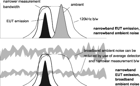
When the ambient disturbance is broadband, bandwidth discrimination is not possible, but a narrowband EUT emission may be extracted by using the average detector with a narrower measuring bandwidth that maximizes the EUT disturbance-to-ambient ratio. The average detector should reduce the broadband level without affecting the desired EUT narrowband signal, as long as the EUT signal is not severely amplitude or pulse modulated; if it is, some error will result.

Broadband EUT disturbances in the presence of broadband ambients cannot be directly measured, although if their levels are similar (say, within 10 dB) it is possible to estimate the EUT emission through superposition, using the peak detector.

References

Alexander, 1989 M.J. Alexander, NPL EMC Antenna Calibration and the Design of an Open Space Antenna Range British Electromagnetic Measurements Conference, Teddington, UK, November 7–9, 1989 1989

Alexander, 1995 M.J. Alexander, NPL Antenna Related Uncertainties in Screened Room Emission Measurements IEE Colloquium on EMC Tests in Screened Rooms, April 11, 1995, IEE Colloquium Digest 1995/074 1995

BBC, 1990/1991 BBCBBC Radio Transmitting Stations 1991. BBC Television Transmitting Stations 1990 BBC Engineering Information 1990/1991 BBC White City, London

CISPR, 2003 CISPR CISPR 16-4-2:2003 Specification for Radio Disturbance and Immunity Measuring Apparatus and Methods: Part 4-2: Uncertainties, Statistics and Limit Modelling—Uncertainty in EMC Measurements 2003

CISPR, 2005 CISPR CISPR 22 Ed. 5 A1: 2005: Information Technology Equipment—Radio Disturbance Characteristics—Limits and Methods of Measurement Amendment 1: Emission Limits and Method of Measurement from 1 GHz to 6 GHz 2005

CISPR, 2006 CISPR CISPR 16-2-3 Ed.2: 2006 Specification for Radio Disturbance and Immunity Measuring Apparatus and Methods—Part 2-3: Methods of Measurement of Disturbances and Immunity—Radiated Disturbance Measurements 2006

DeMarinis, 1988 J. DeMarinis, DEC The Antenna Cable as a Source of Error in EMI Measurements International Symposium on EMC, IEEE, Washington, DC, August 2–4, 1988 1988

DeMarinis, 1989 J. DeMarinis, DEC Getting Better Results from an Open Area Test Site Eighth Symposium on EMC, Zurich, Switzerland, March 1989 1989

Goedbloed, 1995 J.J. Goedbloed, Philips Research Progress in Standardization of CISPR Antenna Calibration Procedures 11th International Symposium on EMC, Zurich, Switzerland, March 7–9, 1995 1995

Robinson, 1989 M.F. Robinson, British Telecom EMC Measurement Uncertainties British Electromagnetic Measurements Conference, Teddington, UK, November 7–9, 1989 1989

Smith, 1982 A.A. Smith, IBM Standard Site Method for Determining Antenna Factors IEEE Transactions on Electromagnetic Compatibility EMC-24, no. 3 (August) 1982

UKAS, 2002 UKAS The Expression of Uncertainty in EMC Testing UKAS Publication LAB 34, Feltham, UK Edition 1 2002 available at www.ukas.com