Chapter 26. HALT and FMVT

Highly accelerated life testing (HALT) is a test method, with its very imprecise acronym (it does not measure “life,” and there is no quantification of what highly means) has been used, abused, lauded and ridiculed, written, and documented for many years. This chapter will discuss what the test method is supposed to do, guidance and examples of accomplishing the test properly with references to scholarly work on doing it right. Also included are examples of how to really “mess it up.”

“How much wood would a woodchuck chuck if a woodchuck could chuck wood?”

The HALT process would be a good tool to determine the answer to this tongue-twister riddle. The basic principle of highly accelerated life testing is the margin discovery process. The goal of this process is to determine the margins between the service conditions of the product and the functional limits and the destruct limits. In other words, how much wood would the woodchuck chuck, or how much temperature can the circuit board handle, or how much vibration, or how cold, or how much voltage.

HALT is a test method usually applied to solid-state electronics that determines failure modes, operational limits, and destruct limits. This test method differs significantly from reliability tests. HALT does not determine a statistical reliability or (despite its acronym) determine an estimated life. HALT applies one stress source at a time to a product at elevated levels to determine the levels at which the product stops functioning but is not destroyed (operational limit), the levels at which the product is destroyed (destruct limit) and what failure modes cause the destruction of the product.

HALT has a significant advantage over traditional reliability tests in identifying failure modes in a very short period of time. Traditional reliability tests take a long period of time (from a few days to several months). A HALT typically takes two or three days. Also, a HALT will identify several failure modes providing significant information for the design engineers to improve the product. Typical reliability tests will provide one or two failure modes, if the product fails at all.

HALT typically uses three stress sources: temperature, vibration, and electrical power. Each stress source is applied starting at some nominal level (for example, 30° C) and is then elevated in increments until the product stops functioning. The product is then brought back to the nominal conditions to see if the product is functional. If the product is still functional, then the level at which the product stopped functioning is labeled the operational limit. The product is then subjected to levels of stress above the operational limit, returning to nominal levels each time until the product does not function. The maximum level the product experienced before failing to operate at nominal conditions is labeled the destruct limit. This process is repeated for hot temperature, cold temperature, temperature ramp rate, vibration, and voltage. The process is also repeated for combined stress.

There are two significant disadvantages to HALT. Without a statistical reliability measure, the method does not fit well into the requirements for contracting between suppliers and purchasers. This relationship requires an objective measure that can be written into a contract. Some schemes have been suggested that would allow the objective measure of the relationship between the “operational limit” of the product and the service conditions. The second disadvantage to HALT is the amount of time the test method can take to address a significant number of stress sources. Each stress source tested requires about one day of testing and one or two sample products. Since HALT is usually applied to solid-state electronics, the stress sources are limited to hot, cold, ramp, vibration, and voltage. This requires six parts (including the combined environment test) and four or five days (8-hr days). However, applying the method to 10 or 20 stress sources increases the number of parts to 11 or 21, respectively, and the days of testing to 10 or 20, respectively.

26.1. A Typical HALT

26.1.1. Fixturing and Operation

Because the HALT margin discovery process is based on determining at what stress level the product stops working, it is important that the product be fixtured and instrumented to provide for quick and thorough performance evaluation. The instrumentation needed for a conventional fully censored test is usually far more Spartan than for a step stress, HALT, or FMVT. With a conventional fully censored test, it is assumed that the product is going to survive for the whole test period. The only piece of information that is relevant is whether the product is working at the end of the test. For this reason, the instrumentation during the test may be very simple or even nonexistent on the fully censored reliability test. With the HALT process, the goal is to determine exactly when and how the product fails.

Proper instrumentation must follow from a proper definition of what a failure is for the product and what the effects of the failure are. Using the failure mode effects analysis can be a good source for the definition of the failure modes and equally important their effects (Porter, 1999).

When determining the instrumentation for the failures, the effects of the failure are often the key to properly checking the instrument for the existence of the failure. For example, a sealed bearing has the potential failure of galling. With a sealed bearing, it is very difficult to determine the existence of galling on the sealed bearing surface. In a conventional fully censored reliability test, the part could be cut open at the end of the test. During a HALT, a less invasive way of determining when the failure occurs (and progresses) is needed. In the case of a sealed bearing, the effect of galling on the bearing performance in the system would be a logical choice. A sealed bearing in a hard drive can be instrumented for galling by monitoring the current. Since hard drive motors turn at a constant rpm, the current draw will increase if the bearing galls.

Table 26.1 shows some other examples of failure modes, their effect, and the instrumentation.

Table 26.1. Device failure

Failure mode	Effect	Instrumentation
Bearing galling in hard drive	Increased current draw	Current measurement (and voltage)
Cracked substructure in complex plastic assembly	Shift in natural frequency of assembly	Accelerometer at antinode
Seal leak in pneumatically sealed enclosure for ABS brake system	Moisture ingress into sensitive electrohydraulics	Precharge enclosure with halogen gas—use halogen detector to monitor for leaks

Notice that instrumentation of this kind requires an understanding of the whole product, not just the individual failure mode. For example, the cracked substructure in a complex plastic assembly can be detected by placing an accelerometer at the antinode of the product. An antinode is a place on a product that moves the most while under vibration (a node is a place that does not move while under vibration). Imagine a string that is attached at one end to a wall and you move the other end up and down. Move it at one speed and you will get one “wave” in the string, move it faster and you can get two waves. With two waves, the two “peaks” are the antinodes, moving the most. The point in the middle of the string that does not move is the node. (See Figure 26.1.)

Figure 26.1. Node and antinode illustration. The node is the point on a product (in this case, a string) that does not move due to the natural resonance of the product. It is worth noting that the antinode of the first mode shape (left) is a node for the second mode shape.

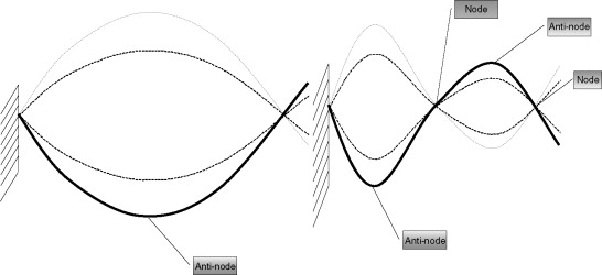
When the part begins to crack, the stiffness of the product will change and the natural frequency will drop.

Where

In order to use an accelerometer to detect a crack in this manner, it is important to know where the antinode is. This requires either a resonance survey or the use of a finite element analysis (FEA) to determine the mode shapes (the shape a product takes under vibration).

If the accelerometer is not put at the antinode, a crack could develop and not be detected. The reality is that every product has multiple mode shapes and the major mode shapes have to be considered to determine points at which the accelerometer can be placed so that it does not sit near a node and as close as possible to an antinode. If the accelerometer sits on a node, then there is no motion from that mode shape, and detecting a change in the mode shape due to a stiffness change will be very difficult.

Once the instrumentation is determined then the testing can start.

26.2. Hot Temperature Steps

During the temperature steps, a decision must be made whether to control the ambient temperature or the part temperature. The ambient temperature is often used, since this temperature will be the easiest to correlate to the final field conditions. However, when electronic component testing is being conducted, the part temperature is used.

Why? For an assembled product like an automotive audio amplifier, the ambient service conditions are fairly well defined. The part temperatures will be a direct function of those ambient conditions and the thermal dynamic properties of the packaging and power dissipation. In this case, the ambient conditions are what matter; the part temperature will be what it will be. In the case of component testing (a capacitor, for example), the part temperature is used because the final ambient conditions of the package the capacitor will go in is not known. In fact, a given capacitor model will most likely find itself in a wide range of packages and resulting ambient conditions. The capacitor manufacturer is therefore interested in rating the capacitor for its maximum part temperature, which will be higher than the ambient temperature of the amplifier.

During the hot temperature steps, the product is held at either an ambient temperature or a part temperature (assembly or component, respectively) until the part temperature stabilizes.

Once the product stabilizes (either at the target component temperature or at a stable temperature in the target ambient temperature), the functionality of the product is checked. Note: This is a key point for making an efficient HALT test—make the performance checks fast but thorough. It is a common mistake to plan for the time it takes to reach temperature and not plan for efficient performance evaluation. I have seen this lead to 10 days to execute a planned 2-day test because the performance tests were not planned out properly.

When the product fails the performance testing, the temperature is dropped back down to the nominal service conditions and the part is allowed to stabilize. The performance checks are rerun to determine if the part recovered. If the part does recover, then the “operational limit” has been discovered. If the part does not recover, then the “destruct limit” has been discovered (Hobbs, 2000). The operational limit often exists for electronic components and some electromagnetic devices like motors and solenoids. Many mechanical devices will not have an operational limit (temperature at which they stop working but recover if cooled) but will simply operate until they reach a temperature that destroys them. Some purely mechanical devices will function to temperatures well above what can be tested in a standard chamber (which can go to between 177° C to 200° C).

Once the operational limit has been determined, the test gets slower. The product must be brought to ever higher temperatures (at which it will not work) and then returned to nominal service conditions until a temperature is found that destroys the product (no recovery when returned to nominal temperatures). (See Figure 26.2.) This process can take a very long time. Using a couple of extra samples can speed up the process. Establish the operational limit, then increase the temperature to a much higher temperature (for example, 50° C) and check if the part has been destroyed. If not, go another 50° C. Once the part reaches a 50° C increment that destroys the product, use another sample and try 25° C cooler. Continue to halve the temperature until the destruct limit is known. (See Figure 26.3.)

Figure 26.2. Margin discovery process.

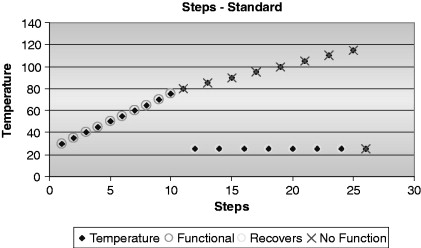
Figure 26.3. Margin discovery process using a binary search.

26.3. Cold Temperature Steps

Cold temperature steps are accomplished in a similar way to the hot temperature steps. Aside from the obvious change (going colder instead of hotter, from the coldest nominal services condition instead of the hottest), a couple of other factors should be kept in mind. It is more likely that the limits of the chamber will be reached before an operational limit or destruct limit is reached, especially with motors, amplifiers, and other devices that create their own heat. With these types of devices, two types of test may be necessary: continuous operation and duty cycling.

With continuous operation, the unit is powered and loaded while being cooled. This allows the unit to maintain some of its own internal temperature. Just like people out in the cold can keep warm if they keep moving—products that function continuously while being cooled are more likely to survive. Duty cycling the product by shutting it off—letting it cool until it has stabilized and then trying to start it up again—is a harsher test. It also takes much longer, especially for larger products. One, or the other, or both methods can be chosen based on the information needs of the project. A product like an audio amplifier that must start up on a cold winter day after sitting would benefit from the duty cycle method, while a telephone switching box that will be in an unheated shed may use the continuous method.

Because the unit may very well function all the way down to the limits of the chamber, it may be a good idea to check that temperature first, noting that if the coldest temperature destroys the part, then the sample size for the test must be increased by one. On the other hand, if it is discovered that the product survives at the coldest temperatures, then a day or two of testing is avoided.

26.4. Ramp Rates

Once the hot and cold operational and destruct limits are discovered, then the effect of thermal ramp rates can be determined. If both an upper and lower operational and destruct limit have been discovered, then a decision must be made whether to ramp between the service limits or operational limits. If there are no operational limits, avoid using the destruct limits. The purpose of the ramp portion of the test is to determine the ramp rate at which thermal expansion differences in the materials cause a failure. If the product is taken too close to the destruct limits, then the failures may not be due to the ramp effect.

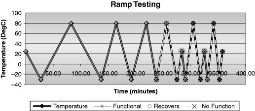
Once two temperatures have been chosen to ramp between, the product is heated and cooled at a mild ramp rate while checking its functionality. Once the product has been ramped up and down at a given ramp rate without failure, the ramp rate is increased. The process is continued until the unit no longer functions. The unit is returned to nominal operating temperatures and is functionally checked again. If the unit functions, then the ramp rate is increased again. (See Figure 26.4.)

Figure 26.4. Ramp testing.

Note that ramp rates often make a bigger difference on electronic products and some functional items that are highly susceptible to the effects of different coefficients of linear thermal expansion in the materials that make up the product. The fast ramp rates causes the parts on the outer surfaces to achieve different temperatures than parts inside the product. (See Figure 26.5.)

Figure 26.5. Ramp rate and direction are both important to thermal stress.

26.5. Vibration

The vibration portion of the test is critical. Vibration is prevalent in nearly every product environment. Even a paper towel dispenser mounted on a bathroom wall sees vibration. Technically, the only environment that is devoid of vibration would be absolute zero. Everything else is vibrating.

Vibration is a very nonintuitive stress source. So let us take a little time to look at it.

Vibration is usually measured as an acceleration amplitude (distance per unit time squared such as m/s² or ft/s²) vs. frequency. Gravity is the most prevalent form of acceleration (9.81 m/s²) and is the subject of many high school physics questions involving throwing a ball. But vibration does not go in one direction like gravity, which pulls you towards the center of the Earth, Mars, or Venus (depending on where you live). Acceleration in vibration oscillates at some rate. In fact, random vibration can cause acceleration oscillations at many rates at the same time (Holman, 1994). Just like white light has a full spectrum (wavelength) of light in it, random vibration has a wide range of vibration rates. This is an important concept to grasp for proper testing using vibration. Random vibration is not a series of discreet oscillations at different rates; it is all the rates in the spectrum at the same time. When white light is passed through a prism and is separated into its separate colors, you do not see the colors pulse or alternate as different frequencies (wavelengths) of light pass through the prism, averaging white light. They are all present at the same time.

Understanding that random vibration is a spectrum of oscillation rates or a frequency spectrum leads to a logical question. What is the frequency range? Visible light has a known wavelength range, with infrared and ultraviolet beyond the visible range. Vibration has frequency ranges also. A swing on a playground oscillates at less then 1 Hz (it takes longer than 1 s to swing back and forth), while the surface-mounted chip inside your computer has a mechanical resonance (oscillation) as high as 10,000 Hz.

Now consider the swing on the playground for a moment. To make it swing requires an input energy in the form of some type of periodic or oscillating energy source. In most cases, this is the swinger kicking his or her legs forward while they leaning back followed by kicking those legs back while leaning forward. The other method is for someone (would this be the swingee?) to push the swinger periodically. If you have ever swung on a swing you know that you must put the energy in at the correct rate, in pace with the swing of the swing. If you try to push the swing at different times then you will not swing very far. This is critical to understanding the function of vibration in breaking a part!

What? Why?

Because, breaking a device under test requires generating strain in the product. Strain is displacement in the structure. When a structure oscillates under the vibration input, it experiences strain. The amount of strain is directly related to the amplitude of the acceleration and to how well the input oscillation matches the natural oscillation of the part. Just like the swing, if you do not put the energy in at the right pace or beat, then much less strain will take place (see Figures 26.6 and 26.7). The only real difference is that swings swing at a very low frequency and most products that we want to test oscillate at much higher frequencies. The higher frequencies contribute to the nonintuitive nature of the vibration, above about 50 Hz or so you can rarely see the motion. Thus the frequency range is important.

Figure 26.6. Pushing a swing at the correct rate or pace will result in the greatest amplitude.

Figure 26.7. Pushing the swing at the wrong time will actually slow the swing down.

Traditionally, HALT testing has used an air hammer table. There are various forms of these devices in existence. The basic premise is to have several pneumatic hammers repeatedly beating on the underside of a table to induce the table to resonate and generate random vibration on the top side of the table. This type of vibration is sometimes called repeated shock or pseudo random. These tables have been used because they can produce very high-frequency ranges suitable for solid-state electronics.

During the vibration stage, the product is subjected to vibration at ever-increasing levels until the unit stops functioning. If the unit recovers once vibration is removed, then the operational limit has been found. Vibration is then increased to find the destruct limit (energy level at which the unit stops functioning and does not recover). This process is much faster for vibration than for the hot or cold portions of the test because vibration takes only a few milliseconds to stabilize. (See Figure 26.8.)

Figure 26.8. Air hammer tables (repetitive shock) (Envirotronics Star44).

26.6. Combined Run

Once the upper and lower operational and destruct limits have been established for temperature and the operational and destruct limits for ramp and vibration, a combined run is conducted to see if there are any failure modes that require a combination of temperature, ramp, and vibration to induce failure.

26.7. Business Structures

HALT testing in the supply chain has some benefits and drawbacks. For the innovative company that is interested in understanding the functional limits of its product (under what conditions will it work), the test is extremely useful. That is to say that, if the functional limits of the product is data that will affect the behavior of a sentient being, then the test is useful.

For the commodity supplier in the supply chain, there is a problem. The test finds margins and failure modes, but does not quantify how long the part will last before the failures are experienced in the field. This means the results are not useful for the contractual reliability demonstrations often required in the relationship between a purchaser and a supplier.

Manufacturers of commodity items at the component level (such as resistors and capacitors) find the test useful for determining the operational limits of their product and to determine the failure mode when it does fail. Being able to publish this information can be helpful.

When applied to design validation HALT works well, but the process is too long for production screening. HALT applied to production screening requires a slight modification. Often called highly accelerated stress screening (HASS), the production screening based on HALT uses a narrow set of conditions to precipitate failures in bad parts while leaving good parts alone. In this method, 100% of the product is screened. Alternatively, a sampled screen in which a few parts from each lot are tested to failure can be used with a full HALT.

How do you choose between 100% screen and a sampled screen? This comes down to two key factors: (1) Can the screen be engineered to precipitate failures without damaging good product? (2) Is the production process controlled enough to apply statistical sampling?

These two questions are important. If a 100% screen is applied, then the screen must not damage the good parts but find the bad parts. But the statistical question is important also. It is more economical to use a sampled screen (few parts to test and a more aggressive screen can be used). But a sampled screen cannot be used unless the production process is highly repeatable. When the production process is repeatable, then a statistical screen can detect drift in the quality of production. For example, sampled screen based on HALT may be used to get the results in Table 26.2 from each lot.

Table 26.2. Example of a sampled screen based on HALT

Lot	Time to failure
9/12/03–1	126.4
9/12/03–2	127.3
9/12/03–3	125.1
9/13/03–1	123.1
9/13/03–2	121.1
9/13/03–5	101.2

You can see that the time to failure is drifting—this would indicate a drop in the quality. Obviously, with a sampled screen, the samples can be taken to failure. With a 100% screen, the samples that are good must not be damaged. This means the screen should be tested by passing a group of samples through the screen one or more times and running the full HALT on them and compare the results to a full HALT on a set of parts that have not been screened. There should be no discernable difference.

A 100% screen should be used if (1) the failures from the production process are random and a statistical test cannot predict the quality of the product or (2) the screen has been demonstrated to precipitate failures in bad product, while leaving good product undamaged.

A sampled screen should be used if the failures from the production process are statistically predictable due to drift in the process.

26.8. Failure-Mode Verification Testing

Don't be discouraged by a failure. It can be a positive experience. Failure is, in a sense, the highway to success, inasmuch as every discovery of what is false leads us to seek earnestly after what is true, and every fresh experience points out some form of error which we shall afterwards carefully avoid—John Keats

HALT was developed and predominantly applied to electronics. The following is a brief discussion of how failure-mode verification testing (FMVT) was developed out of HALT. We will discuss what the test method does, how to set up the test method, mistakes and problems to avoid, and examples.

HALT has been around since before 1979 for testing solid-state electronics (Abstein et al., 1980). Various attempts have been made to apply HALT to mechanical testing. In 1996, I traveled to Denver to the Hobbes Engineering Symposium to learn about accelerated reliability from Wayne Nelson. There, I was also introduced to the HALT process. Working predominantly in the automotive industry, I recognized that HALT had some application, but most of the products I had to test were much more mechanical or larger electrical systems instead of solid-state electronics.

Upon returning from Denver, I began to explore why HALT worked on solid-state electronics. At the time, my primary focus had been the implementation of finite element analysis in the lab setting. We had used FEA to model the parts we were testing. One of the first things I did was model a cup holder and apply single axis (one degree of freedom) stress vs. six-axis (three translations and three rotations) random stress to the computer model and looked at the resulting stress and mode shapes. It become obvious that the reason six-axis random vibration worked to uncover so many key failure modes was because it had the potential to activate all the mode shapes of the product.

Not all six-axis vibration is the same. The frequency range of the vibration matters. If the energy is not put in at the natural frequency of a particular mode shape then the energy is mostly wasted. This realization (which many other users of vibration have found; e.g., Tustin, 1969, 1978) led to the first key observation about HALT: “It is not the vibration, it is the stress.” In other words, the vibration spectrum is not an end but a means, the means of creating random stress throughout the product. If the product experiences random stress throughout, distributed based on how the geometry and function will naturally concentrate the stress, then the weakest feature will accumulate stress damage faster than the rest of the features.

Understanding that, the random stress in the product led to the first major divergence from HALT. Instead of including the typical temperature, vibration, and possibly electrical stress, a thorough test on mechanical and electromechanical designs should encompass all sources of stress that can damage the product.

At the same time that this understanding was developed and first applied to a real cup holder in a physical test (sources of damage included vibration, temperature, humidity, cycling, and cup loads), a second realization was developed. The design-failure-mode effects analysis (DFMEA) provided a good source for the long list of potential sources or mechanisms of damage to the part. Also, because the list of stresses was now getting large (often over 10n separate sources of stress), the normal process of margin discovery used in HALT was not practical. Therefore, two final developments took place: Use 10 steps with all of the stresses combined and randomized relative to each other (to keep the random stress on the product) and correlate the test to the potential failure modes in the DFMEA. These changes led to the change in test name (since it was a new test) that reflected the purpose of the test—to verify failure modes from the DFMEA-FMVT. These developments are embodied in U.S. patents: 6,035,715—method and apparatus for optimizing the design of a product; 6,233,530—control system for a failure mode testing system; 6,247,366—design maturity algorithm. Entela, Inc., holds all patents; and special thanks to Mark Smith of Entela, who is coinventor on the control system patent.

In addition to the testing practices developed over this period of time, a pneumatic six-axis vibration machine that could produce up to 4 in. of displacement and a frequency range from 5 Hz to 2500 Hz was developed. This machine (called the FMVT machine; see Figure 26.9), along with air hammer tables, single-axis machines, and a six-axis servo-hydraulic machine where used to provide the full-range of testing frequency at Entela.

Figure 26.9. Entela FMVT “pod.”

26.9. Development FMVT

Failure-mode verification testing uses multiple stresses applied to the product, starting at service conditions, and then elevated to a destruct level in a stepwise fashion. The stresses are applied in a random fashion in order to maximize the number of combinations of stress that are applied to the product. The goal of the test is to find multiple failure modes, analyze the failure mode progression, and determine the significant failure modes to be addressed to improve the product. The potential for improvement and the maturity of the design are also determined. (See Figure 26.10.)

Figure 26.10. Temperature and vibration for a typical FMVT.

In a development FMVT, the primary goals are the identification and sorting of failure modes to determine what to fix on the design to make the product more robust. FMVT drives the product toward a design where the product lasts for a long period of time and all of the damage is accumulated uniformly throughout the product. By driving this optimization, the FMVT results in a product that is as good as it can be for the given technology. The product can then be compared to existing designs and its reliability measured.

The goal of the test is to precipitate failure modes from all stress sources in an order that approximates their relevance. By applying all of the stresses simultaneously and elevating them from service conditions toward a destruct limit, the failures can be shown to be precipitated in approximately the order of relevance (Porter, 2002).

With the FMVT, the testing is conducted on a single sample. The analysis is not statistical but is designed to check two assumptions. First, that the design is capable of producing a viable product for the environments applied. Second, that a good design and fabrication of the product would last for a long period of time under all of the stresses that it is expected to see and would accumulate stress damage throughout the product in a uniform way, so that when one feature fails, the rest of the product's features are near failure. Therefore, the hypothesis of the test is this: The product will last for a long period of time under all stress conditions and will then exhibit multiple diverse failures throughout the product. (See Figure 26.11.) The hypothesis is rejected if failures occur early or if they occur isolated in time relative to the bulk of the failures. (See Figure 26.12.)

Figure 26.11. Hypothesized progression of failures.

Figure 26.12. Hypothesis rejected.

The test is set up with the level one stresses set at service conditions. If the hypothesis is correct, that the product is accumulating stress damage throughout the product in a uniform way, then at level 1 the rate of stress damage will be uniform. Level 10 of the test is set up with each stress source raise to a destruct limit or a change in the physics of failure. For example, the maximum temperature would not be raised above the glass transition point of a plastic part, and the voltage would not be raised beyond the electrical breakdown limit of key components. The destruct limit of each stress is defined as the stress level that will cause failure in only a few cycles (less than 1 hr of exposure) without changing the physics of the failure. Because the stresses at level 10 are all set to destroy at a short period of time, the rate of stress damage is uniform (one life of damage is accumulated in less than 1 hr of exposure).

If the hypothesis of the test is correct (that uniform stress damage accumulation occurs in the product under service conditions), and the 10th level is set with all stress sources causing failure in a short period of time, then the rate of damage accumulation should remain uniform from level 1 through level 10. If a failure mechanism is accumulating damage faster than the rest of the design at or near service conditions, then that failure mechanism will exhibit the failure well before the rest of the design fails. In other words, if a failure occurs earlier than the rest of the failures, the hypothesis is rejected and a weak location (location of faster damage accumulation) has been identified.

From the formulation of this hypothesis, a quantification can be made. Since the time to the first failure and the overall spread of the failures indicates the acceptance or rejection of the hypothesis, the “maturity” of the design can be quantified as (Entela, “Design Maturity Algorithm,” U.S. Patent: 6,247,366)

where

where

(See Figure 26.13.)

Figure 26.13. Failure mode progression.

Another way to view this is that DM is the average potential for improvement by fixing one failure. DM therefore provides a means of quantifying how well the product met the hypothesis.

However, DM only tells part of the story. The maturity of the design provides a measure of how much better the product could get under the accelerated stress conditions. A relative measure of a product's life is also needed if products are going to be compared. This is the technological limit (TL) and can be defined by removing failure modes and recalculating the DM until the DM is less than a target value. The time of the first remaining failure mode is the technological limit. We will discuss more about technological limit later.

26.10. More about Stress

Keep in mind that the term stress is being used here in a more general way. Stress is considered to be more than just load over area. It is anything that can damage the product. That understanding leads to a logical question to ask when approaching the task of identifying stress sources for an FMVT.

26.11. What Can Break the Product?

Notice a couple of things about this question. It does not ask, “What do we expect the product to see?” or “What did I design the product to handle?” Instead, it is asking what can break the product, not what should not break the product.

The mechanisms of failure should include the stresses that can damage the product. Consider the toothbrush in Figure 26.14.

Figure 26.14. Toothbrush design.

In a DFMEA example, the following mechanisms of failure were noted:

• Impact
• Thermal cycle
• Chemical attack/material incompatibility
• Fatigue
• Sharp radius

Now a couple of notes: First, not everything in the list should be included in the stress source list. Only stresses that are external to the design should be included. This is because the test is designed to determine what failures exist in the design. In this case, the “Sharp radius” mechanism of failure would not be included.

The second thing to note is that this list is not complete. Consider some of the other things that can damage a toothbrush:

• Radiant heat (sun lamp)
• Biting
• Dry toothpaste buildup at base of bristles
• Humidity
• Immersion (water)
• Gripping
• Fire/open flame
• Abrasion

Now consider how general some of the mechanisms of failure from the DFMEA are and make them more specific.

• Impact
  • Dropping
  • Caught in door close
  • Object dropped on
• Thermal cycle
  • Hot
  • Cold
  • Ramp rate
  • Boiling
• Chemical attack/material incompatibility
  • Toothpaste
  • Mouthwash/prep
  • Hydrogen peroxide
  • Bleach
• Fatigue
  • Bending (head—left/right, up/down)
  • Torsion

Now take all of them and begin to make a table like Table 26.3 or Table 26.4.

Table 26.3. Stressors on toothbrush

Stress	Service conditions	Maximum level (destruct)	Application method
Dropping (m)	1	100	Height above floor
Caught in door close (N)	1	10	Force applied in scissor fashion with two edges of wood
Object dropped on (kg)	2	20	Blunt object from 1 m
Hot (° C)	50	150	Chamber
Cold (° C)	4	−60	Chamber
Ramp rate (° C/min)	2	20	Chamber
Boiling	5	50	Heated water
Toothpaste (mL)	0.5	5	Measured and mixed with water and scrubbed in
Mouthwash/prep (mL)	10	100	Measure and spray on
Hydrogen peroxide (mL)	10	100	Measure and spray on
Bleach (mL)	10	100	Measure and spray on
Bending (head—left/right up/down) (°)	5	45	Air cylinder and rubber grip on head
Torsion (N-m)	2	20	Clamp and air cylinder
Radiant heat—sun lamp (δ° C)	20	70	Heat lamp controlled to the given surface temperature rise
Biting (N)	1	10	Sharp ceramic nubs clamped around head
Dry toothpaste buildup at base of bristles (mL)	0.5	5	Measured, applied and allowed to dry
Humidity (rh)	5	95	Chamber
Immersion—water (min)	1	10	Complete submersion
Gripping (N)	1	10	Clamp and air cylinder on handle
Fire/open flame (° C)	n/a	n/a	Not a service condition stress—drop
Abrasion—stroke (1/min)	60	600	Surface with simulated teeth bumps moved back and forth in across bristles
Abrasion—pressure (N)	1	10	Surface with simulated teeth bumps moved back and forth across bristles

Table 26.4. Stressors on toothbrush

Stress	Service conditions	Maximum level (destruct)	Application method
Dropping (m)	1	100	Plate hanging to contact tooth brush in vibration
Caught in door close (N)		10	Force applied in scissor fashion with two edges of wood—once per level between levels (manually)
Object dropped on (kg)	2	20	Blunt object contacting tooth brush during vibration
Hot (° C)	50	150	Chamber
Cold (° C)	4	−60	Chamber
Ramp rate (° C/min)	2	20	Chamber
Boiling (min)	5	50	Heated water—boil toothbrush between levels
Toothpaste (mL)	0.5	5	Measured and mixed with water and scrubbed in between levels
Mouthwash/prep (mL)	10	100	Measure and spray on
Hydrogen peroxide (mL)	10	100	Measure and spray on
Bleach (mL)	10	100	measure and spray on
Bending (head—left/right, up/down) (°)	5	45	Mass attached to head to induce motion from vibration machine
Torsion (N-m)	n/a	n/a	Combined with bending above
Radiant heat—sun lamp (δ° C)	20	70	Heat lamp controlled to the given surface temperature rise
Biting (N)	n/a	n/a	Sharp ceramic nubs clamped around head—combined with mass in bending above
Dry toothpaste buildup at base of bristles (mL)	n/a	n/a	Combined with toothpaste above
Humidity (rh)	5	95	Chamber
Immersion—water (min)	n/a	n/a	complete submersion—not needed coverd in boiling
Gripping (N)	1	10	clamp and air cylinder on handle
Fire/open flame (° C)	n/a	n/a	Not a service condition stress—drop
Abrasion—stroke (1/min)	n/a	n/a	Add simulated teeth to plate above—stroking from vibration machine
Abrasion—pressure (N)	n/a	n/a	Add simulated teeth to plate above—stroking from vibration machine

In filling in the table, any ridiculous sources of stress are dropped. In case of fire, the toothbrushes service conditions do not include fire at all. So why list fire in the first place? In brainstorming, the stresses you want people to think past the normal “expected stresses” and get to the nonintuitive stresses. The easiest way to increase the likelihood of capturing all relevant stresses that can break the product is to brainstorm until you begin to get ridiculous stresses.

In one project I worked on, the team identified a variety of stresses including bugs (the six-legged kind). There was some debate about what the service levels of bugs were, but it was finally decided that they do tend to nest in warm places (like electronic boxes) and that the exoskeletons and other debris could cause electrical problems. A bait shop was the source for purchasing wax worms and crickets that were euthanized in a nitrogen environment, blended (not a fun job) and a “nest” was built in the logical nooks and crannies of the electrical enclosure. As it turned out, not only were bugs detrimental to the operation of the device, but they also produced some electrical current as they decayed—literally, they became a semiconducting battery/capacitor.

The point is, the brainstorming needs to get past the expected and into the slightly bazaar. Using the service conditions to determine what stresses to drop. When in doubt, include the stress source.

The next thing to do is to examine the stresses for the destruct limit. How high would a stress go before (1) the part would break or (2) the physical limit of the stress is reached. For example, the door closing force necessary to destroy the product is easily determined by taking one toothbrush and closing the door harder and harder until the handle breaks. Physical limits of a stress can be reached in some cases like the toothpaste; there is a logical amount of toothpaste that can be placed on a toothbrush, after which any more toothpaste would fall off. In this case, the toothpaste will either break the toothbrush (destruct limit) or it never will.

Finally the stresses should be examined for the application method. Notice that the application methods listed in Table 26.3 are for each individual stress. Often there are stresses that can be combined when all stresses are applied together. For example, the impact force from dropping the toothbrush and the abrasion force could be combined.

One final note about stress: There are some times when zero stress is more damaging than a higher level. For example, fretting corrosion on a low-voltage contact can be caused because of vibration abrading away the plating on the contact followed by an absence of vibration. The vibration can actually keep the potential corrosion from building up to the point where contact is lost.

26.12. More about Failures

Since the goal of an FMVT is to identify failure modes, the definition and instrumentation of failure modes is critical. The DFMEA and the effects of failure are a good place to look for ideas of what effects to instrument for.

26.13. More about Setup and Execution

Setting up an FMVT requires preparing the fixturing and instrumentation for all of the stress sources and failure modes identified. Do not worry, you will do it wrong the first time. It is often a good idea to drop some of the more difficult stress sources and instrumentation for the first attempt and keep it simple: Caution, dropping a stress has been proven to change the failure modes found.

Note that many FMVTs are conducted on a single part. We will address how we handle the potential for outliers in the data analysis section.

26.14. More on Data Analysis

The results of an FMVT starts with the incident log including a description of the incident, the time at which the incident is observed, and the test level of the incident.

All incidents should be recorded regardless of their perceived relevance at the time! Why? Experience has shown that an incident early in the test that does not appear to be relevant will become a critical clue later on when a failure manifests itself.

See Table 26.5 for an example of the incident log from the toothbrush. Several things can immediately be determined from this data. The first plot to look at is the failure mode progression. For convenience, it is often wise to plot the data two ways, vs. failure number and linearly. The failure mode progression plot (Figure 26.15) shows the relative timing of the first occurrence of the different failures. Notice that the first failure of the toothbrush occurs very early. The next two failures are somewhat close together, and the last two are clustered further out. We will formally analyze this distribution later, but in general, you can see that the first failure is very critical (level 1 of an FMVT is service conditions).

Table 26.5. Incident log for the toothbrush example

Event	Description	Time under test	Level	Failure number
1	Bristles A falls out	20	1	1
2	Bristles B falls out	100	2	1
3	Rubber grip insert delaminates	120	3	2
4	Bristles F falls out	150	3	1
5	Rubber grip insert delaminates	160	3	2
6	Bristles E falls out	180	4	1
7	Rigid plastic head splits	190	4	3
8	Rubber grip insert falls out	240	5	2
9	Bristles D falls out	260	5	1
10	Bristles C falls out	290	5	1
11	Rigid plastic head splits to neck	300	6	3
12	Rigid plastic neck comes off of handle	340	6	4
13	Handle cracks along nit line	355	6	5

Figure 26.15. Failure mode progression of toothbrush.

In addition to the plot, the design maturity and technological limit can be calculated as in Table 26.6.

Table 26.6. Design maturity (DM) and predicted design maturity (PDMx)

DM	4.1875
PDM1	0.652778
PDM2	0.434211
PDM3	0.044118

You can see that the DM of 4.1875 (meaning that fixing one failure would give an average of over 400% improvement in the life of the product) reinforces the observation from the plot that the first failure is critical. However, you can also see that fixing the next two failures would also have (on average) a beneficial impact: over 60% and 40%, respectively, for PDM1 and PDM2 (predicted design maturity from fixing the first x failures). However, by the time the first three failures are fixed (PDM3 = 0.044118), the potential for improvement is very low (less the 5%). This can be seen in the graph by looking at the last two failures, fixing the second to last would improve the part very nominally.

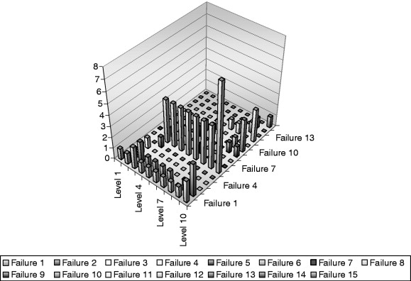
So far, we have looked only at the first occurrence of the failure. The next item to look at is the repetition of the failures. Figure 26.16, the histogram of the failures vs. the level in which the failures occurred vs. how often the failure occurred, provides several important clues. With a statistical test, outliers are identified by their deviation from the mean relative to the standard deviation of the population. During the FMVT (which is often on only one system), when a failure occurs, the item that fails is repaired or replaced. Naturally, if the failure that occurred is inherent to the design and not just an artifact of the particular fabrication, the failure will occur again and again. In the histogram of the toothbrush failures, you can see that the bristles falling out occurs over and over again. However, the rubber insert delaminating does not occur as often.

Figure 26.16. Histogram of toothbrush failures.

In some cases, the histogram will show a failure that occurs once very early and then never repeats. This type of failure is usually the results of a fabrication issue. This does not mean the failure should be ignored. In fact, the differentiation between repeatable, design-inherent failures and fabrication issues is one of the very powerful results of an FMVT. Knowing that a particular fabrication step can easily result in an early failure allows the production process to target controls on critical steps. The histogram from an FMVT is an effective tool for sorting out between design-inherent failures and fabrication issues.

In the case of the toothbrush, the failure-mode progression is failure small. A more complex failure mode progression may be the controller data shown in Figure 26.17. In this case, the design maturity calculations become very important in sorting out the failures. (See Table 26.7.)

Figure 26.17. Controller failure mode progression.

Table 26.7. Controller design maturity and predicted design maturity

	DM	Change
DM	0.767857
PDM1	0.270154	0.497703
PDM2	0.289683	−0.019529
PDM3
PDM4	0.248148	0.067869
PDM5
PDM6	0.194005	0.055038
PDM7	0.221719	−0.027715
PDM8	0.170251	0.051469
PDM9	0.158095	0.012156
PDM10	0.13843	0.019665
PDM11	0.12745	0.010979
PDM12	0.056213	0.071238

You can see here that the design maturity and the predicted design maturity is a bit more complex. You can also see that fixing the first failure reduces the potential for improvement from around 76% to 27%, but then fixing failures makes the measure worse. This is because the second three failures are clustered together. This is important in evaluating what failures to fix and which ones to leave. There is not much sense in fixing the second failure, unless you are also going to address the other two failures. This is also true for the fifth and sixth failure and the seventh and eighth failure (keep in mind that PDM5 means the first five have been addressed and you are looking at the potential of fixing the sixth). After fixing the seventh failure, the trend is continuously better.

The histogram for the controller data (Figure 26.18) shows more clearly the use of the histogram to sort failures. Notice that the first two failures are very repeatable and happen early—definite targets for improving the design. The third–fifth failures all occur once very early and then never repeat. These failures are likely fabrication errors. Knowing this changes the decisions that may be made about the second failure. From the failure mode progression and the PDM analysis, it was noted that the second–fourth failures should be addressed as a group. However, the histogram indicates that the third and fourth failures are fabrication related. They will be addressed through production controls separately from the second failure, which is a design-inherent failure mode.

Figure 26.18. Histogram of controller failures.

One other consideration can be made in examining failures from a complex system, and that is to sort the failure mode progression based on severity or subsystem. In this case, the controller failure mode progression is separated into three progressions. (See Figure 26.19.) One for mild, medium and severe failures. This can also help identify which failures are worth fixing and which are not.

Figure 26.19. Ranked failure mode progression of controller.

26.15. Comparison FMVT

FMVT measures the progression of failures and estimates which failures should be fixed and which are normal end-of-life wear out of an optimized design. By comparing the failure mode progression of an existing design and a new design, a comparison of the quality of the new design to the old design can be made on two key points: time to first failure and optimization or failure-mode progression.

Provided that known field references, such as best-in-class, best-in-world, or best-in-company designs are available, a simple FMVT comparison can be conducted in two ways.

26.16. Method 1. Time to First Failure

In this method, a design exists for which relative field performance is known (for example, a three-year warranty rate of 0.96%), an FMVT is conducted on a sample of the existing design. After the test is complete, the test level at which the first relevant failure occurred is identified. A new sample of the existing design and a sample of the new design are tested at the identified level until both fail. The time to failure of the two samples is used to scale the field performance of the existing design to provide an expected field performance of the new design.

For example,

• Existing design MTTF in the field is 67 months
• First hard failure occurred at level 7
• Existing design time to failure at level 7 is 243 minutes
• New design time to failure at level 7 is 367 minutes
• Estimated new design MTTF = (67 mon/243 min)
• 367 min = 101 mon

This method can be used with multiple reference samples to establish an expected range. In other words, instead of comparing to one existing design, compare to two or three designs. The results will vary slightly but will provide an estimated range in which the new design is expected to perform.

26.17. Method 2. Failure-Mode Progression Comparison

In this method, the existing design and the new design both go through a complete FMVT and the comparison is conducted on the full list of failure modes and their relative distribution. This is a more thorough comparison because it evaluates the time to first failure and also the efficiency of the design. An estimate on the improvement in the design for field performance can be made from the design maturity quantification of failure-mode progression.

26.18. FMVT Life Prediction—Equivalent Wear and Cycle Counting

When using a broad range of stress sources in an accelerated test plan and a broad range of failure mechanisms is present, a life prediction can be made if the damage accumulated is proportional for all of the different mechanisms.

An example of this is a test conducted on an automotive window regulator, in which metal-on-metal wear, metal fatigue, plastic-on-metal wear, and threaded fastener torque loss were the failure modes. In this particular case, the accumulated damage on these different failure mechanisms could be documented and compared to the damage accumulated during a controlled life condition test. It was determined that 8 hr in an FMVT correlated to the same damage accumulated in a 417 hr life test, which correlated to one life in the field.

Using this technique, a life test was designed that took only 8 hr and quantified the life of the product through the equivalent wear.

When a door or a closure of some type is present, processing the time domain data of the door motion can make a life prediction. The motion of the closure is analyzed to “count” equivalent cycles. In this method, a cycle from the field conditions of a product (for example, a toaster oven door) is analyzed for its characteristics in displacement, velocity, acceleration, voltage, and current. A profile of one cycle is then determined as a set of conditionals (a door “open,” acceleration going negative, then positive, displacement passing through a given point, and so forth). These conditionals are then used to count the number of times a cycle (“open” event) is caused during a random (vibration, voltage, and cycling) fatigue test. The cycles are then plotted as a histogram against their severity (number of cycles with a 4-g peak spike). In this way, Minor's rule can be applied to the equivalent number of cycles and the amount of equivalent life can be determined. This method has been used on products to get a quantified life cycling test from 200 hr down to less then 8 hr (Porter, 2002).

26.19. FMVT Warranty

FMVT can be used for troubleshooting warranty issues. To accomplish this, a standard FMVT is run on the product. The emphasis is put on identifying and applying all possible stress sources. Once the standard FMVT is conducted, two possibilities exist. Either the warranty issue was reproduced, in which case the troubleshooting can go to the next stage. Otherwise, a significant fact has been established. The warranty issue is due to a stress source that was not identified or applied. If this is the case, then the additional stress source(s) must be identified and the FMVT rerun.

Once the warranty issue has been reproduced in the full FMVT, then a narrower test of limited stresses and levels is determined that will reproduce the warranty problem in a short period of time. Usually, a test that produces the warranty failure mode on the current design in only a few hours can be produced. This test can then be used to test design solutions. Once a design solution is identified, a full FMVT should be conducted.

26.20. More on Vibration

Failure-mode verification testing requires the application of a wide range of stress sources to a product. Stress sources are sources of damage to the product. The stress sources are applied to the product to induce failure modes that are inherent to the design of the product but would not otherwise be easily detectable. Stress sources are typically vibration, temperature, voltage, pressure, chemical attack, and so forth. Of all of these stress sources, the most difficult and the most critical is vibration.

Vibration is present in the working environment of any product, from automobiles to airplanes, from desktop computers to soap dispensers. In addition to being prevalent, vibration is inherently destructive. Even low levels of vibration can cause significant damage to a product. Vibration is able to do this for three reasons:

1. Vibration is a repeated event that occurs as little as several times a second to as much as tens of thousands of times a second. Imagine a debt that with payments made at the rate of $0.01 per second (1 cent every second). At that rate, a $10,000.00 debt would be paid off in 10 million seconds or just over 115 days. Vibration works the same way, doing very little (1 cent is not much) but doing it over and over again very fast.
2. Vibration is significant because of the natural frequencies that are inherent in every product. A natural frequency is the way a part “rings” like a tuning fork or a fine crystal wine glass. When a tuning fork is struck, it rings. The sound it makes is produced by the motion of the forks. This motion is called the mode shape; the shape a part moves naturally in when stimulated. Mode shapes are extremely important for vibration damage to a product. To break a product from fatigue, the product must be strained, like bending a metal coat hanger back and forth until it breaks. The tuning fork's mode shape is the shape the product will bend the most in and bend easiest in. If vibration is applied to the product at its natural frequency, the bending that results in the product will be significantly higher than if the vibration was applied at some other frequency. This relationship is expressed in the following graph in Figure 26.20. Notice that in this example, applying vibration below the natural frequency (98 Hz) has a significant effect on the level of strain damage. Applying vibration above the natural frequency results in very little strain damage. Applying vibration directly at the natural frequency causes a much larger rate of strain damage (Bastien, 2000; Henderson, 2000, 2002; Holman, 1994; Tustin, 2002). The importance of the vibration spectrum can be summed up this way: Vibration that is at or just below the natural frequency of the product being tested will provide significant contributions to the accumulated strain damage in the product.

   Figure 26.20. Potential strain damage as a function of vibration.

   

3. Vibration is critical because it contributes to the accumulation of damage from other stress sources. Vibration exacerbates thermal stresses, bearing surface wear, connector corrosion, electrical arcing, and so forth.

Vibration is critical to properly stressing a product, but vibration is made up of several components: amplitude, spectrum, and crest factor to name a few. As seen previously, the frequency at which the vibration is present is important to how effective it is in producing damage in a product. In reality, vibration exists at multiple frequencies simultaneously, not at one frequency. These multiple simultaneous frequencies are called the vibration spectrum. In this sense, mechanical vibration is much like light. Shine light through a prism and the different colors (frequencies) of light can be seen. The original light source has all of the frequencies present simultaneously. Vibration spectrums vary as widely as the colors of lights. Choosing the right spectrum requires understanding the natural frequencies of the products being tested (so that most of the spectrum is at or below the natural frequencies of the part) and knowing the spectrums that the vibration equipment can produce.

All vibration equipment has a spectrum from zero to infinity. An office table has a vibration spectrum from zero to infinity. The question is how much amplitude exists at the different frequencies. There are three physical limits that govern the amplitude on all vibration equipment: displacement, velocity, and acceleration. See Figures 26.8 through 26.10.

26.20.1. Displacement

At low-frequencies, the displacement is the limiting factor on acceleration amplitude. The laws of physics dictate that a given frequency and acceleration requires a certain displacement. At 1 Hz (1 cycle per second), a 4-g acceleration (acceleration four times greater then earth's gravity) would require nearly 1 m (just over 1 yd) of displacement. Most vibration equipment claims a spectrum down to 5 Hz. At 5 Hz, a 4-g acceleration requires 6.2 cm (2.44 in.) of displacement. Evaluating the low-requency capabilities of a machine is then easy. What is its maximum possible displacement?

26.20.2. Velocity

Velocity is a limit for some machines in the mid-frequency range. Servo-hydraulic machines are limited in the maximum velocity of the pistons used to drive the machines because of the maximum flow rate of the hydraulic supply.

26.20.3. Acceleration

Acceleration is a limit on all machines based on two factors: the mass that is being moved, and how strong the components of the machine are. Force is equal to mass times acceleration. The maximum force the machine can produce (directly or kinetically) will limit the maximum acceleration. The other consideration is that the machine must be able to withstand the forces necessary to move the mass. Maximum accelerations are usually advertised for a machine.

The amplitude at higher frequencies is also governed by damping and control methods. With most servo-hydraulic multiaxis vibration tables, the limiting factor is the natural frequency of the vibration equipment. Operating at the natural frequency of the vibration equipment would be very damaging to the capital investment. For this reason, most multiaxis servo-hydraulic equipment is limited to 70 Hz, while some have limits up to 350 Hz. Air hammer tables use the natural frequencies of the table itself to reach very high natural frequencies; the repeatability and uniformity of the tables are subject to the natural frequencies of the particular table. The upper-end of the spectrum on the FMVT machine is limited by hysteresis in the vibration mechanism dampening out the spectrum produced by the mechanical recursive equations used to produce the vibration.

26.21. Reliability and Design Maturity

Design maturity as a measure was first developed to address the issue of objectively sorting failure modes, especially in a contract situation between companies. However, the historical measure for contracts has been the statistical reliability measure. Design maturity and statistical reliability are related. (See Figure 26.21.) The bottom line is this: Statistical reliability and design maturity measure two orthogonal characteristics of the same whole. (See Figure 26.22.)

Figure 26.21. The relationship between reliability and design maturity.

Figure 26.22. Reliability and design maturity exist on orthogonal axis.

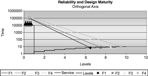
In other words, the individual failures that would be seen as a failure mode progression (along the x-axis) relate to the failures that should not be seen in a fully censored test through their respective accelerated reliability curves. With FMVT, the conscious decision is made to find the failure modes and rank them relative to each other and their stress levels and to not know the time to failure in the field or their acceleration curves.

The confidence in the failure mode progression comes from knowing that each individual failure does have an acceleration curve (stress vs. time to failure) and that curve limits how early the failure can occur in the FMVT and still meet the service time requirements. A failure that occurs at level 2 would require an impossibly steep curve to meet life requirements under service conditions.

26.22. Business Considerations

FMVT provides meaningful data (information) for the design engineer, especially during the development stages of a product. The comparison testing, equivalent wear, and cycle counting provide a means for the tool to be used for reliability estimating. For warranty chases, FMVT has proven to be a very useful tool. The design maturity analysis and the graphical tools help provide a means of relating the data to context and decisions that must be made.

The entrepreneurial business (innovative part instead of commodity) will find this tool to be especially helpful when the technology used to fabricate it is new, and understanding of how to test is limited. The brainstorming session combined with an abbreviated DFMEA has jump-started the level of understanding on many new technology validation programs.

Commodity businesses have found great use in the comparison application of FMVT to conduct design of experiments extremely quickly on complex, multistress environment products. This has worked well in team-based corporate structures.

FMVT does introduce a significant problem for the top-down management structure. Namely, the results of the test are highly technical, require engineering thought and evaluation and are not a clear pass/fail result that is simple for the 10,000 ft view VP to grasp in 15 s. A top-down business structure will require significant education of the middle and upper management on how to interpret the results, what kind of questions to ask, and how to make decisions from a DM, TL, and failure-mode progression. It is not rocket science, but it has not been around for 100+ years like statistics has.

Key facts going forward:

1. If you miss a stress source, you will miss a failure
2. If you are not going to spend some time understanding the results, do not do the test