
Chapter 18 Heat, beat, stick and polish: Manufacturing processes
- 18.1 Introduction and synopsis 422
- 18.2 Process selection in design 422
- 18.3 Process attributes: material compatibility 424
- 18.4 Shaping processes: attributes and origins 426
- 18.5 Joining processes: attributes and origins 434
- 18.6 Surface treatment (finishing) processes: attributes and origins 437
- 18.7 Estimating cost for shaping processes 438
- 18.8 Computer-aided process selection 442
- 18.9 Case studies 443
- 18.10 Summary and conclusions 453
- 18.11 Further reading 454
- 18.12 Exercises 454
- 18.13 Exploring design with CES 455
- 18.14 Exploring the science with CES Elements 457
Materials and processing are inseparable. Ores, minerals and oil are processed to create the stuff of engineering in clean, usable form. These are shaped into components, finished and joined to make products. Chapter 2 defined a hierarchy for these processes; in this chapter we explore their technical capabilities and methods for choosing which to use. Increasingly, legislation and public opinion require that materials are recycled at the end of product life. New processes are emerging to extract usable material from what used to be regarded as waste.
18.1 Introduction and synopsis
Materials and processing are inseparable. Ores, minerals and oil are processed to create the stuff of engineering in clean, usable form. These are shaped into components, finished and joined to make products. Chapter 2 defined a hierarchy for these processes; in this chapter we explore their technical capabilities and methods for choosing which to use. Increasingly, legislation and public opinion require that materials are recycled at the end of product life. New processes are emerging to extract usable material from what used to be regarded as waste.
The strategy for choosing a process parallels that for materials: screen out those that cannot do the job, rank those that can (usually seeking those with the lowest cost) and explore the documented knowledge of the top-ranked candidates. Many technical characteristics of a process can be described by numeric and nonnumeric data: the size of part it can produce, the surface finish of which it is capable and, critically, the material families or classes it can handle and the shapes it can make. Constraints on these provide the inputs for screening, giving a short list of processes that meet the requirements of the design.
There is another aspect to this. It relates to the influence of processing on the properties of the materials themselves. Materials, of course, have properties before they are shaped, joined or finished, and processing is used to enhance properties such as strength. But the act of processing can also damage properties by introducing porosity, cracks and defects or by changing the microstructure in a detrimental way. These interactions, central to the choice and control of processes, are explored further in Chapter 19. For now, it is sufficient to recognise that success in manufacturing often relies on accumulated know-how and expertise, resident, in the past, in the heads of long-established employees but now captured as design guidelines, best practice guides and software providing the information needed for the documentation stage.
18.2 Process selection in design
The selection strategy
The taxonomy of manufacturing processes was presented in Chapter 2. There, it was established that processes fall into three broad families: shaping, joining and finishing (Figures 2.4 and 2.5). Each is characterised by a set of attributes listed, in part, in Figures 2.6 and 2.7.
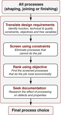
The strategy for materials selection was outlined in Chapter 3. The procedure, whether dealing with original design or refining an existing one, was to translate the design requirements into a set of constraints and objectives. The constraints are used to screen and the objectives to rank, delivering a preferred short-list of materials that best meet both, finally seeking documentation to guide the final choice. The strategy for selecting processes follows a parallel path, shown in Figure 18.1. It uses constraints on process attributes to screen, together with an appropriate objective to rank, culminating as before with a search for information documenting the details of the top-ranked candidates.
Translation
As we saw in earlier chapters, the function of a component dictates the initial choice of material and shape. This choice exerts constraints on the choice of processes. It is helpful to think of two types of constraint: technical—can the process do the job at all? And quality—can it do so sufficiently well? One technical constraint applies across all process families: it is the compatibility of material and process. Shape, too, is a general constraint, although its influence on the choice of shaping, joining and finishing processes differs. Quality includes precision and surface finish, together with avoidance of defects and achieving the target for material properties. The usual objective in processing is to minimise cost. The free variables are largely limited to choosing the process itself and its operating parameters (such as temperatures, flow rates and so on). Table 18.1 summarises the outcome of the translation stage. The case studies of Section 18.9 illustrate its use for each process family.
Table 18.1 Function, constraints, objective and free variables
| Function | •What does the process do? |
| Constraints | •What technical and quality limits must be met? |
| Objective | •Minimise cost |
| Free variables | •Choice of process and process operating conditions |
Screening
Translation, as with materials, leads to constraints for process attributes. The screening step applies these, eliminating processes that cannot meet the constraints. Some process attributes are simple numeric ranges—the size or mass of component the process can handle, the precision or the surface smoothness it can achieve. Others are non-numeric—lists of materials to which the process can be applied, for example. Requirements such as ‘made of magnesium and weighing about 3 kg’ are easily compared with the process attributes to eliminate those that cannot shape magnesium or cannot handle a component as large (or as small) as 3 kg.
Ranking
Ranking, it will be remembered, is based on objectives. The most obvious objective in selecting a process is that of minimising cost. In certain demanding applications it may be replaced by the objective of maximising quality regardless of cost, though more usually it is a trade-off between the two that is sought.
Documentation
Screening and ranking do not cope adequately with the less tractable issues (such as corrosion behaviour); they are best explored through a documentation search. This is just as true for processes. Old hands who have managed a process for decades carry this information in their heads and can develop an almost mystical ability to detect problems that defy immediate scientific explanation. But jobs for life are rare today; experts move, taking their heads with them. Expertise is stored more accessibly in compilations of design guidelines, best practice guides, case studies and failure analyses. The most important technical expertise relates to productivity and quality. Machines all have optimum ranges of operating conditions under which they work best and produce products with uncompromised quality. Failure to operate within this window can lead to manufacturing defects, such as excessive porosity, cracking or residual stress. This in turn leads to scrap and lost productivity, and, if passed on to the user, may cause premature failure. At the same time material properties depend, to a greater or lesser extent, on process history through its influence on microstructure. Processes are chosen not just to make shapes but to fine-tune properties.
So, documentation and knowledge of how processes work (or don’t work) are critical in design. There is only so far that screening and ranking can take us in finding the right process.
18.3 Process attributes: material compatibility
The main goal in defining process attributes is to identify the characteristics that discriminate between processes, to enable their selection by screening. Each of the three process families—shaping, joining and surface treatment—has its own set of characterising attributes, described here and in the next three sections. It is also of interest to explore the physical limits to these for a given process, and to examine how the properties of the material being processed limit the rate of the process itself.
One process attribute applies to all three families—compatibility with material—so we examine this first.
Material–process compatibility
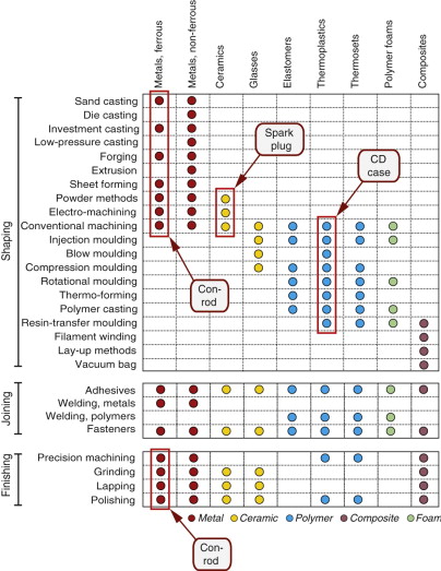
Figure 18.2 shows a material–process compatibility matrix. Shaping processes are at the top, with compatible combinations marked by dots the colour of which identifies the material family. Its use for screening is straightforward—specify the material and some processes are immediately eliminated (or the reverse, as a screening step in material selection). The diagonal spread of the dots in the matrix reveals that each material class—metals, polymers, etc.—has its own set of process routes. This largely reflects the underlying process physics. Shaping is usually eased by melting or softening the material, and the melting temperatures of the material classes are quite distinct (Figure 13.6). There are some overlaps—powder methods are compatible with both metals and ceramics, moulding with both polymers and glasses. Machining (when used for shaping) is compatible with almost all families. Joining processes using adhesives and fasteners are very versatile and can be used with most materials, whereas welding methods are material specific. Finishing processes are used primarily for the harder materials, particularly metals—polymers are moulded to shape and rarely treated further except for decorative purposes. We will see why later.
Coupling of material selection and process selection
The choices of material and of process are clearly linked. The compatibility matrix shows that the choice of material isolates a subdomain of processes. The process choice feeds back to material selection. If, say, aluminum alloys were chosen in the initial material selection stage and casting in the initial process selection stage, then only the subset of aluminum alloys that are castable can be used. If the component is then to be age hardened (a heat-treatment process), material choice is further limited to heat-treatable aluminum casting alloys. So we must continually iterate between process and material, checking that inconsistent combinations are avoided. The key point is that neither material nor process choice can be carried too far without giving thought to the other. Once past initial screening, it is essentially a coselection procedure.
18.4 Shaping processes: attributes and origins
Mass and section thickness
There are limits to the size of component that a process can make. Figure 18.3 shows the limits. The colour coding for material compatibility has been retained, using more than one colour when the process can treat more than one material family. Size can be measured by volume or by mass, but since the range of either one covers many orders of magnitude, whereas densities span only a factor of about 10, it doesn’t make much difference which we use—big things are heavy, whatever they are made of. Most processes span a mass range of about a factor of 1000 or so. Note that this attribute is most discriminating at the extremes; the vast majority of components are in the 0.1 to 10 kg range, for which virtually any process will work.
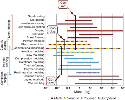
Figure 18.3 The process–mass range bar chart for shaping processes. Ignore, on first reading, the boxes; they refer to case studies to come. The colours refer to the material, as in Figure 18.2. Multiple colours indicate compatibility with more than one family.
It is worth noting what the ranges represent. Each bar spans the size range of which the process is capable without undue technical difficulty. All can be stretched to smaller or larger extremes but at the penalty of extra cost because the equipment is no longer standard. During screening, therefore, it is important to recognise ‘near misses’—processes that narrowly failed, but that could, if needed, be reconsidered and used.
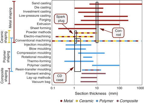
Figure 18.4 shows a second bar chart: that for the ranges of section thickness of which each shaping process is capable. It is the lower end of the ranges—the minimum section thickness—where the physics of the process imposes limits. Their origins are the subject of the next subsection.
Physical limits to size and section thickness
Casting and moulding both rely on material flow in the liquid or semi-liquid state. Lower limits on section thickness are imposed by the physics of flow. Viscosity and surface tension oppose flow through narrow channels, and heat loss from the large surface area of thin sections cools the flowing material, raising the viscosity before the channel is filled (Figure 18.5). Polymer and glass viscosities increase steadily as temperature drops. Pure metals solidify at a fixed temperature, with a step increase in viscosity, but for alloys this happens over a range of temperature, known as the ‘mushy zone’, in which the alloy is part liquid, part solid. The width of this zone can vary from a few degrees centigrade to several hundred—so metal flow in castings depends on alloy composition. In general, higher pressure die-casting and moulding methods enable thinner sections to be made, but the equipment costs more and the faster, more turbulent flow can entrap more porosity and cause damage to the moulds.
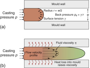
Figure 18.5 Flow of liquid metal or polymer into thin sections is opposed by surface tension (a) and by viscous forces (b). Loss of heat into the mould increases viscosity and may cause premature solidification.
Upper limits to size and section in casting and moulding are set by problems of shrinkage. The outer layer of a casting or moulding cools and solidifies first, giving it a rigid skin. When the interior subsequently solidifies, the change in volume can distort the product or crack the skin, or cause internal cavitation. Problems of this sort are most severe where there are changes of section, since the constraint introduces tensile stresses that cause hot tearing—cracking caused by constrained thermal contraction. Different compositions have different susceptibilities to hot tearing—another example of coupling between material, process and design detail.
Much of the documentation for casting and moulding processes concerns guidance on designing both the component shape and the mould geometry to achieve the desired cross-sections while avoiding defects. Even when the component shape is fixed, there is freedom to choose where the material inlets are built into the mould (the ‘runners’) and where the air and excess material will escape (the ‘risers’). Figure 18.6 shows an example of good practice in designing the cross-sectional shape of a polymer moulding.
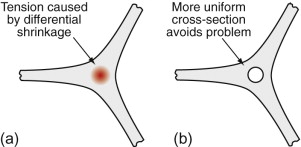
Figure 18.6 (a) Differential shrinkage causes internal stress, distortion and cavitation in thick sections or at changes of section. (b) Good design keeps section thickness as uniform as possible, avoiding the problem.
Powder methods for metals and ceramics, too, depend on flow. Filling a mould with powder uses free flow under gravity plus vibration to bed the powder down and achieve uniform filling. This may be followed by compression (‘cold compaction’). Once full of powder, the mould is heated to allow densification by sintering or, if the pressure is maintained, by hot isostatic pressing (HIPing).
Metal shaping by deformation—hot or cold rolling, forging or extrusion—also involves flow. Solid metals flow by plastic deformation or by creep—Chapter 13 described how the flow rate depends on stress and temperature. Much forming is done hot because the hot yield stress is lower than that at room temperature and work hardening, which drives the yield strength up during cold deformation, is absent. The thinness that can be rolled, forged or extruded is limited by plastic flow in much the same way that the thinness in casting is limited by viscosity: the thinner the section, the greater the required roll-pressure or forging force.
Figure 18.7 illustrates the problems involved in forging or rolling very thin sections. Friction changes the pressure distribution on the die and under the rolls. When they are well lubricated, as in (a), the loading is almost uni-axial and the material flows at its yield stress σy. With friction, as in (b), the metal shears at the die interface and the pressure ramps up because the friction resists the lateral spreading, giving a ‘friction hill’. The area under the pressure distribution is the total forming load, so friction increases the load. The greater the aspect ratio of the section (width/thickness), the higher the maximum pressure needed to cause yielding, as in (c). This illustrates the fundamental limit of friction on section thickness—very thin sections simply stick to the tools and will not yield, even with very large pressures. Friction not only increases the load and limits the aspect ratio that can be formed, it also produces distortion in shape—‘barrelling’—shown in both (b) and (c). A positive aspect of the high contact pressures in forging is the repeatability with which the metal can be forced to take up small features machined on the face of the tooling, exploited in making coins.
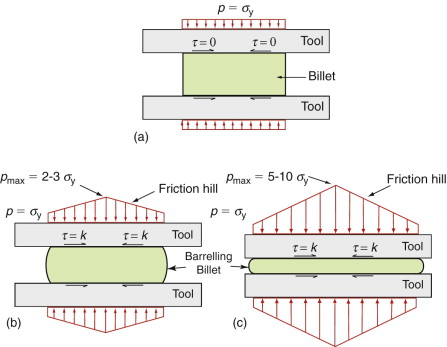
Figure 18.7 The influence of friction and aspect ratio on open die forging. (a) Uniaxial compression with very low friction. (b) With sticking friction the contact pressure rises in a ‘friction hill’ causing barrelling. (c) The greater the aspect ratio, the greater the pressure rise and the barrelling.
Very small or very thin objects—pushing the limits
So how do you make very small things? The obvious way to do it is to cut them out of bigger ones. That means machining: turning, shaping, drilling and milling. The upper limit on size is set by the budget available to buy the machine and the electricity bill for its use. Lower limits—now we are thinking of milligrams and fractions of a millimeter—are set by the stiffness of the machine and the material itself.
One continuous shaping process, rolling, is able to produce sections as thin as 10 µm—the thickness of aluminum kitchen foil. The foil only yields and thins just as it enters and leaves the roll bite—in between, the huge aspect ratio and frictional constraint mean that the high pressure actually flattens the steel rolls elastically. The process is helped by ‘pack rolling’—feeding two sheets through together, with lubricant in between so that they can be peeled apart as they exit the rolls. This is why kitchen foil is shiny on one side (where contact was with the roll) and matt on the other.
Suppose you want to go still smaller. Flow won’t work, and the sections are so thin that they simply bend if you try to machine them. Now you need chemistry. Conventional chemistry—etching, chemical milling, electro-discharge milling—allows features on the same scale as that of precision machining. To get really small, we need the screening, printing and etching techniques used to fabricate electronic devices. These are used to make MEMS (micro-electro-mechanical systems)—tiny sensors, actuators, gears and even engines. At present the range of materials is limited by this silicon-based technology, but some commercial devices, such as the inertial triggers for airbags, are made in this way.
Shape
A key attribute of a process is the families of shapes it can make. It is also one of the most difficult to characterise. A classification scheme is illustrated in Figure 18.8, with three generic classes of shape, each subdivided in two. The merit of this approach is that processes map onto specific shapes. Figure 18.9 shows the matrix of viable combinations.
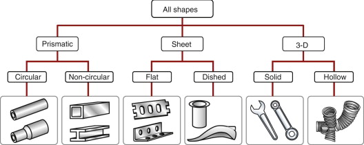
Figure 18.8 The classification of shape. Subdivision into more than six classes is difficult, and does not give useful further discrimination.
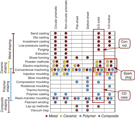
Figure 18.9 The shape–process compatibility matrix. A dot indicates that the pair forms a viable combination colour-coded as before.
The prismatic shapes shown on the left of Figure 18.8, made by rolling, extrusion or drawing, have a special feature: they can be made in continuous lengths. The other shapes cannot—they are discrete, and the processes that make them are called batch processes. The distinction between continuous and discrete (or batch) processes is a useful one, bearing on the cost of manufacture. Batch processes require repeated cycles of setting-up, which can be time-consuming and costly. On the other hand, they are often net-shape or nearly so, meaning that little further machining is needed to finish the component. Casting and moulding processes are near net-shape. Forging, on the other hand, is limited by the strains and shape changes by solid-state plasticity, starting from standard stock (bar, rod or sheet) to create a 3-D shape in several stages requiring a sequence of dies.
Continuous processes are well suited to long, prismatic products such as railway track or standard stock material such as tubes, plate and sheet. Cylindrical rolls produce sheets. Shaped rolls make more complex profiles—rail track is one of these. Extrusion is a particularly versatile continuous process, since complex prismatic profiles that include internal channels and longitudinal features such as ribs and stiffeners can be manufactured in one step.
Tolerance and roughness
We think of the precision and surface finish of a component as aspects of its quality. They are measured by the tolerance, T, and the surface roughness, R. When the dimensions of a component are specified the surface quality is specified as well, though not necessarily over the entire surface. Surface quality is critical in contacting surfaces such as the faces of flanges that must mate to form a seal or sliders running in grooves. It is also important for resistance to fatigue crack initiation and for aesthetic reasons. The tolerance T on a dimension y is specified as y = 100 ± 0.1 mm, or as y = ![]() mm, indicating that there is more freedom to oversize than to undersize. Surface roughness, R, is specified as an upper limit, for example, R < 100 µm. The typical surface finish required in various products is shown in Table 18.2. The table also indicates typical processes that can achieve these levels of finish.
mm, indicating that there is more freedom to oversize than to undersize. Surface roughness, R, is specified as an upper limit, for example, R < 100 µm. The typical surface finish required in various products is shown in Table 18.2. The table also indicates typical processes that can achieve these levels of finish.
Table 18.2 Typical levels of finish required in different applications, and suitable processes
| Roughness (µm) | Typical application | Process |
|---|---|---|
| R = 0.01 | Mirrors | Lapping |
| R = 0.1 | High-quality bearings | Precision grind or lap |
| R = 0.2–0.5 | Cylinders, pistons, cams, bearings | Precision grinding |
| R = 0.5–2 | Gears, ordinary machine parts | Precision machining |
| R = 2–10 | Light-loaded bearings, noncritical | Machining components |
| R = 3–100 | Nonbearing surfaces | Unfinished castings |
Surface roughness is a measure of the irregularities of the surface (Figure 18.10). It is defined as the root-mean-square (RMS) amplitude of the surface profile:
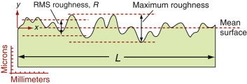
Figure 18.10 A section through a surface, showing its irregular surface (artistically exaggerated in the vertical direction). The irregularity is measured by the RMS roughness, R.
It used to be measured by dragging a light, sharp stylus over the surface in the x-direction while recording the vertical profile y(x), like playing a gramophone record. Optical profilometry, which is faster and more accurate, has now replaced the stylus method. It scans a laser over the surface using interferometry to map surface irregularity. The tolerance T is obviously greater than 2R; indeed, since R is the root-mean-square roughness, the peak roughness, and hence absolute lower limit for tolerance, is more like 5R. Real processes give tolerances that range from 10R to 1000R.
Figures 18.11 and 18.12 show the characteristic ranges of tolerance and roughness of which processes are capable, retaining the colour coding for material family. Data for finishing processes are added below the shaping processes. Sand casting gives rough surfaces; casting into metal dies gives a smoother one. No shaping processes for metals, however, do better than T = 0.1 mm and R = 0.5 µm. Machining, capable of high dimensional accuracy and surface finish, is used commonly after casting or deformation processing to bring the tolerance or finish up to the desired level, creating a process chain. Metals and ceramics can be surface-ground and lapped to a high precision and smoothness: a large telescope reflector has a tolerance approaching 5 µm and a roughness of about 1/100 of this over a dimension of a metre or more. But precision and finish carry a cost: processing costs increase exponentially as the requirements for both are made more severe. It is an expensive mistake to overspecify precision and finish.
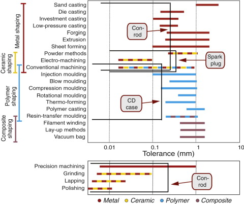
Figure 18.11 The process–tolerance bar chart for shaping processes and some finishing processes, enabling process chains to be selected. The chart is colour-coded by material and annotated with the target values for the case studies.
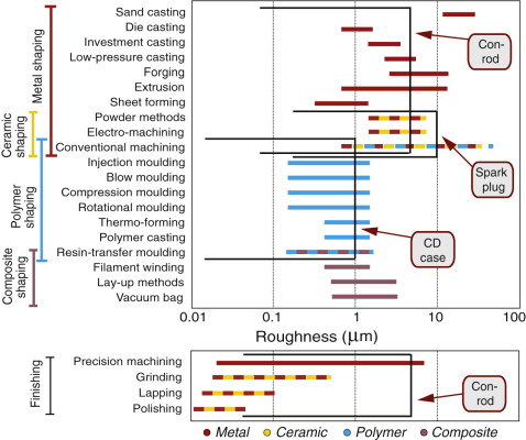
Figure 18.12 The process–roughness bar chart for shaping processes and some finishing processes, enabling process chains to be selected.
Moulded polymers inherit the finish of the moulds and thus can be very smooth (Figure 18.12); machining to improve the finish is rarely necessary. Tolerances better than ±0.2 mm are seldom possible (Figure 18.11) because internal stresses left by moulding cause distortion and because polymers creep in service.
18.5 Joining processes: attributes and origins
The design requirements to be met in choosing a joining process differ from those for choosing a shaping process. Even material compatibility is more involved than for shaping, in that joints are often to be made between dissimilar materials.
Material compatibility
Processes for joining metals, polymers, ceramics and glasses differ. Adhesives will bond to some materials but not to others; methods for welding polymers differ from those for welding metals; and specific metals often require specific types of welds. The material-process matrix (Figure 18.2) includes four classes of joining process.
When the joint is between dissimilar materials, further considerations arise, both in manufacture and in service. The process must obviously be compatible with both materials. Adhesives and fasteners generally allow joints between different materials; many welding processes do not. Practicality in service is a different issue. If two materials are joined in such a way that they are in electrical contact, a corrosion couple appears if close to water or a conducting solution. This can be avoided by inserting an insulating interlayer between the surfaces. Thermal expansion mismatch gives internal stresses in the joint if the temperature changes, with risk of damage. Identifying good practice in joining dissimilar materials is part of the documentation step.
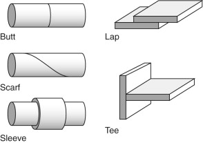
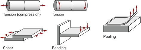
Joint geometry and mode of loading
Important joining-specific considerations are the geometry of the joint, the thickness of material they can handle and the way the joint will be loaded. Figures 18.13 and 18.14 illustrate standard joint geometries and modes of loading. The choice of geometry depends on the shapes and thicknesses of the parts to be joined, and the mode of loading—it is a coupled problem. Adhesive joints support shear but are poor in peeling—think of peeling off sticky tape. Adhesives need a good working area—lap joints are fine, butt joints are not. Rivets and staples, too, are well adapted for shear loading of lap joints but are less good in tension. Welds and threaded fasteners are more adaptable, but here, too, matching choice of process to geometry and loading is important. Screening on each in isolation correctly keeps options open, but the details of the coupling must be researched at the documentation stage.
When making joints, sheet thickness is an issue. Joining processes like stapling, riveting and sewing can be used with thin sections but not with thick. The thickness that can be welded is restricted, to varying degrees, by heat transfer considerations. Some processes are better adapted than others to joining greatly unequal sections: adhesives can bond a very thin layer to a very thick one, whereas riveting and sewing work best for sections that are nearly equal. In practice the thickness, too, is coupled to geometry.
Secondary functionalities and manufacturing constraints
Most joints carry load, but that is not all. Joints may need to conduct or insulate against the conduction of heat or electricity, or they may be required to operate at an elevated operating temperature. A joint may also serve as a seal, and be required to exclude gases or liquids.
Manufacturing conditions also impose constraints on joint design. Certain joining processes impose limits on the size of the assembly; electron beam welding, for instance, usually requires that the assembly fit within a vacuum chamber. On-site joining operations conducted out of doors require portable equipment, possibly with portable power supplies; an example is the hot-plate welding of PVC and PE pipelines. Portability, on the other hand, effectively means there is no limit on the size of the assembly—bridges, shipbuilding and aircraft make this self-evident.
An increasingly important consideration is the requirement for economic disassembly at the end of product life to facilitate recycling and reuse. Threaded fasteners can be disassembled and adhesives can be loosened with solvents or heat.
Physical limits in joining
Thermal joining processes—arc, laser and friction welding, for example—operate by imposing a local thermal cycle to the joint area to produce a bond in the liquid or solid state. Heat transfer and conduction set the physical limit to the size of joint. Here the intensity of heating is important. For translating heat sources of power Q moving at speed v along the joint line, the heat input per unit length, Q/v (J/m), commonly is used as a characteristic welding parameter. Peak temperatures and cooling rates with Q/v. Heat input is thus important in determining the extent of the ‘heat-affected zone’—the region round the weld affected by the thermal cycle imposed. The microstructural changes induced depend on the peak temperature and the cooling rate—especially in steels, which are commonly joined by welding. And local thermal cycles induce internal residual stresses. Because of their importance, microstructural changes during welding have been researched in depth and are now well understood; handbooks on the subject provide extensive documentation.
Process economics are dictated by the set-up time and the actual time for making the joint. For thermal processes, conduction of heat governs the operating speed with a given level of power, both in making the joint and in cooling of the component before it can be handled and moved. Some adhesives require prolonged curing times before they can take load, again slowing the throughput. And many processes take much longer to set up than to make the joint itself, you need to avoid misalignment or lack of cleanliness in the joint region. Inventive workstation design can help to improve the economics by arranging that multiple set-up and product cooling areas run in parallel with a high-speed joining machine, a strategy used to enable the economic performance of capital-intensive processes like laser and electron beam welding.
18.6 Surface treatment (finishing) processes: attributes and origins
Material compatibility
Material–process compatibility for surface treatments is shown at the bottom of the matrix in Figure 18.2. As noted previously, surface finishing is more important for metals than for polymers.
The purpose of the treatment
The most discriminating finishing-specific attribute proves to be the purpose of applying the treatment. Table 18.3 illustrates the diversity of functions that surface treatments can provide. Some protect, some enhance performance, still others are primarily aesthetic. All surface treatments add cost but the added value can be large. Protecting a component surface extends product life and increases the interval between maintenance cycles. Coatings on cutting tools enable faster cutting speeds and greater productivity. And surface hardening processes may enable the substrate alloy to be replaced with a cheaper material—for example, using a plain carbon steel with a hard carburised surface or a coating of hard titanium nitride (TiN), instead of using a more expensive alloy steel.
Table 18.3 The design functions provided by surface treatments
Secondary compatibilities
Material compatibility and design function are the first considerations in selecting a finishing process. But there are others. Some surface treatments leave the dimensions, precision and roughness of the surface unchanged. Deposited coatings obviously change the dimensions a little, but may still leave a perfectly smooth surface. Others build up a relatively thick layer with a rough surface, requiring refinishing. Component geometry also influences the choice. ‘Line-of-sight’ deposition processes coat only the surface at which they are directed, leaving inaccessible areas uncoated; others, with what is called ‘throwing power’, coat flat, curved and re-entrant surfaces equally well. Many surface-treatment processes require heat. These can only be used on materials that can tolerate the rise in temperature. Some paints are applied cold, but many require a bake at up to 150 °C. Heat treatments like carburising or nitriding to give a hard surface layer require prolonged heating at temperatures up to 800 °C. This thermal exposure of the substrate can change the underlying microstructure, not necessarily for the better. There are some innovative developments to match the thermal treatments required in both substrate and surface, achieving two treatments in one go. An example is the paint-bake cycle for heat-treatable aluminum alloy automotive panels, which cures and hardens the paint while simultaneously age hardening the sheet itself.
Physical limits to surface treatments
For thermal processes, the surface heating intensity and absorptivity, and the thermal properties of the substrate, dictate the rise time in temperature. For a stationary heat source of given power density, the temperature rises with the square root of time ![]() . This in turn determines the depth of surface layer that reaches the temperature at which the desired microstructural change takes place. Since diffusion of matter and heat follows the same mathematical equations, the depth of treatment in diffusion processes such as carburising has the same dependence on time. For a spray-coating process delivering a given volumetric flow rate, the coating thickness increases linearly with time.
. This in turn determines the depth of surface layer that reaches the temperature at which the desired microstructural change takes place. Since diffusion of matter and heat follows the same mathematical equations, the depth of treatment in diffusion processes such as carburising has the same dependence on time. For a spray-coating process delivering a given volumetric flow rate, the coating thickness increases linearly with time.
18.7 Estimating cost for shaping processes
Estimating process costs accurately—at the precision needed for competitive contract bidding, for example—is a specialised job. It is commonly based on interpolation or extrapolation of known costs for similar, previous jobs, appropriately scaled. Our interest here is not in estimating cost for this purpose; it is to compare approximate costs of alternative process routes. This can be useful even when imprecise. We illustrate the method with a cost model for one of the most common choices: that of a batch shaping process. It requires certain user-specified inputs, such as local labor costs, as well as values for cost-related attributes of each process.
The cost model
The manufacture of a component consumes resources (Figure 18.15), each of which has an associated cost. The final cost is the sum of those of the resources it consumes. They are defined in Table 18.4. Thus, the cost of producing a component of mass m entails the cost Cm ($/kg) of the materials and consumable feed-stocks from which it is made. It involves the cost of dedicated tooling, Ct ($), and that of the capital equipment, Cc ($), in which the tooling will be used. It requires time, chargeable at an overhead rate ![]() (thus with units of $/h), in which we include the cost of labor, administration and general plant costs. It requires energy, which is sometimes charged against a process step if it is very energy intensive, but more usually is treated as part of the overhead and lumped into
(thus with units of $/h), in which we include the cost of labor, administration and general plant costs. It requires energy, which is sometimes charged against a process step if it is very energy intensive, but more usually is treated as part of the overhead and lumped into ![]() , as we shall do here. Finally, there is the cost of information, meaning that of research and development, royalty or license fees; this, too, we view as a cost per unit time and lump it into the overhead.
, as we shall do here. Finally, there is the cost of information, meaning that of research and development, royalty or license fees; this, too, we view as a cost per unit time and lump it into the overhead.
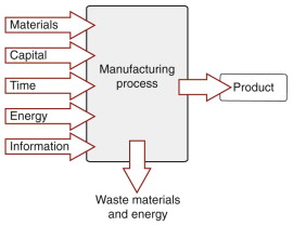
Table 18.4 Symbols, definitions and units in the cost model
| Resource | Symbol | Unit | |
|---|---|---|---|
| Materials: | Including consumables | Cm | $/kg |
| Capital: | Cost of tooling | Ct | $ |
| Cost of equipment | Cc | $ | |
| Time: | Overhead rate, including labor, administration, rent, etc. |
|
$/h |
| Energy: | Cost of energy | Ce | $/h |
| Information: | R & D or royalty payments | Ci | $/year |
Consider now the manufacture of a component (the ‘unit of output’) weighing m kg, and made of a material costing Cm $/kg. The first contribution to the unit cost is that of the material mCm. Processes rarely use exactly the right amount of material but generate a scrap fraction f, which ends up in runners, risers, machining swarf and rejects. Some is recycled, but the material cost per unit needs to be magnified by the factor 1/(1 − f) to account for the fraction that is lost. Hence the material contribution per unit is:
The cost Ct of a set of tooling—dies, moulds, fixtures and jigs—is what is called a dedicated cost: one that must be wholly assigned to the production run of this single component. It is written off against the numerical size n of the production run. However, tooling wears out at a rate that depends on the number of items processed. We define the tool life nt as the number of units that a set of tooling can make before it has to be replaced. We have to use one tooling set even if the production run is only one unit. But each time the tooling is replaced there is a step up in the total cost to be spread over the whole batch. To capture this with a smooth function, we multiply the cost of a tooling set Ct by (1 + n/nt). Thus, the tooling cost per unit takes the form:
The capital cost of equipment, Cc, by contrast, is rarely dedicated. A given piece of equipment—a powder press, for example—can be used to make many different components by installing different die-sets or tooling. It is usual to convert the capital cost of nondedicated equipment and the cost of borrowing the capital itself into an overhead by dividing it by a capital write-off time, two, (5 years, say) over which it is to be recovered. The quantity Cc/two is then a cost per hour—provided the equipment is used continuously. That is rarely the case, so the term is modified by dividing it by a load factor, L—the fraction of time for which the equipment is productive. This gives an effective hourly cost of the equipment, like a rental charge, even though it is your own piece of kit. The capital contribution to the cost per unit is then this hourly cost divided by the production rate/hour ![]() at which units are produced:
at which units are produced:
Finally, there is the general background hourly overhead rate ![]() for labor, energy and so on. This is again converted to a cost per unit by dividing by the production rate
for labor, energy and so on. This is again converted to a cost per unit by dividing by the production rate ![]() units per hour:
units per hour:

The total shaping cost per part, Cs, is the sum of these four terms, C1−C4, taking the form:
To emphasise the simple form of this equation, it can be written:
This equation shows that the cost has three essential contributions—a material cost per unit of production that is independent of batch size and rate, a dedicated cost per unit of production that varies as the reciprocal of the production volume (1/n), and a gross overhead per unit of production that varies as the reciprocal of the production rate ![]() . The dedicated cost, the effective hourly rate of capital write-off and the production rate can all be defined by a representative range for each process; target batch size n, the overhead rate
. The dedicated cost, the effective hourly rate of capital write-off and the production rate can all be defined by a representative range for each process; target batch size n, the overhead rate ![]() , the load factor L and the capital write-off time two must be defined by the user.
, the load factor L and the capital write-off time two must be defined by the user.
Figure 18.16 uses equation (18.6). It is a plot of cost, Cs, against batch size, n, comparing the cost of casting a small aluminum component by three alternative processes: sand casting, die casting and low-pressure casting. At small batch sizes the unit cost is dominated by the ‘fixed’ costs of tooling (the second term on the right of equation (18.6)). As the batch size n increases, the contribution of this to the unit cost falls (provided, of course, that the tooling has a life that is greater than n) until it flattens out at a value that is dominated by the ‘variable’ costs of material, labor and other overheads. Competing processes differ in tooling cost Ct, equipment cost Cc and production rate ![]() . Sand-casting equipment is cheap but slow. Die-casting equipment costs much more but is also much faster. Mould costs for low-pressure die casting are greater than for sand casting; those for high pressure die casting are higher still. The combination of all these factors for each process causes the Cs−n curves to cross, as shown in Figure 18.16.
. Sand-casting equipment is cheap but slow. Die-casting equipment costs much more but is also much faster. Mould costs for low-pressure die casting are greater than for sand casting; those for high pressure die casting are higher still. The combination of all these factors for each process causes the Cs−n curves to cross, as shown in Figure 18.16.
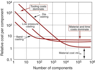
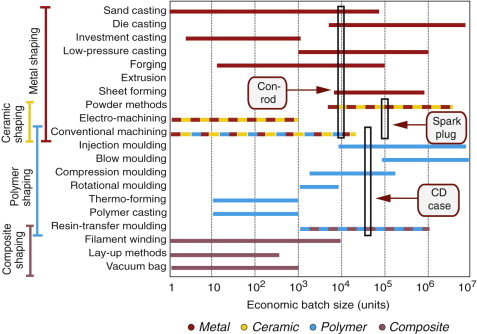
The crossover means that the process that is cheapest depends on the batch size. This suggests the idea of an economic batch size—a range of batches for which each process is likely to be the most competitive. Equation (18.6) allows the cost of competing processes to be compared if data for the parameters of the model are known. If they are not, the simpler economic batch size provides an alternative way of ranking. Figure 18.17 is a bar chart of this attribute, for the same processes and using the same colour coding as the earlier charts. Processes such as investment casting of metals and lay-up methods for composites have low tooling costs but are slow; they are economic when you want to make a small number of components but not when you want a large one. The reverse is true of the die casting of metals and the injection moulding of polymers: they are fast, but the tooling is expensive.
18.8 Computer-aided process selection
Computer-aided selection
As with the material charts, the process charts of this chapter give an overview, but the number of processes that can be shown on any one of them is limited. Selection using them is practical when there are few constraints, but when there are many—as there usually are—checking that a given process meets them all is cumbersome, and the cost model cannot be presented in a useful way because of the need for user-defined parameters. All these problems are overcome in the CES implementation of the method.
Its database contains records for processes, organised into the families, classes and members shown in Figures 2.5–2.7 of Chapter 2. Each record contains attribute data for a process, with each attribute stored as a range spanning its usual values, and is linked to the records for the materials it can process. It also contains limited documentation in the form of text, images and references to sources of information about the process. The data are interrogated by the same search engine that is used for material selection, allowing superimposed stages like those suggested by Figure 18.18. On the left is a stage that limits the process choice to those able to handle a chosen material family, class or member (here, thermoplastics). In the centre is a simple query interface for screening on one or more process attributes; the desired upper or lower limits for constrained attributes are entered and the search engine rejects all processes with attribute values that do not lie within the limits. On the right is a bar chart, constructed by the software, for any numeric attribute (here, economic batch size). For screening, a selection box is superimposed on the bar chart with upper and lower edges that lie at the constrained values of the attribute. This retains the processes with values that penetrate the box, rejecting those that lie outside it.
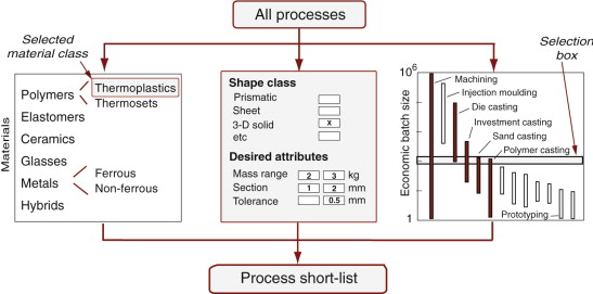
Figure 18.18 Schematic of the screening steps in selecting process (here for shaping). First specify classes such as material and shape; then screen on numeric attributes, plotted graphically to the right as bar charts. In the CES software, target design requirements can also be entered through dialog boxes, shown in the centre.
The software includes the batch-process cost model described in the text. A dialog box allows the user to edit default values of the user-defined parameters L, two, ![]() and so forth. The software then retrieves approximate values for the economic process attributes Cc, Ct,
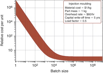
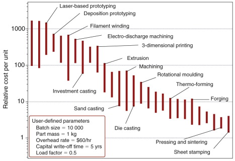
and so forth. The software then retrieves approximate values for the economic process attributes Cc, Ct, ![]() from the database where they are stored as ranges. It allows the data to be presented in a number of ways, two of which are shown in Figures 18.19 and 18.20. The first is a plot of cost against batch size for a single process (here, injection moulding), in the manner of the earlier Figure 18.16. The user-defined parameters are listed on it. The bandwidth derives from the ranges of the economic attributes: a simple shape, requiring only simple dies, lies near the lower edge; a more complex one, requiring multipart dies, lies near the upper edge. Figure 18.20 shows an alternative presentation. Here the range of cost for making a chosen batch size (here, 10 000) of a component by a number of alternative processes is plotted as a bar chart. The user-defined parameters are again listed. Other selection stages can be applied in parallel with this one (as in Figure 18.18) applying constraints on material, shape and so on, causing some of the bars to drop out. The effect is to rank the surviving processes by cost.
from the database where they are stored as ranges. It allows the data to be presented in a number of ways, two of which are shown in Figures 18.19 and 18.20. The first is a plot of cost against batch size for a single process (here, injection moulding), in the manner of the earlier Figure 18.16. The user-defined parameters are listed on it. The bandwidth derives from the ranges of the economic attributes: a simple shape, requiring only simple dies, lies near the lower edge; a more complex one, requiring multipart dies, lies near the upper edge. Figure 18.20 shows an alternative presentation. Here the range of cost for making a chosen batch size (here, 10 000) of a component by a number of alternative processes is plotted as a bar chart. The user-defined parameters are again listed. Other selection stages can be applied in parallel with this one (as in Figure 18.18) applying constraints on material, shape and so on, causing some of the bars to drop out. The effect is to rank the surviving processes by cost.
18.9 Case studies
Here we have examples of the selection methodology in use. In each case, translation of the design requirements leads to a target list of process attributes for screening. Three shaping problems are approached using the charts of this chapter, with the cost model applied to the last of the three. These are followed by examples of selecting joining and surface treatment processes. For these we use the CES software; the charts show only the broad classes of joining and finishing processes, whereas the level of detail in the software is much greater. In each case, aspects of processing beyond the scope of simple screening are noted. These relate to defects, or material properties, or economic limitations—all of which can be addressed by seeking documentation.
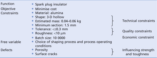
Shaping a ceramic spark plug insulator
The anatomy of a spark plug is shown schematically in Figure 18.21. It is an assembly of components, one of which is the insulator. This is to be made of a ceramic, alumina, in an axisymmetric, hollow 3-D shape. The insulator is part of an assembly, fixing its dimensions. Given the material and dimensions, the expected mass can be estimated and the minimum section thickness identified. The insulator must seal within its casing, setting limits on precision and surface finish. Spark plugs are made in large numbers—the projected batch size is 100 000. Table 18.5 lists the constraints. The lower part of the table flags up key process-sensitive outcomes that cannot be checked by screening, but should be investigated by a documentation search for the processes that successfully pass the screening steps.
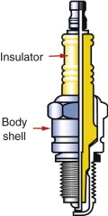
Figure 18.21 A section through a spark plug. The insulator is cylindrical but not prismatic, making it 3-D hollow in the shape classification.
Table 18.5 Translation for shaping a spark plug insulator and potential process-sensitive defects
|
The constraints are plotted on the compatibility matrices and bar charts of Figures 18.2–18.4, 18.11 and 18.12. The material compatibility chart shows only three process groups for ceramics, and all three can handle the required shape. All three can cope with the mass and the section thickness. All three can also meet the quality constraints on roughness and tolerance, although powder methods are near their lower limit. The constraint on economic batch size (Figure 18.17) identifies powder methods as the preferred choice. Applying the same steps using the CES software (Exercise E18.8) identifies two specific variants of powder methods that meet the constraints, listed in Table 18.6. Powder injection moulding is indeed the process used to make spark plug insulators.
Table 18.6 Short-list of processes for shaping a spark plug insulator
A documentation search details good practice in die design, powder quality, die filling and the cycle of pressure and temperature important for controlling porosity, finish and production rate.
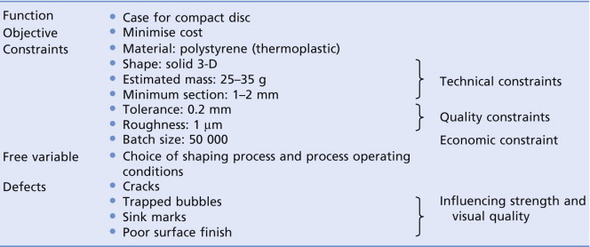
Shaping a thermoplastic CD case
The unsatisfactory qualities of the ‘jewel’ cases of CDs were noted in Chapter 3 and Figure 3.8. The current material choice is polystyrene, but before considering a change of material we might wish to check our processing options for thermoplastics in this geometry. Table 18.7 shows the translation for the CD case. The dimensions and mass are set by the standardised size of CDs. The shape is specified as ‘solid, 3-D’ as it is not a flat panel but has features at the edges to make the hinges and tabs to hold the sleeve in place. These features also require a good tolerance. Low surface roughness is needed to preserve transparency. We assume a target batch size of 50 000.
Table 18.7 Translation for shaping a CD case and potential process-sensitive defects
|
Refer again to the compatibility matrices and bar charts. Screening on the material (thermoplastic), shape, mass and minimum section leads to three possible processes: machining, injection moulding and compression moulding. Compression moulding is just beyond its normal mass range. All three processes meet the targets for tolerance and roughness. The final bar chart shows that machining is not economic for the given batch size, but the other two are acceptable. Table 18.8 summarises the surviving processes.
Table 18.8 Short-list of processes for shaping a polymer CD case
Good die design to include the protruding ridges and tabs on a CD case requires expert input. These re-entrant features exclude compression moulding using uniaxial loading and open dies. Following up the avoidance of defects, a documentation search is principally a matter of good die design with correct location of the runners and risers.
Shaping a steel connecting rod
Figure 18.22 shows a schematic connecting rod (‘con-rod’) to be made of a medium carbon steel. The minimum section is around 8 mm, and an estimate of the volume gives a mass around 0.35 kg. Dimensional precision is important to ensure clearances at both the little and the big end. The con-rod carries cyclic loads with the consequent risk of fatigue crack initiation, so a low surface roughness overall is necessary (the bores will be finished by a subsequent machining operation). A modest batch size of 10 000 is required. Control of properties and of defects is dominated by the need to avoid fatigue failure. Table 18.9 summarises.
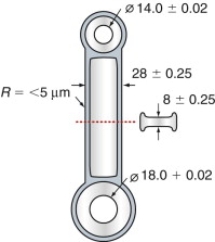
Figure 18.22 A steel connecting rod. The precision required for the bores and bore facing is much higher than for the rest of the body, requiring subsequent machining. Dimensions in µm (unless otherwise stated).
Table 18.9 Translation for shaping a steel connecting rod and potential process-sensitive defects

|
These constraints are plotted on the matrices and charts. Screening on material and shape eliminates low-pressure casting, die casting, extrusion and sheet forming, but plenty of options survive. Sand casting is disqualified by the tolerance constraint. Investment casting, conventional machining, forging and powder methods remain. All achieve the target roughness, and surface tolerance, though not that required for the bores. However, by following the shaping process with a finishing process, the tolerance requirement can be reached. All the finishing processes at the bottom of Figure 18.11 give better tolerance and roughness than specified—precision machining is most appropriate for finishing the bores and the faces surrounding them. Finally, the economic batch size chart suggests that forging and powder methods are suitable—machining (from solid) and investment casting are not economic for a batch size of 10 000. Table 18.10 summarises.
Table 18.10 Short-list of processes for shaping a steel connecting rod
This case study reveals that there is close competition for the manufacture of carbon steel components in the standard mid-range size and shape of a connecting rod. Surface finish and accuracy present some problems, but finishing by machining is not difficult for carbon steel. The final choice will be determined by detailed cost considerations and achieving the required fatigue strength. The properties will be sensitive to the composition of the steel and its heat treatment—something illustrated further in the next chapter.
Cost is considered further by applying the model of Section 18.7. Table 18.11 lists values for the parameters in the cost model for three processes: die casting, forging and powder methods. Assuming the same amount of material is used in each process, the costs are all normalised to the material cost. Figure 18.23 shows the computed relative cost per part against batch size for the three processes.
Table 18.11 Process cost model input data for three shaping methods to make the con-rod
| Parameters | Die casting | Forging | Powder methods |
|---|---|---|---|
| *Material, mCm/(1 − f) | 1 | 1 | 1 |
| *Basic overhead, |
100 | 100 | 100 |
| Capital write-off time, two (years) | 5 | 5 | 5 |
| Load factor | 0.5 | 0.5 | 0.5 |
| *Dedicated tooling cost, Ct | 17 500 | 125 | 1000 |
| *Capital cost, Cc | 50 000 | 110 000 | 1 000 000 |
| Production rate, |
50 | 50 | 2 |
* Costs normalised to mCm/(1 − f).
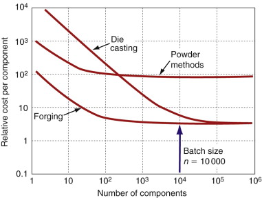
Figure 18.23 The cost model for three possible processes to manufacture the steel con-rod, using representative constant values for the model parameters. For the target batch size of 10 000, the cheapest option indicated is forging.
For the batch size of 10 000 forging comes out the cheapest, followed closely by die casting. Powder is more expensive, principally because the slower production rate and high capital cost give a large overhead contribution per part. Since there is a spread of estimated cost (due to uncertainty in the inputs), and forging is likely to be followed by machining, the cost difference between forging and die casting is not significant—both remain on the list for investigation of the achievable properties.
Joining a steel radiator
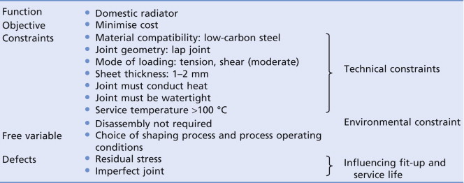
Figure 18.24 shows a section through a domestic radiator made from corrugated pressed sheet steel. The task is to choose a joining process for the seams between the sheets. As always, the process must be compatible with the material (here, low-carbon steel sheet of thickness 1.5 mm). The lap joints carry only low loads in service but handling during installation may impose tension and shear. They must conduct heat, be watertight and be able to tolerate temperatures up to 100 °C. There is no need for the joints to be disassembled for recycling at the end of life, since the whole thing is steel. Quality constraints are not severe, but distortion and residual stress will make fit-up of adjacent joints difficult. Low carbon steels are readily weldable, so it is unlikely that there is a risk of any welding process causing cracking or embrittlement problems—but this can be checked by seeking documentation. Table 18.12 summarises the translation.
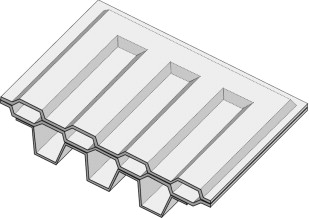
Figure 18.24 A section through a domestic radiator. The three pressed steel sections are joined by lap joints.
Table 18.12 Translation for joining a steel radiator and outcome (potential process-sensitive defects and properties)
|
To tackle this selection we use the Cambridge Engineering Selector. It stores records and attributes for 52 joining processes. Applying the material compatibility check first, 32 processes are found to be suitable for joining low-carbon steel—those eliminated are principally polymer-specific processes. Further screening on joint geometry, mode of loading and section thickness reduces the list to 20 processes. The requirement to conduct heat is then the most discriminating—only 10 processes now pass. Water resistance and operating temperature do not change the short-list further. The processes passing the screening stage are listed in Table 18.13.
Table 18.13 Short-list of processes for joining a steel radiator
Quality and economic criteria are difficult to apply as screening steps in selecting joining processes. At this point we seek documentation for the processes. This reveals that explosive welding requires special facilities and permits (hardly a surprise). Electron beam and laser welding require expensive equipment, so use of a shared facility would be necessary to make them economic. Resistance spot welding is screened out because it failed the requirement to be watertight. This is only necessary for the edge seams, so internal joint lines could be spot welded. This highlights the need for judgement in applying automated screening steps. Always ask: has an obvious (or existing) solution been eliminated? Why was this? Has something narrowly failed, so that a low-cost option could be accommodated with modest redesign? Could a second process step, like sealing the spot-welded joint with a mastic, correct a deficiency? The best way forward is to turn constraints on and off, and adjust numerical limits, exploring the options that appear.
Surface hardening a ball bearing race
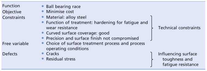
The balls of ball bearing races run in grooved tracks (Figure 18.25). As discussed in Chapter 11, the life of a ball race is limited by wear and by fatigue. Both are limited by using hard materials. Hard materials, however, are not tough, incurring the risk that shock loading or mishandling might cause the race to fracture. The solution is to use an alloy steel, which has excellent bulk properties, and to apply a separate surface treatment to increase the hardness where it matters. We therefore seek processes to surface harden alloy steels for wear and fatigue resistance. The precision of both balls and race is critical, so the process must not compromise the dimensions or the surface smoothness. Table 18.14 summarises the translation.
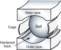
Figure 18.25 A section through a ball bearing race. The surface of the race is to be hardened to resist wear and fatigue crack initiation.
Table 18.14 Translation for surface hardening a ball bearing race and potential process-sensitive defects
|
The CES system contains records for 44 surface treatment processes. Many are compatible with alloy steels. More discriminating is the purpose of the treatment—to impart fatigue and wear resistance—reducing the list to eight. Imposing the requirement for a very smooth surface knocks out those that coat or deform the surface because these compromise the finish. The short-list of processes that survive the screening is given in Table 18.15. Adding the further constraint that the curved surface coverage must be very good leaves just the first two: carburising and carbonitriding, and nitriding.
Table 18.15 Short-list of processes for hardening an alloy steel ball race
To get further we turn to documentation for these processes. The hardness of the surface and the depth of the hardened layer depend on process variables: the time and temperature of the treatment and the composition of the steel. And economics, of course, enters. Ball races are made in enormous batches and although their sizes vary, their geometry does not. This is where dedicated equipment, even if very expensive, is viable.
18.10 Summary and conclusions
Selecting a process follows a strategy much like that for materials: translation of requirements, screening of the options, ranking of the processes that survive screening, ending with a search of documentation for the most promising candidates. For processes, translation is straightforward—the requirements convert directly into the attributes of the process to be used in the screening step. Process attributes capture their technical capabilities and aspects of product quality. All process families require screening for compatibility with material to which they are to be applied, but after this the attributes and constraints are specific to the family. For shaping, component geometry, precision and finish are most discriminating. For joining it is joint shape and mode of loading. For surface treatments it is the purpose for which the treatment is applied (wear, corrosion, aesthetics, etc.). Ranking is based on cost if this can be modeled, as it can for batch processes. Cost models combine characteristic process attributes such as tooling and capital costs and the production rate, with user-specified parameters such as overhead rates and required batch size. The economic batch size provides a crude alternative to the cost model—a preliminary indication of the batch size for which the process is commonly found to be economic.
Translation of the design requirements frequently points to important aspects of processing that fall beyond a simple screening process. The avoidance of defects, achieving the required modification of material properties and determining the process speed (and thus economics), all involve coupling between the process operating conditions, the material composition and design detail. This highlights the importance of the documentation stage in making the final choice of processes, and the need to refine the material and process specifications in parallel. The next chapter explores aspects of process-property interactions in more depth.
Ashby M.F. Materials Selection in Mechanical Design 3rd ed. 2005 Butterworth-Heinemann Oxford, UK Chapter 4. ISBN 0-7506-6168-2. (The source of the process selection methodology and cost model, with further case studies, giving a summary description of the key processes in each class.)
ASM Handbook Series ASM Handbook Series (1971–2004). Volume 4, Heat Treatment; Volume 5, Surface Engineering; Volume 6, Welding, Brazing and Soldering; Volume 7, Powder Metal Technologies; Volume 14, Forming and Forging; Volume 15, Casting; and Volume 16, Machining; ASM International, Metals Park, OH, USA. (A comprehensive set of handbooks on processing, occasionally updated, and now available online at www.asminternational.org/hbk/index.jsp
Bralla J.G. Design for Manufacturability Handbook 2nd ed. 1998 McGraw-Hill New York, USA ISBN 0-07-007139-X. (Turgid reading, but a rich mine of information about manufacturing processes.)
Campbell J. Casting 1991 Butterworth-Heinemann Oxford, UK ISBN 0-7506-1696-2. (The fundamental science and technology of casting processes.)
Houldcroft P. Which Process? 1990 Abington Publishing Abington, Cambridge, UK ISBN 1-85573-008-1. (The title of this useful book is misleading—it deals only with a subset of joining process: the welding of steels. But here it is good, matching the process to the design requirements.)
Kalpakjian S., Schmid S.R. Manufacturing Processes for Engineering Materials 4th ed. 2003 Prentice-Hall, Pearson Education New Jersey, USA ISBN 0-13-040871-9. (A comprehensive and widely used text on material processing.)
Lascoe O.D. Handbook of Fabrication Processes 1988 ASM International, Metals Park Columbus, OH, USA ISBN 0-87170-302-5. (A reference source for fabrication processes.)
Swift K.G., Booker J.D. Process Selection, from Design to Manufacture 1997 Arnold London, UK ISBN 0-340-69249-9. (Details of 48 processes in a standard format, structured to guide process selection.)
18.12 Exercises
- Exercise E18.1
- (a) Explain briefly why databases for initial process selection need to be subdivided into generic process classes, whereas material selection can be conducted on a single database for all materials.
- (b) After initial screening of unsuitable processes, further refinement of the process selection usually requires detailed information about the materials being processed and features of the design. Explain why this is so, giving examples from the domains of shaping, joining and surface treatment.
- Exercise E18.2 A manufacturing process is to be selected for an aluminum alloy piston. Its weight is between 0.8 and 1 kg, and its minimum thickness is 4–6 mm. The design specifies a precision of 0.5 mm and a surface finish in the range 2–5 µm. It is expected that the batch size will be around 1000 pistons. Use the process attribute charts earlier in the chapter to identify a subset of possible manufacturing routes, taking account of these requirements. Would the selection change if the batch size increased to 10 000?
Exercise E18.3 The choice of process for shaping a CD case was discussed in Section 18.5, but what about the CDs themselves? These are made of polycarbonate (another thermoplastic), but the principal difference from the case is precision. Reading a CD involves tracking the reflections of a laser from microscopic pits at the interface between two layers in the disc. These pits are typically 0.5 µm in size and spacing, and 1.5 µm apart; the tolerance must be better than 0.1 µm for the disc to work.
First estimate (or measure) the mass and thickness of a CD. Use the charts to find a short-list of processes that can meet these requirements, and will be compatible with the material class. Can these processes routinely achieve the tolerance and finish needed? See if you can find out how they are made in practice.
18.13 Exploring design with CES
- Exercise E18.4 Use the ‘Browse’ facility in CES to find:
- (a) The record for the shaping process injection moulding, thermoplastics. What is its economic batch size? What does this term mean?
- (b) The machining process water-jet cutting (records for machining processes are contained in the Shaping data table). What are its typical uses?
- (c) The joining process friction-stir welding. Can it be used to join dissimilar materials?
- (d) The surface treatment process laser hardening. What are the three variants of this process?
- Exercise E18.5 Use the ‘Search’ facility in CES to find:
- Exercise E18.6 Use CES Level 3 to explore the selection of casting process for the products listed. First check compatibility with material and shape, and make reasonable estimates for the product dimensions (to assess mass and section thickness). Then include appropriate values for tolerance, roughness, and economic batch size.
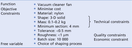
Exercise E18.7 A small nylon fan is to be manufactured for a vacuum cleaner. The design requirements are summarised in the following table. Use CES Level 3 to identify the possible processes, making allowance if necessary for including a secondary finishing process. Suggest some aspects of the design that may merit investigation of supporting information on the selected processes.
Exercise E18.8 The selection of process for a connecting rod was discussed earlier in the chapter. Conduct the selection using CES Level 3, making reasonable estimates for any unspecified requirements. Explore the effect of changing to a 3 m con-rod for a ship, of approximate cross-section 10 × 10 cm, in a batch size of 10.
- Exercise E18.9 Process selection for an aluminum piston was investigated in Exercise E18.2. Further investigation of the economics of gravity die casting and ceramic mould casting is suggested. Plot the cost against batch size for these processes, assuming a material cost of $2/kg and a piston mass of 1 kg. The overhead rate is $70/hour, the capital write-off time is 5 years and the load factor is 0.5. Which process is cheaper for a batch size of 1000? Assume that as the piston is simple in shape, it will fall near the bottom of each cost band.
- Exercise E18.10 Two examples of selection of secondary processes were discussed in this chapter. The design requirements were summarised for joining processes for a radiator in Table 18.12 and for hardening a steel bearing race in Table 18.14. Use CES Level 3 to check the results obtained. For the radiator problem, use the ‘Pass–Fail table’ feature in CES to see if other processes could become options if the design requirements were modified.
18.14 Exploring the science with CES Elements
- Exercise E18.11 Casting processes require that the metal be melted. Vapour methods like vapour metallising require that the metal be vapourised. Casting requires energy: the latent heat of melting is an absolute lower limit (in fact it requires more than four times this). Vapourisation requires the latent heat of vapourisation, again as an absolute lower limit. Values for both are contained in the Elements database. Make a plot of one against the other. Using these lower limits find, approximately, how much more energy-intensive vapour methods are compared with those that simply melt.