
Chapter 19 Follow the recipe: Processing and properties
- 19.1 Introduction and synopsis 460
- 19.2 Processing for properties 461
- 19.3 Microstructure of materials 463
- 19.4 Microstructure evolution in processing 466
- 19.5 Metals processing 479
- 19.6 Non-metals processing 493
- 19.7 Making hybrid materials 496
- 19.8 Summary and conclusions 499
- 19.9 Further reading 500
- 19.10 Exercises 500
- 19.11 Exploring design with CES 502
Some people are better at multi-tasking than others. The good ones should feel at home in manufacturing. Shaping, finishing and assembling components into products to meet the technical, economic and aesthetic expectations of consumers today requires the balancing of many priorities. Earlier chapters have introduced intrinsic properties—strength, resistivity and so on—that depend intimately on microstructure, and microstructure depends on processing. Microstructure is not accessible to observation during processing, so controlling it requires the ability to predict how a given process step will cause it to evolve or change. So manufacturers have their work cut out to turn materials reliably into good-quality products, while making themselves a decent profit. Manufacturing involves more than making materials into the right shapes and sticking them together; it is also responsible for producing properties on target.
19.1 Introduction and synopsis
Some people are better at multi-tasking than others. The good ones should feel at home in manufacturing. Shaping, finishing and assembling components into products to meet the technical, economic and aesthetic expectations of consumers today requires the balancing of many priorities. Earlier chapters have introduced intrinsic properties—strength, resistivity and so on—that depend intimately on microstructure, and microstructure depends on processing. Microstructure is not accessible to observation during processing, so controlling it requires the ability to predict how a given process step will cause it to evolve or change. So manufacturers have their work cut out to turn materials reliably into good-quality products, while making themselves a decent profit. Manufacturing involves more than making materials into the right shapes and sticking them together; it is also responsible for producing properties on target.
There is a parallel with cooking. The recipe lists the ingredients and cooking instructions: how to mix, beat, heat, finish and present the dish. A good cook draws on experience (and creativity) to produce new dishes with pleasing flavour, consistency and appearance; you might think of these as the attributes of the dish. But if the dish is not a success the first thing the cook might do is to cut right through it and examine what went wrong with its microstructure. Suppose, for instance, the dish is a fruit cake, then the distribution of porosity and fruit constitutes aspects of its microstructure.
Microstructure is key to engineering properties too. Some of its components are very small—precipitate particles can consist of clusters of a few atoms. Others are larger—grains range in size from microns to millimeters. The goal of this chapter is to explore how microstructures evolve during processing, with the focus on processing for properties. The ability to tune microstructure and properties is central to materials processing and design, so it brings with it the need for good process understanding and control. Failure to ‘follow the recipe’ leads, at best, to scrap and lost revenue and, at worst, to engineering failures. The essence of the chapter is therefore captured by the statement:
The chapter opens with an illustrative example—making an aluminum bicycle frame—to highlight some general features of processing for properties. Microstructural features were introduced in many previous chapters, in ‘drilling down’ into the underlying science, so these are drawn together in an overview across the length scales, for reference. In materials processing, the evolution of the microstructure is governed primarily by the thermal (and sometimes deformation) history. When drilling down in this context, particularly for metals, the central topics are phase diagrams and the thermodynamics and kinetics of phase transformations.
The main text of the chapter provides a concise overview of these topics. A detailed coverage of how to read and interpret phase diagrams, and the microstructural evolution in common processes, is provided in Guided Learning Unit 2, Phase Diagrams and Phase Transformations, for those seeking more depth. A wide range of manufacturing processes for metals and non-metals are then considered. In each case process schematics explain how the process works, highlighting the key role of thermal history and cooling rate in determining the microstructure evolution. As in earlier chapters, property charts are used to illustrate the property changes imparted by composition and processing, with examples from each of the material classes.
19.2 Processing for properties
We noted earlier that the mantra for this chapter is: Composition + Processing → Microstructure + Properties. So here is an example to highlight some general issues about this interaction.
Aluminum bike frames
The material chosen for our illustrative bike frame example is a heat-treatable aluminum alloy, for its good stiffness and fatigue resistance at low weight (Chapters 5 and 10). Figure 19.1 illustrates the main steps in the process history. It makes a number of points.
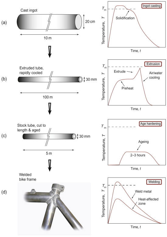
Figure 19.1 A schematic process history for the manufacture of a bike frame in heat-treatable aluminum alloy: (a) casting of large ingot, cut into billets for extrusion; (b) hot extrusion into tube, incorporating the solution heat treatment and quench; (c) sections cut to length and age hardened; (d) assembly into the frame by arc welding.
Point 1: Materials processing involves more than one step. This bike frame is an example of a wrought product (i.e. one that undergoes some deformation processing) involving a chain of processes. In contrast, shaped metal casting, powder processes and polymer moulding are near-net-shape processes—the raw material is turned into the shape of the component in a single step, leaving only finishing operations (including heat treatment), so the number of steps is lower. Wrought alloys start life as a casting, but this ingot casting is most economic on a large scale, as in Figure 19.1(a). Standard compositions are cast in large plant, and transported to different factories for processing into different products. For the bike frame, the ingot is sliced into billets and extruded into tube, as in Figure 19.1(b). It is shaped directly from a solid circular billet, around 200 mm in diameter, to a hollow tube, 30 mm in diameter and 3 mm thick—a huge shape change in one step. The tube is then cut to length before the final stages of age hardening for optimum strength and assembly by arc welding (Figure 19.1(c) and (d)). In passing, we note that the composition of the chosen alloy must be adjusted at the outset, via processing in the liquid state. It cannot be changed after casting (other than at the surface). Metallic elements dissolve freely in one another in the liquid state, but it is very difficult to add them in the solid state; diffusion is much too slow.
Point 2: Each process step has a characteristic thermal history. Each temperature cycle is determined by the way the process step works, and what the target outcome is. Casting by definition involves melting, solidification and cooling. Extrusion is done hot to reduce the strength and to increase the ductility. This enables the material to undergo the large plastic strain, allowing fast throughput at relatively low extrusion force. The quality of surface finish is also determined at this stage. At the same time, extrusion enhances the microstructure. Hot deformation refines the grain structure in the as-cast billet, and helps to homogenise the alloy. Then as the tube emerges from the extrusion press, forced cooling quenches it to trap solute elements in solid solution, thus avoiding the need for a subsequent solution heat treatment (the first step of age hardening a heat-treatable aluminum alloy). In a non-heat-treatable aluminum alloy, strength comes from solid solution and work hardening, not precipitation, so the extrusion is often done cold to maximise the work hardening, without a further heat treatment. Note therefore the interplay between deformation and thermal histories, and how this is critical for controlling the shape and final properties simultaneously, while the detail depends on the particular alloy variant being processed.
Point 3: Designers should watch out for unintended side-effects in the joining stage. Bike frame assembly here is by arc welding, with its own temperature cycle back to the melting point. In the ‘heat-affected zone’ around the welds the alloy doesn’t melt, but is hot enough for the microstructure to evolve—the precipitates carefully produced by prior age hardening can disappear back into solution. As the whole age-hardening cycle is difficult to repeat on the completed frame, the heat-affected zone ends up with different, inferior properties to the rest of the frame (discussed further in Section 19.5).
Point 4: Design focuses on the properties of finished products, but some of these properties (strength, ductility, thermal conductivity, etc.) are also critical during processing. And there are other properties that are only really relevant for processing—for example, the viscosity of the melt in metal casting or polymer moulding. Design and processing characteristics can often be in conflict—strong alloys are more difficult to process and are thus more expensive. So in choosing materials for a component it is important to examine their suitability for processing as well as for performance in service. Clever processing tricks are exploited to resolve the conflicts—the bike frame is hot-formed (when it is soft) and then heat-treated (after shaping) to produce the high strength for service.
This introductory example shows how combinations of chemistry and processing are used to manipulate microstructure and properties. Further examples are given later for all material classes. The goal is to understand the interactions between processing and the target ‘ideal’ properties, as stored in a property database. But the bicycle frame case study shows that we need to keep our eyes open in this game, and to be aware that we often have to compromise between design objectives and manufacturing realities, and that things can go badly wrong. The importance of the ‘Seek Documentation’ stage in material and process selection should not be underestimated!
19.3 Microstructure of materials
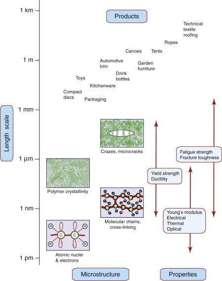
Before exploring what goes on inside materials in a range of processes, it is helpful to see the ‘big picture’ in relation to microstructure. Properties reflect microstructure from atoms to grains to cracks, spanning length scales over many orders of magnitude. Here we draw together all of the microstructural features introduced earlier in the book, by way of an overview.
Metals
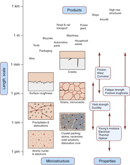
Figure 19.2 summarises the main microstructural features in metals. Starting at the bottom with atoms, we have crystalline packing (with the exception of the unusual amorphous metals)—responsible for elastic moduli and density. Atom-scale defects—vacancies and solute atoms—were introduced in Chapter 6. Thermal, electrical, optical and magnetic behaviour are most directly influenced by this atomic scale of microstructure. Vacancies are responsible for diffusion so this, and the service and processing phenomena it causes (creep, sintering, heat treatments), also depend on atomic-scale structure. Strength, toughness and fatigue depend on structure at a slightly larger scale, that of dislocations and the obstacles to their motion sketched in Figure 19.2: precipitates and grain boundaries. Grains themselves usually fall into the 1–50 µm scale—a similar scale to the roughness on metal surfaces and of the porosity caused by the gasses trapped in a metal when it is cast. Fatigue cracks start at grain scale, but grow to the dimensions of the component itself at fracture. Metal products themselves span a huge range: kitchen foil is around 10 µm thick, automotive panels a millimetre or so, ship propellers are several metres in diameter, and bridges and buildings reach the kilometre scale.
Ceramics and glasses
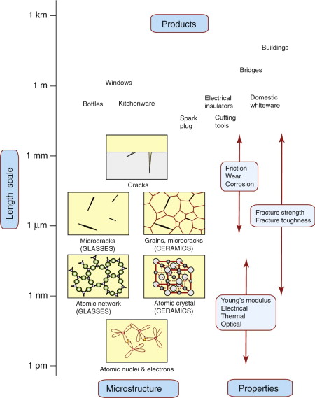
Ceramics are crystalline, glasses are amorphous. Figure 19.3 shows both near the bottom of our materials length scale. Most of the properties directly reflect the atomic layout and the intrinsically strong nature of the covalent or ionic bonding—from elastic modulus to electrical insulation. Atomic scales also govern viscosity in molten glass and diffusion in compacted ceramic powders. The exceptions are strength and toughness. Cracks dominate failure in ceramics and glasses, so these are the key features—closely related to grain size (in ceramics) and to the surface finish.
Polymers and elastomers
Polymers and elastomers are inherently molecular rather than atomic. Figure 19.4 shows that there is wide diversity at this fine scale: polymer molecules can be amorphous, crystalline, cross-linked or aligned by drawing. Most properties again reflect behaviour at this scale, with strength and toughness (and optical properties) bringing in larger features such as crazes and cracks. Polymer foams and fibre-reinforced polymer composites have additional length scales relating to their architecture—for example, pore size and fibre diameter. These and other ‘hybrid’ materials are discussed further in Section 19.7.
19.4 Microstructure evolution in processing
The role of shaping processes is to produce the right shape with the right final properties. Achieving the first requires control of viscous flow or plasticity. Achieving the second means control of the nature and rate of microstructural evolution. Secondary processing (joining and surface treatment) may cause the structure to evolve further. Examples of microstructural evolution are discussed in Sections 19.5 and 19.6, but first some general principles on why and how it happens. The emphasis is on metals, reflecting their great diversity in both alloy chemistry and process variants.
Phase diagrams, phase transformations and other structural change
A phase is defined as a region of a material with a specified atomic arrangement. This means that a phase has characteristic physical properties, such as density. Steam, water and ice are the vapour, liquid and solid phases of H2O. Engineering alloys such as steel also melt and then vapourise if we heat them enough. More interestingly, they can contain different phases simultaneously in the solid state, depending on the composition and temperature. It is this that gives us precipitation-hardened steels and non-ferrous alloys, made up of one phase, the precipitate, in a matrix of the other. The precipitates may contain only a handful of atoms, but they are nonetheless a separate single phase with a defined crystallographic structure.
Phase diagrams are essential tools of the trade for processing of metals and ceramics: they are maps showing the phases expected as a function of composition and temperature, if the material is in a state of thermodynamic equilibrium. By this we mean the state of lowest free energy (defined in more detail later), such that there is no tendency to change.
A phase transformation occurs when the phases present change—for example, melting of a solid, solidification of a liquid, or a solid solution forming a dispersion of fine precipitates within a crystal. Phase diagrams show us when changes such as these are expected as the temperature rises and falls. Phase transformations are thus central to microstructural control in metal processing.
A change in the phases present requires a driving force and a mechanism. The first is determined by thermodynamics, the second by kinetic theory. The term driving force, somewhat confusingly, actually means a change in free energy between the starting point (the initial phase or phases) and the end point (the final state). A ball released at the top of a ramp will roll down it because its potential energy at the bottom is lower than that at the top. Here the driving force is the potential energy. Phase changes are driven by differences in free energy—solids melt on heating because being a liquid is the state of lowest free energy above the melting point. And chemical compounds can have lower free energy than solid solutions, so an alloy may decompose into a mixture of phases (both solutions and compounds) if, in so doing, the total free energy is reduced.
Microstructures can therefore only evolve from one state to another if it is energetically favourable to do so—thermodynamics points the way for change. But having energy available is not sufficient in itself to make the change happen. Changes in microstructure also need a mechanism for the atoms to rearrange from one structure to another. For example, when a liquid solidifies, there is an interface between the liquid and the growing solid. This is where kinetic theory comes in—atoms transfer from liquid to solid by diffusion at the interface. Virtually all solid-state phase changes also involve diffusion to move the atoms around to enable new phases to form. Diffusion occurs at a rate that is strongly dependent on temperature—we calculated it in Chapter 13. The overall rate of structural evolution depends on both the magnitude of the driving force (no driving force, no evolution) and the kinetics of the diffusion mechanism by which it takes place. The rates of structural evolution are of great significance in processing. First they govern the length scale of the important microstructural features—grains, precipitates and so on—and thus the properties. But they also affect process economics, via the time it takes for the desired structural change to occur.
Solidification and precipitation involve changes in the phases present. There are other important types of structure evolution in processing that do not involve a phase change, but the principles are the same: there must be a reduction in energy, and a kinetic mechanism, for the change to occur. Concentrated solid solutions have higher free energy than dilute ones, so gradients in concentration tend to smooth out, if heated to give the solute atoms enough diffusive mobility. Recovery and recrystallisation are mechanisms that change the grain structure of a crystal, even though the phases making up the grains do not change. The driving force comes from the stored elastic energy of the dislocations in a deformed crystal, released as the density of dislocations falls; the mechanism of recrystallisation is diffusive transfer of atoms across the interface between the deformed and new grain structures. We revisit these examples later in the chapter, in relation to manufacturing processes in which they occur.
Thermodynamics of phases
Materials processing principally deals with liquids and solids—only a few special coating processes deal with gasses (for example, vapour deposition onto a substrate). Drilling down into the origins of material properties in earlier chapters, we have seen that solid phases can form as pure crystals of a single element, as solid solutions of two or more elements, or as compounds with well-defined crystal structure and stoichiometry (by which we mean the relative proportions of the different elements are simple integers: alumina Al2O3, iron carbide Fe3C and so on).
So if we take an alloy of a given composition and hold it at a fixed temperature, what determines whether it will be solid, liquid or a mixture of the two? Or a solid solution, a compound or a mixture of solid phases? The answer lies in thermodynamic equilibrium and the Gibbs1 free energy, G, defined as
The thermodynamic variables in this equation require some explanation. The internal energy U is the intrinsic energy of the material associated with the chemical bonding between the atoms and their thermal vibration. We have encountered it before in the cohesive energy responsible for recoverable elastic strain and stored energy under load (Chapter 4), or thermal expansion (Chapter 12). The pressure p, volume V and temperature T are the thermodynamic state variables familiar from the universal gas law. The combination U + pV is so common that it is frequently combined as the enthalpy, H. In materials processing, we are concerned mostly with changes in free energy rather than absolute values. Pressure is usually at or close to atmospheric, and volume changes in metals are modest in the liquid or solid state, so changes in enthalpy are usually dominated by the internal energy U.
Entropy S is a complex concept in thermodynamics associated with how exchanges of heat at a given temperature change the enthalpy of a system, and whether the exchange is reversible. This is central to determining the efficiencies of gas-based systems that generate and exchange heat to do mechanical work, such as internal combustion engines and gas turbines. For material phase changes, a common interpretation of entropy is as a measure of the disorder in the system. For a solid crystal to melt, heat must be supplied (at constant temperature) to overcome the intrinsic ‘latent heat’ of melting. We will see later that this is an enthalpy change, with a corresponding increase in the entropy. The rise in entropy is associated with the greater disorder in the liquid state, compared to the regular packed state of the solid. Changes in entropy of a crystalline solid are relatively small (due to the regular atomic packing). Entropy is much more important in polymers, since the molecules have more freedom to adopt different configurations.
So, for any composition and temperature we could (at least in principle) calculate the free energy of alternative material states—liquid solution, solid solution, mixtures of phases and so on. Out of the unlimited number of possible states, that with the lowest free energy is the state at thermodynamic equilibrium. Higher energy states may form, but there is then the possibility of energy being released by a change to equilibrium. Only at equilibrium is no change physically possible. In practical alloy processing it is often easy enough to reach equilibrium or near-equilibrium states—hence the importance of phase diagrams, which map the equilibrium phases expected for a given alloy.
Guided Learning Unit 2: phase diagrams and phase transformations (Parts 1–4)
Phase diagrams and phase transformations are big topics in process metallurgy. In the following subsections, we give a concise summary of phase diagrams and the underlying science of phase transformations. Guided Learning Unit 2 goes into depth on how to interpret phase diagrams and relate them to microstructural evolution in common processes. The rest of this chapter will be intelligible without diverting into the unit, but a more complete grasp is available by working through the Guided Learning text and exercises. It is recommended that Guided Learning Unit 2 is visited in two installments. Parts 1–4 cover phase diagrams and how to read them: work through this now. Parts 5–8 cover common phase transformations—you will be prompted in the text when it is best to go back to these sections.
Phase diagrams: illustrative examples
Real alloys can contain up to 10 or more different elements, though many contain only two. The starting point for understanding all alloys is to consider the principal element mixed with one other element, making a binary alloy (or system). Carbon steels are based on iron-carbon, stainless steels on iron-chromium and so on. Phase diagrams for binary alloys are plots of temperature against composition, showing the fields in which the equilibrium phase or phases are fixed. Figure 19.5 shows a simple example: the phase diagram for the binary lead-tin (Pb-Sn) system. This and more complex diagrams are built up and explained in more detail in Guided Learning Unit 2.
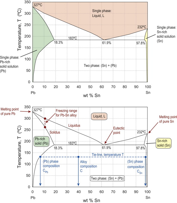
Figure 19.5 Phase diagram for the binary Pb-Sn system, showing a number of key features. In the upper figure, the single-phase fields are: liquid—peach; Pb-rich solid solution (Pb)—green; Sn-rich solid solution (Sn)—yellow. These are separated by two phase fields, the relevant phases being identified by a horizontal tie-line, as shown in the (Pb)–(Sn) field in the lower figure. Also shown are the melting points of the pure elements, the freezing range between liquidus and solidus boundaries for alloy compositions and the eutectic point at the bottom of the liquid field.
Note the following features of Figure 19.5:
- The diagram divides up into single- and two-phase regions, separated by phase boundaries.
- At any point in the two-phase regions, the phases present are those found at the phase boundaries at either end of a horizontal ‘tie-line’ through the point defining the composition and temperature concerned.
- Both Pb and Sn will dissolve one another to some extent (Sn is more soluble in Pb than the reverse), with the maximum solubility in both cases being at the same temperature.
- The pure elements (Pb and Sn) have a unique melting point (at which the material can change from 100% solid to 100% liquid).
- Alloys show a ‘freezing range’ between the boundaries known as the liquidus and solidus, so there is no longer a single melting point.
- At one special point, the eutectic, the alloy can change from 100% liquid to 100% two-phase solid at a fixed temperature (it is the only place at which three phases can co-exist); this temperature is the lowest temperature at which 100% liquid is possible.
The Pb-Sn system only contains solid solutions, and mixtures of the two. The common appearance of compounds on phase diagrams is illustrated in Figure 19.6, part of the aluminum-copper (Al-Cu) system. The compound CuAl2 contains one Cu atom for every two Al atoms: 33 atom % (at%) Cu. Converted to percentage by weight (see Guided Learning Unit 2), the compound is Al-53 wt% Cu. The phase diagram shows a thin vertical single-phase field for CuAl2. The small spread of composition shows that the stoichiometry need not be exactly in the 1:2 atomic ratio of Cu:Al, but some excess Al can be accommodated in the CuAl2 crystal structure. Most compounds show some spread in their composition, but some are strictly stoichiometric—the single-phase field appears as a vertical line on the diagram. Note that between pure Al and CuAl2, the form of the phase diagram is similar to the binary system in Figure 19.5, with a eutectic point at 33 wt% Cu.
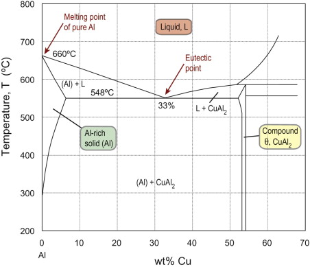
Figure 19.6 Phase diagram for part of the binary Al-Cu system, showing the compound CuAl2 at 53 wt% Cu.
Figure 19.7 shows the important Fe-C phase diagram. It too has a compound (iron carbide, Fe3C) and a eutectic point (at 4.3 wt% C and 1147 °C) but in other respects it is a bit more complicated, with a number of additional features (explained more fully in Guided Learning Unit 2):
- Pure iron shows three phases in the solid state: as the temperature increases iron changes from α-iron (BCC lattice) to γ-iron (FCC lattice) before reverting to BCC δ-iron and then melting.
- The single-phase austenite field (solid solution of carbon in FCC γ) has a eutectoid point at its base—at this point the single-phase austenite at a composition of 0.8 wt% C can transform on cooling to a mixture of ferrite (a solid solution of carbon in BCC α) and cementite (the compound Fe3C).
- The austenite field closes at the top in a peritectic point, at which single-phase austenite with this composition transforms on heating to a mixture of liquid and δ-iron.
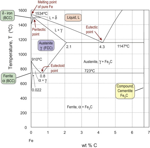
Figure 19.7 Phase diagram for part of the binary Fe-C system, up to the compound iron carbide (cementite) Fe3C at 6.7 wt% C. The single phases are: liquid, and 3 solid solutions of carbon in iron: α-iron (ferrite), γ-iron (austenite) and δ-iron. The Fe-C system contains a eutectic point, and the austenite field closes at the bottom with a eutectoid point, and at the top with a peritectic point.
As discussed in Guided Learning Unit 2 (Part 8), an important practical consequence of this diagram relates to heat treatments that exploit the difference in solubility of carbon in FCC and BCC iron.
Thermodynamics and kinetics of phase transformations
We noted earlier that the equilibrium state was that with the lowest free energy at a given composition and temperature. The boundaries on phase diagrams show where two different states can both be in equilibrium. So what happens if we start at equilibrium in one field of the diagram and change the temperature until we cross a boundary? The free energy of any state varies with temperature. Figure 19.8 shows schematically the variation in free energy with temperature for the liquid and solid state of a pure metal. The two curves cross at the melting point—liquid and solid can co-exist here. Above the melting point, liquid is the state of lower free energy; below it is solid. That is the equilibrium state. If we cool a liquid beyond its melting point, its free energy as a liquid is greater than that as a solid—the system can release energy if it solidifies. This change in free energy (per unit volume) ΔG is shown in the Figure. It is commonly called the driving force, even though it is not actually a force at all. Note from the figure that on heating a solid above its melting point, there is then a driving force to melt to a liquid. And in both cases the driving force increases with distance away from the equilibrium temperature TE. The difference ΔT above or below TE is known as the superheating or the undercooling, respectively.
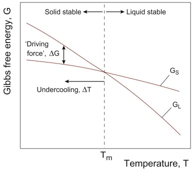
Figure 19.8 Schematic variation of free energy G with temperature for pure liquid (GL) and solid (GS). Above the melting point Tm, GL < GS and liquid is the equilibrium state; below Tm, solid is stable, and GS < GL. The driving force ΔG is the difference between the two curves when, for example, liquid is undercooled by an amount ΔT below its melting point, as shown.
It is straightforward to show how the driving force varies with the undercooling ΔT. Consider liquid and solid at the melting point Tm, where the free energies are equal:
Hence the changes in enthalpy and entropy between solid and liquid are related by

The enthalpy change ΔH (= HL – HS) may be familiar already as the ‘latent heat of melting’—the heat that must be applied to change solid to liquid at its melting point. The entropy increases in proportion, as in equation (19.3), giving no net change in free energy G.
Now if we undercool the liquid to a temperature T below the melting point, the driving force is given from equation (19.2) as
For modest undercooling, neither ΔH nor ΔS change much with temperature, so we can substitute from equation (19.3), giving
So to a first approximation the driving force for a phase change on cooling increases in proportion to the undercooling (or conversely the superheating on heating). Solid-state phase changes follow exactly the same principles, but with driving forces that turn out to be of the order of around one-third those for solidification. There is still ‘latent heat’ released at constant temperature when a solid crystal changes into another solid phase (or phases), but it is smaller. Similarly the entropy change associated with a change between two crystals is lower, as both still have a high degree of order.
As noted earlier, microstructures also evolve without the phases changing. An example is precipitate coarsening, in which a population of precipitates of various sizes evolves such that the average size increases. Small ones dissolve back into the surrounding matrix, and their atoms diffuse over and attach to the larger ones. We can still approach this using thermodynamics, considering free energy before and after the change. But in this case it is not a change of phase driving the process, but the energy associated with the interface between the precipitates and the surrounding matrix. This surface energy between two different crystals is associated with the atomic misfit between the phases across the boundary between them. It is analogous to the ‘surface tension’ that tries to pull water droplets to be spherical. The surface energy of the system is the surface energy per unit area, γ, times the total area of interface. Hence coarsening occurs because the total surface area falls if the precipitates form a smaller number of larger particles.
Other important examples in metals processing are recrystallisation and grain growth. Deformed metals are packed full of dislocations, with an associated energy per unit length (introduced as equation (6.9)). Recrystallisation wipes out the deformed grains, replacing them with new grains of much reduced dislocation density (see later)—the driving force is the change in stored dislocation energy. The grains may then grow, meaning boundaries migrate such that small grains disappear and the average grain size increases. Grain boundaries also have surface energy associated with the misfit in the lattice—larger grains means less area of boundary, and a reduction in system energy.
Returning now to the solidification example, equation (19.5) shows that the more we cool down, the more energy is available to drive solidification. We might therefore expect solidification (or any other phase change) to go faster and faster the more we cool a liquid below the equilibrium temperature. But this is not the case. To borrow a mathematical phrase, we might say that having thermodynamics on our side is a necessary condition, but it is not sufficient. It is also essential to have a kinetic mechanism by which the microstructural change takes place. Atoms are being asked to relocate, which in the vast majority of cases means they must diffuse (even if they only need to hop a fraction of the atomic spacing). This brings in a further dependence on temperature, and also (crucially) a dependence on the time available—both things that are strongly influenced by the manufacturing process (witness the bike frame example in Section 19.2).
The kinetics of diffusion were discussed in Chapter 13, principally in relation to creep of materials when used at elevated temperatures. Diffusion is at the heart of material processing too. Recall from Section 13.4 that there is a strong exponential temperature-dependence of the rate of diffusion, known as Arrenhius’ law:
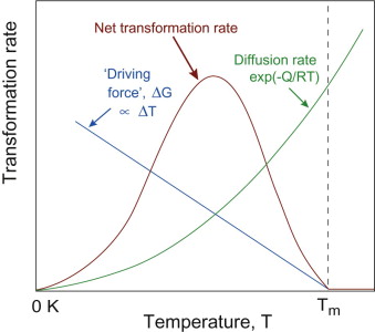
The rate of a phase transformation therefore depends on both the driving force and the diffusion rate. Their temperature-dependencies are in opposition—the more we cool, the higher the driving force but the lower the diffusion rate. How do they trade off? Figure 19.9 shows what happens. At low undercooling, diffusion is rapid but the driving force is small, falling to zero at the equilibrium temperature—the net transformation rate is low, limited by the driving force. At the other extreme (approaching zero Kelvin) the driving force is maximised, but diffusion is now so slow that nothing can happen. Somewhere in between, a maximum transformation rate is found where both thermodynamics and kinetics are favourable. This is an important and counter-intuitive outcome—diffusion-controlled changes go fastest at some particular undercooling, not when they are hottest.
Nucleation and growth
There is a further refinement we should know about in materials processing. When a liquid solidifies, solid first has to appear from somewhere, after which the interface between solid and liquid can migrate to enable atoms to switch from one phase to the other at the boundary. We call these two stages nucleation and growth (see Figure 19.10). Nucleation presents another subtlety of thermodynamics. At first glance, there is a driving force, so surely off it goes? But the first nuclei to form generate an interface that wasn’t there before (between the liquid and solid).
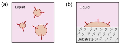
Figure 19.10 Nucleation and growth, illustrated for solidification. In (a) the solid nucleus forms spontaneously as a sphere within the liquid (homogeneous nucleation); in (b) the solid nucleus forms as a spherical cap on a solid substrate, such as the mould wall (heterogeneous nucleation).
It was noted earlier that interfaces between phases have an associated surface energy (due to the atomic mismatch). So some energy has to be provided to create this interface, and the source of this energy is the free energy of the transformation. But the energy released depends on the volume of the new phase formed, whereas the energy penalty at the interface depends on the area of its surface. For small particles of the new phase the surface area energy represents a significant barrier to transformation; for larger particles the volumetric energy release dominates. As a consequence of this trade-off there is a critical radius for nucleation. Only above this size do nuclei become stable and grow—smaller nuclei are unstable and melt back into the liquid.
The size of nuclei formed spontaneously is a statistical phenomenon, but it depends on the same factors as the growth rate (the driving force and the diffusion rate). The nucleation rate therefore follows the same form of temperature-dependence as shown in Figure 19.9 (although the temperatures at which maximum nucleation and growth rates occur do not coincide). But as both tend to zero at the equilibrium temperature and at zero Kelvin, the net transformation rate must still peak somewhere in between. This is why Figure 19.9 may be regarded as the temperature-dependence of the overall transformation rate.
The spontaneous formation of new phases, such as solid crystals within the bulk of a liquid, is strictly known as homogeneous nucleation. Figure 19.10 also shows an alternative way to start a transformation, with the new phase attaching itself to some other interface in the system, such as the surface of the mould holding the liquid. This is called heterogeneous nucleation. It turns out that the amount of undercooling needed for this route is significantly smaller than for homogeneous nucleation, so in practice heterogeneous behaviour dominates. Qualitatively we can see why. Figure 19.10 shows the same volume of new solid formed by both nucleation mechanisms. Three different surface energies are involved in the heterogeneous case (between liquid, solid and the additional material such as the mould), with various interfaces being created and eliminated. But the net effect is that the solid-liquid interface achieves a large radius (bigger than the critical radius) with far fewer atoms. The solid-liquid interface can then grow stably as if it is part of a much bigger nucleus, but with a much reduced surface energy penalty. Metals processing often exploits heterogeneous nucleation to influence the length scale of the new microstructure being formed (particularly grains). Examples are provided later.
Time-temperature-transformation (TTT) diagrams and the critical cooling rate
Foundry engineers worry about how long it takes for a casting to solidify, rather than the rate at which the solid-liquid interface is moving. But it is clear that these are directly related—inversely in fact, the faster the transformation rate, the sooner it will both start and finish. First we flip Figure 19.9 on its side, so that it shows temperature against rate of transformation (Figure 19.11); then we can infer the figure shown to the right, in which the time taken to reach a given fraction transformed is a minimum where the rate is a maximum, and the time tends to infinity for the temperatures at which the rate falls to zero. The characteristic shape of the curve leads to the name of ‘C-curve’ for these plots of diffusion-controlled phase transformations. A set of C-curves, as in the figure, depicts the onset and progress of a transformation to its completion. The net picture is called a time-temperature-transformation (TTT) diagram. For some heat treatments (notably steels) these are as central to processing as the phase diagram.
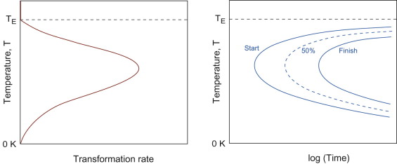
Figure 19.11 Temperature against the rate of transformation, and the corresponding form of temperature-time-transformation (TTT) diagram—maximum rate leads to minimum transformation time. ‘C-curves’ are shown for the start, 50% completion and finish of the transformation.
TTT diagrams are widely used to study diffusion-controlled transformation rates. The C-curve shape reflects the transformation rate as a function of temperature, assuming that we somehow cool rapidly from above the transformation temperature and hold isothermally at a fixed undercooling. This is fine in the laboratory with small samples, but real processing involves continuous cooling from above the transformation temperature to room temperature. In this scenario we reach for a variant set of curves called CCT diagrams (i.e. ‘continuous-cooling transformation’). Without going into details, the essential C-shape is retained in continuous cooling (though the curves are shifted to longer times and lower temperatures).
Figure 19.12 shows the temperature histories that are valid for each type of diagram. From this we should extract one core idea: in continuous cooling there is a critical cooling rate, that just avoids the onset of the diffusional transformation. If the cooling rate exceeds this value then (in general) the initial state at high temperature is retained, at a temperature when it is no longer the equilibrium state, but is unable to transform because the kinetics are much too sluggish. In thermodynamics terms this is a metastable state. Forcing components to cool at an accelerated rate is a common trick in heat treatment, to deliberately bypass equilibrium and achieve an alternative microstructure as a route to better properties than slow cooling.
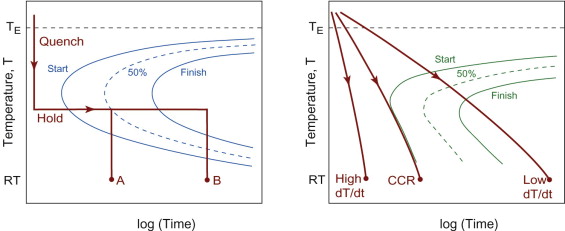
Figure 19.12 (a) A TTT diagram, interpreted for quench-and-hold isothermal treatments to room temperature (RT); at B the transformation is 100% complete, while at A a ‘split transformation’ has occurred, with only 50% transformed; (b) a CCT diagram, broadly the same shape, but for continuous cooling histories. The critical cooling rate (CCR) is the minimum rate that avoids the start of any diffusion-controlled transformations.
Guided Learning Unit 2: phase diagrams and phase transformations (Parts 5–8)
At this point, we recommend that you finish working through the Guided Learning Unit 2 (Parts 5–8). These sections illustrate the evolution of microstructure for a number of important processes (solidification and heat treatment), in relation to the relevant phase diagrams.
The rest of this chapter illustrates a range of manufacturing processes, and the microstructural evolution that takes place during processing. These case studies illustrate how control of composition and cooling history determine the microstructure in industrial processes, and thus how we can achieve the desired properties, if we follow the recipe correctly.
19.5 Metals processing
Metals—overview
It was clear in Chapter 18 that a favourable characteristic of metals is the diversity of manufacturing processes available to make and assemble components of complex shape. We now explore how, during processing, the underlying microstructure and thus properties are evolving. This includes both properties relevant to the process itself (for example, ductility for deep drawing a beer can) and the properties needed in service (for example, strength and toughness for automotive and aerospace alloys).
To illustrate the breadth of metals processing and property manipulation, we draw on examples from casting, deformation, heat treatment, joining and surface engineering. Steels (and other ferrous alloys) are the dominant engineering alloys, followed by aluminum alloys, so these feature in most of the examples. But similar principles apply to all the alloy systems, such as those based on Cu, Ti, Ni, Zn, Mg and so on. Most alloy systems offer both cast and wrought variants, and many are also processed as powder. Usually either cast or wrought alloys dominate an alloy class. This reflects subtle differences in the ease of deformation of the underlying crystal structures in different elements. For example, Zn, Mg and Ti have the ‘hexagonal close-packed (HCP)’ crystal structure (see Chapter 4). This is inherently less ductile than the FCC or BCC crystal structures found in Al, Fe and Cu—so Zn, Mg and Ti are mostly cast, with only limited deformation processing being conducted, and usually then done hot (when the ductility is better). Ductile Al, Fe and Cu are mostly wrought, but all come as casting alloys too.
Casting and wrought alloys in a given metal system tend to have quite different compositions. Good castability requires much higher levels of alloying additions than the relatively dilute wrought alloys (to lower the melting point). Casting leads to coarser microstructures and poorer strength and toughness than in wrought alloys (as illustrated for aluminum alloys in Chapter 8).
Solidification: metal casting
Casting is a relatively cheap shaping route, and is well suited to making complex 3-D shapes. It is used over a wide range of size, from large ship propellers to engine parts, machinery and sculptures, down to toys, household fittings and medical implants. Tweaking the chemistry of castings to improve their properties has been a bit of a black art for centuries. Nowadays it is possible to use sophisticated software tools to model everything from the choice of composition to the way to pour the metal into the mould in order to control the grain size and to minimise porosity and residual stress.
In casting, a liquid above its melting point is poured into a mould, where it cools by thermal conduction. New solid forms by nucleation, with crystals forming spontaneously in the melt, or on the walls of the mould, or on foreign particles in the melt itself (Figure 19.13(a)). The nuclei grow by diffusive attachment of atoms at the liquid–solid interface. Solidification is complete when crystals growing in opposing directions impinge on one another, forming grain boundaries—each original nucleus is the origin of a grain in the solid (Figure 19.13(b)). The grain size of the casting thus depends on the number of nuclei, since each one grows into a grain. Achieving a fine grain size, often important in achieving optimal properties, is assisted by controlling nucleation through the addition of inoculants—fine-scale solid particles that stimulate heterogeneous nucleation. An example is the addition of TiB2 to aluminum castings. At the other extreme, we sometimes wish to grow a single crystal, with no grain boundaries at all. An example is the casting of Ni superalloy turbine blades for jet engines. In this case it is a question of retaining just one nucleus, something that can be done by cooling the liquid slowly from one end so that the first nucleus to appear is made to grow along the entire length of the component. Examples of cast microstructures for different alloy compositions are illustrated in Guided Learning Unit 2.
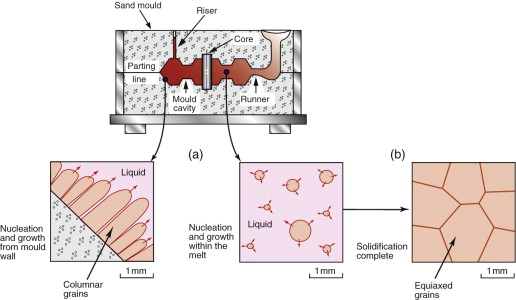
Figure 19.13 Solidification in metal casting: (a) nucleation and growth of solid crystals in the melt; (b) impingement of growing solid crystals forms the grains and grain boundaries.
The rates of nucleation and growth (and thus grain size) also depend on the imposed cooling history and this is governed by heat flow. This is a multi-parameter problem: it depends on the thermal properties of the metal and the mould, the contact between the two, the initial liquid temperature, the release of latent heat on solidification and the size and shape of the casting. Here is an example of the design–process–material coupling discussed in Chapter 18: the geometry of the design combines with the type of casting process (mould material, metal temperature, etc.) and the choice of alloy to dictate the cooling rate; and the microstructural response to that cooling rate (and thus properties) depends on the alloy chemistry.
A further complication in casting is that the liquid has a uniform concentration of solute but the solid does not. The solubility of impurities and solutes in the solid is less than that in the liquid, so they are rejected ahead of a growing crystal, enriching the remaining liquid. Concentration gradients build up in the solid grains with higher solute and impurity levels in the last part to solidify (i.e. the grain boundaries). This segregation is explained further in Guided Learning Unit 2. It can be a source of problems such as embrittlement or corrosion sensitivity at the boundaries. Castings therefore are often held at high temperature for prolonged periods (homogenisation) to enable some levelling out of the solute concentration gradients. In the case of impurity segregation, it is impractical and expensive to try and remove them from the melt. The trick is to render them harmless by giving them something else to react with, to form a solid compound distributed throughout the casting. For example, manganese is added to carbon steels in order to wrap up the impurity sulfur as harmless MnS, rather than letting it concentrate at the grain boundaries as brittle FeS.
The difference in solubility between liquid and solid is also a problem with respect to gaseous impurities dissolved in the melt. On solidification, most of the dissolved gas is rejected into the remaining liquid, but must eventually be released as a separate phase—in this case as trapped bubbles of gas. As a result, castings inevitably contain some porosity. Good casting practice traps these bubbles as microporosity throughout, rather than sweeping all the gas into a big cavity in the middle of the component. Better still, but more expensive, the liquid is ‘out-gassed’ under vacuum just before it is poured. In the case of steel-making, high levels of dissolved gas are a direct consequence of previous processing of the melt—the carbon content is reduced to the required level by injecting oxygen into high carbon molten iron, but this leaves oxygen and carbon monoxide/dioxide in solution. To deal with this, reactive elements such as aluminum may be added to the melt prior to casting. These react with oxygen in solution to form solid oxides, which are again trapped as harmless particles in the casting—a trick known as ‘killing’ the steel. It is another example of how a small alloying addition is used to fix a problem due to the presence of a trace impurity.
Deformation processing of metals
Solid-state deformation processes (rolling, forging, extrusion, drawing) exploit the plastic response of metals, in particular their ductility, that is, their ability to remain intact without damage when subjected to large strains and shape changes. Most processes are compressive rather than tensile, to avoid the problem of necking in tension. And in many cases forming is conducted hot, to exploit the reduced yield stress—alloys at temperature can effectively be forced to creep at high strain-rates. Wrought metal products (i.e. shaped by deformation) are as ubiquitous as castings: beams, columns and tubes for buildings and offshore structures; bodies, panels and engine parts for every type of vehicle; machinery, tools, pipework, wire, food and drink containers—the list goes on. Deformation not only makes the required shape, it also drives the internal changes in microstructure. The component temperature, strain-rate and strain control both the flow stress during shaping, but also the material internal state during and after forming.
First, the temperature determines the phases present (see Guided Learning Unit 2, and Figures 19.6 and 19.7). This affects the material strength during forming, but has implications for what happens during cooling afterward. For example, hot rolling of carbon steels takes place in the austenite field, at temperatures of 900 °C or more (Figure 19.7). On cooling, rolled carbon steels will typically follow equilibrium, leading to a mixture of grains of ferrite and pearlite (the latter being a two-phase mixture of iron carbide and ferrite). The mechanism of this transformation is described in Guided Learning Unit 2. But the grain size and proportions of ferrite and pearlite (and hence properties) vary in fine detail, depending on the steel composition and the cooling rate. And the thermal history will depend on the initial temperature, the size and shape of the component and how the product is handled after shaping (e.g. thin strip is coiled and as a result remains hot for longer).
The second generic microstructural issue in deformation processing is the development of grain size. We have seen how casting leads to the initial solid grain size. Perhaps surprisingly, the grain size can be manipulated further in the solid-state. In the first instance, when the component changes shape, the grains inside follow suit to accommodate the overall strain. Figure 19.14(a) shows schematically how rolling ‘pancakes’ the grains. This can give a bit of useful longitudinal strengthening, rather like a fibre composite. More significantly the microstructure within the grains is modified: work hardening occurs, increasing the dislocation density. If this is the final shaping step, this is exploited to strengthen the final product, for example, deep drawing the walls of an aluminum beverage can, or drawing a copper wire. For earlier forming stages however, work hardening is a problem as it pushes up the forming loads, and limits the ductility. It is therefore necessary to anneal the metal (soften with heat), and this heat treatment offers the opportunity to control the grain structure too.
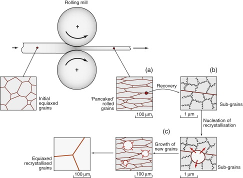
Figure 19.14 Grain structure evolution in the solid state by deformation and annealing: (a) grains follow the shape change in the component; (b) the recovery mechanism: dislocations re-arrange as subgrains (note the magnified scale); (c) the recrystallisation mechanism: new grains form by migration of boundaries from a few subgrain nuclei, replacing the deformed microstructure.
Annealing involves recovery and recrystallisation, which are solid-state changes in the dislocation and grain structure at elevated temperature. This may require a separate heat treatment after forming, but they can also take place concurrently during hot deformation. In recovery, dislocations interact and rearrange into organised patterns forming subgrains, which are like tiny grains within grains (see Figure 19.14(b)). More prolonged heating leads to recrystallisation, shown in Figure 19.14(c). Grain boundaries migrate by atoms hopping from old to new grains at the boundary between the two. This sweeps up and eliminates most of the stored dislocations, removing the work hardening completely. This lowers the yield stress, making it easier to work the material to shape—something blacksmiths have known for centuries, though they had no idea of the microstructural changes.
As noted earlier, recrystallisation has a driving force (the stored dislocation energy) and a kinetic mechanism (boundary migration), though it is not a phase transformation. In common with solidification however, the resulting grain size depends on the number of nuclei, here the number of sub-grains that exceed a critical size and migrate during recrystallisation. The metallurgy of recrystallisation is a complex matter—it depends on the initial grain size, the deformation conditions (temperature, strain and strain-rate), and the annealing temperature. Furthermore, all the nucleation is heterogeneous—either on grain boundaries (as shown in Figure 19.14(c)), or from small hard particles of intermetallic phases within the grains (so-called ‘particle-stimulated nucleation’). This population of particles is itself a consequence of the alloy chemistry, and the upstream processing stages of casting and homogenisation when the particles are formed.
The scope for manipulating the grain structure during forming is therefore a major distinction between the cast and wrought alloys. The grain sizes in wrought alloys are much smaller (typically 10–100 µm). But it is one of the most coupled, multi-variable problems to control, dependent on alloy composition, deformation rate, process temperatures and component geometry and strain. It is therefore difficult to get a uniform grain size in a formed part, as the strain, strain-rate and temperature vary with location.
As if this wasn’t enough, there is another important side-effect of deformation and annealing: the concept of crystal texture. The crystal planes in a casting are random—each nucleus forms in isolation within a melt. Not only does deformation ‘pancake’ the grains, it also tends to align the crystallographic planes with respect to the axes of the deformation. Perhaps unexpectedly, recrystallisation does not restore randomness—there remains a statistical distribution of orientations. This doesn’t sound very important, but it is significant in working with sheet metal, since textured metals have yield properties that are anisotropic (i.e. different in different directions). This can be a problem if you want to make something smooth and circular out of a sheet, like a beverage container.
Heat treatment of metals
Wrought metal products, and some castings and powder processed parts, are often subjected to heat treatment. This serves various purposes. Annealing to soften an alloy before further forming is one. Normalising is another—slow cooling from high temperature as the final step in making a component, the object being to minimise the final residual stress, and to produce a microstructure of lower strength but high toughness. Many alloys also undergo final heat treatments to enhance strength by precipitation hardening. Maximising strength without loss of toughness is essential for many heavy duty applications of steels (e.g. gears, cranks, cutting tools). And it is essential in combination with low density in the aluminum alloys used widely for aircraft structures.
In a typical heat treatment, the shaped component is heated to high temperature, cooled at a controlled rate and (usually) reheated to an intermediate temperature. This exploits the solid-state phase changes that occur with temperature, the use of a quench to avoid transformations that are ineffective for hardening and finally low temperature precipitation for maximum strength. Figure 19.15 illustrates a common sequence:
- Solutionize at elevated temperature, to form a solid solution.
- Quench to room temperature at a cooling rate dT/dt above the critical cooling rate (defined in Figure 19.12); this retains the high-temperature solid solution state at room temperature, avoiding the diffusion-controlled transformations to equilibrium phases.
- Precipitate fine-scale phases in the subsequent reheat.
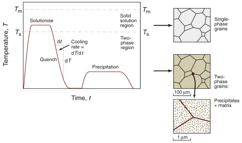
Figure 19.15 Schematic thermal profile for heat treatments that produce precipitation hardening, illustrating microstructural changes being induced: a solid solution at high temperature, and precipitation of hardening particles (shown at an enlarged scale) at a lower temperature.
Precipitation hardening is a generic mechanism in many alloy systems, but two heat treatments of this type are particularly prevalent: the ‘quench and temper’ of steels, and ‘age hardening’ of aluminum alloys. These are discussed in more detail in Guided Learning Unit 2. Although both follow the general picture illustrated in Figure 19.15, there are subtle microstructural details in each case.
First consider age hardenable Al alloys. On quenching the supersaturated solid solution is found to have modest strength. Then during ageing the yield strength rises to a peak, significantly harder than that produced by coarse equilibrium precipitates on slow cooling. But this is not only because of the fine scale of the precipitates formed—age hardening exploits the formation of metastable phases rather than the equilibrium phases. The effectiveness of age hardening for enhancing strength in aluminum alloys was illustrated in Chapter 8 on a fracture toughness–strength property chart (Figure 8.15). Below we trace the responses of carbon steels on the same property chart.
Consider now the quench and temper treatment for carbon steels, which proceeds as follows. The first stage is to solutionise in the FCC austenite field (austenitisation), dispersing the carbon into solid solution. Quenching to room temperature traps the carbon in supersaturated solution. But there is also the FCC to BCC phase change in iron to be accommodated. In spite of the quench this still takes place, by an unusual diffusionless mechanism (see Guided Learning Unit 2). The result is a metastable phase called martensite. The supersaturation of carbon causes severe distortion of the BCC iron lattice, giving martensite a high yield strength but very low fracture toughness. In this state the component is too brittle to place in service, and is susceptible to cracking during the quench due to induced thermal stresses. It is essential to restore the toughness, and this is achieved by tempering at an intermediate temperature. This leads to precipitation of the equilibrium phase, iron carbide. The yield strength falls as toughness is restored, but the final yield strength is substantially higher than that of the ferrite-pearlite microstructure formed on slow cooling.
The effectiveness of quenching and tempering may be illustrated via a fracture toughness–strength property chart, shown in Figure 19.16. The figure is annotated with selected micrographs. First the effect of carbon content on the properties in the normalised condition can be seen: from 0 to 0.8 wt% carbon the strength increases steadily as the proportion of pearlite to ferrite increases. Then taking a medium carbon steel (0.4 wt% C) as an example, we see how quenching produces the unusual microstructure and properties of martensite, en route to the final tempered condition (which can be fine tuned by choice of temper temperature, as shown in the Figure). Note that the precipitation during tempering is too fine-scale to be resolved in an optical micrograph—the appearance remains similar to martensite. Quenching and tempering are further enhanced by making alloy steels—carbon steels with modest alloying additions—as discussed in the case studies below.
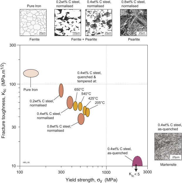
Figure 19.16 Fracture toughness–yield strength property chart for plain carbon steels, showing the effect of carbon content in the normalised condition, and the effect of quenching and tempering for medium carbon steel. Selected micrographs show the corresponding microstructures.
(Images courtesy: ASM Micrograph Center, ASM International, 2005)
Joining processes
Thermal welding of metals involves heating and cooling. This may cause phase transformations: (1) in the ‘weld metal’, which is like a localised miniature casting, melting and resolidification occur; (2) in all the heated regions of the weld, solid-solid phase changes occur on cooling, as in a heat treatment process. The solid region surrounding the melt pool where microstructural changes occur is referred to as the ‘heat-affected zone’. The evolution of microstructure and the consequent property changes in the HAZ depend on the thermal cycles imposed. Once again the thermal history couples the material, the way the process is operated (e.g. power input) and design details such as joint thickness. Thermal welding can have major consequences for joint performance—depending on the alloy and the welding process, the material may be softened, or embrittled or lose its corrosion resistance.
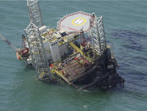
Figure 19.17 illustrates the contrasting responses to welding that are commonly observed in low-carbon and low-alloy steels, and heat-treatable aluminum alloys. Hardness profiles are the simplest first indicator of property changes across a welded joint. Low carbon steels are considered to be weldable, as on cooling the material reverts to ferrite and pearlite—the weld and HAZ have similar hardness to the original material. Low alloy steels form martensite more easily, as the critical cooling rate is lower, increasing the risk of weld embrittlement (the high hardness of martensite being a characteristic indicator). Oil rigs and bridges have collapsed without warning as a result of this behaviour, usually because the welding process was conducted incorrectly, leading to cooling rates that are too high. Heat-treatable aluminum alloys are age hardened to their peak strength—on welding there is only one way for the hardness to go, and that is down. Over-ageing due to the weld thermal cycle can lead to a permanent loss of 50% or more of the strength. In more weldable Al alloys, the metastable precipitates dissolve instead, enabling some subsequent recovery of strength by room temperature (‘natural’) ageing.
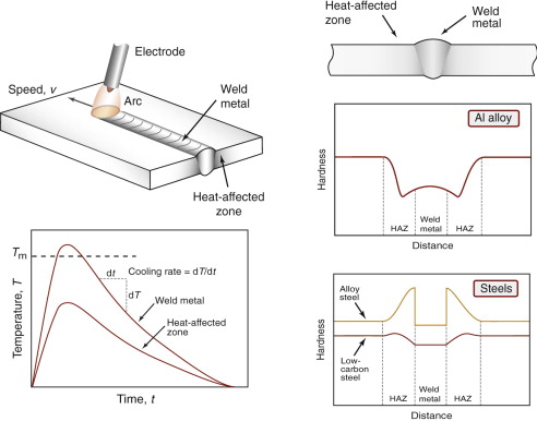
Figure 19.17 A weld cross-section with corresponding thermal histories in the weld metal and heat-affected zone. To the right are typical hardness profiles induced across welds in heat-treatable aluminum alloys, low carbon steel and low alloy steel.
Welding metallurgy is therefore a big field of study—welds are often the ‘Achilles heel’ in design, being the critical locations that determine failure and allowable stresses. This may be because the material properties are damaged in some way at the joint (as shown earlier), or it may also be due to other side-effects of the process (residual stresses, or stress concentrations or crevices, potentially causing fatigue and corrosion problems). Some mechanical joining processes (e.g. friction welding) also lead to local changes in microstructure and properties, by deformation as well as heat. Adhesive technologies have the advantage that they don’t impose, deform or heat the components being joined, leaving the microstructure and properties intact. But they are not trouble free—they still concentrate stress and contain defects, requiring good design and process control.
Surface engineering
Surface treatments exploit many different mechanisms and processes to change the surface microstructure and properties. Some simply add a new coating material, with its own microstructure and properties, leaving the substrate unchanged—the only problem is then making sure they stick. Others induce near-surface phase transformations by local heating and cooling—transformation hardening. Figure 19.18 shows an example—laser hardening of steels. The laser acts as an intense heat source traversing the surface, inducing a rapid thermal cycle in a thin surface layer. Heating depths of order 1 mm into the austenite field is readily achieved, with conduction into the cold material underneath providing the quench needed to form martensite. The high hardness of martensite gives excellent wear resistance, and the brittleness is not a problem when it is confined to a thin layer on a tough substrate.
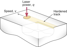
Figure 19.18 Laser hardening: a surface treatment process that modifies microstructure. The traversing laser beam induces a rapid thermal cycle, causing phase changes on both heating and cooling. The track below the path of the laser has a different final microstructure of high hardness.
Direct diffusion of atoms into the surface is also feasible, but only for interstitial solute atoms at high temperature for diffusion to occur over a distance of any significance. Chapter 13 revealed that, even near the melting point, there is a physical limit to diffusion distances ![]() of around 0.2 mm for a 1 hour hold, which is sufficient for surface treatments (and also for bulk processing on a very small scale, as in semiconductor devices). This mechanism is used to increase the carbon content (and thus hardness) of steels—the surface treatment known as carburising. Even better is a hybrid surface treatment: first carburise, and then transformation harden too, giving very hard high carbon martensite.
of around 0.2 mm for a 1 hour hold, which is sufficient for surface treatments (and also for bulk processing on a very small scale, as in semiconductor devices). This mechanism is used to increase the carbon content (and thus hardness) of steels—the surface treatment known as carburising. Even better is a hybrid surface treatment: first carburise, and then transformation harden too, giving very hard high carbon martensite.
Case studies: ferrous alloys
For structural and mechanical applications, steels and other alloys based on iron dominate. They are intrinsically stiff, strong and tough and mostly low cost. High density is a drawback for transport applications, allowing competition from light alloys, wood and composites. Figure 19.19 illustrates the diversity of applications for ferrous alloys. These reflect the many classes of alloy—different chemistries combined with different process histories. Examining each in turn highlights the key material property, composition and processing factors at work.
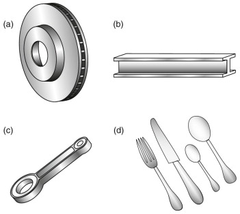
Figure 19.19 A selection of products made from alloys based on iron: (a) cast iron: brake disk; (b) low carbon steel: I-beam; (c) low alloy steel: connecting rod; (d) stainless steel: cutlery.
Cast iron: brake disk
Brake disks (Figure 19.19(a)) use sliding friction on the brake pads to decelerate a moving vehicle, generating a lot of heat in the process (Chapter 11). The key material properties are therefore hardness (strength) for wear resistance, good toughness and a high maximum service temperature. Low weight would be nice for a rotating part in a vehicle, but this is secondary. All ferrous alloys fit the bill—so why cast iron? This is because casting is the cheapest way to make the moderately complicated shape of the disk, and the as-cast microstructure usually does not require further heat treatment to provide the hardness required. The carbon content of cast irons is typically 2–4% (by weight) giving a lot of iron carbide, the hard compound in ferrous alloys giving excellent precipitation hardening. Cast irons can also be transformation hardened at the surface to enhance their wear resistance (e.g. by laser hardening).
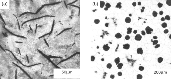
Cast irons illustrate another way in which minor alloying additions are used to make significant microstructural modifications, with consequent property changes. Figure 19.20(a) shows the microstructure of gray cast iron, containing thin flakes of graphite as one of the phases present. The surrounding matrix is a mixture of ferrite and iron carbide. In this form cast iron has excellent machinability, that is, it can be machined quickly with minimal or no lubricant, an example of a property that is important during processing, rather than in service. The graphite flakes are brittle and crack-like, making it easy for chips to break off during machining. But in service this brittleness may be a problem. Cast iron microstructures can be toughened using an alloying trick called poisoning. The addition of a small amount of cerium or magnesium, sometimes with a prolonged annealing treatment, has the effect of radically changing the morphology of graphite in iron, so that the graphite spherodises to minimise the surface area of interface. By avoiding the crack-like flake form of graphite, the fracture toughness and failure strength of the cast iron are enhanced (illustrated later). The surrounding matrix may be ferritic or pearlitic, depending on alloy and the cooling history. Figure 19.20(b) shows such a ‘nodular’ cast iron containing spheroidal graphite, with in this case a surrounding matrix of ferrite. Note that the carbon content in both figures is the same. This poisoning technique is also used to enhance toughness in Al-Si casting alloys—small sodium additions lead to the brittle Si forming fine-scale rounded clumps, rather than the plates and needles characteristic of solidification of eutectic compositions (see Guided Learning Unit 2).
Plain carbon steel: I-beams, cars and cans
If we had to single out one universally dominant material, we might well choose mild steel—iron containing 0.1–0.2% carbon. Almost all structural sections (Figure 19.19(b)), automotive alloys and steel packaging (beer and food cans) are made of mild steel (or a variant enhanced with a few other alloying additions). All of these applications are wrought—the alloy is deformed extensively to shape. The microstructure consists of ferrite and a small amount of pearlite. This provides the excellent ductility needed both for processing and in service. The fracture toughness is high, and combined with the inherent strength of iron, which may be increased by deformation processing (work hardening). Ductility, toughness and decent strength are vital in a structural material—we would rather a bridge sagged a little rather than broke in two, and in a car crash our lives depend on the energy absorption of the front of the vehicle.
Alloy steels and heat treatment: cranks, tools and gears
The moving and contacting parts of machinery are subjected to very demanding conditions—high bulk stresses to transmit loads in bending and torsion (as in a crank or a drive shaft), high contact stresses where they slide or roll over one another (as in gears) and often reciprocating loads promoting fatigue failure (as in connecting rods, Figure 19.19(c)). Strength with good toughness is everything. Plain carbon steels up to 0.8 wt% C give effective precipitation hardening, particularly when quenched and tempered (Figure 19.16). But the density of iron is a problem. Make the steel stronger, and use less of it, and we can save weight. This is particularly true for fast-moving parts in engines, since the support structure can also be made lighter if the inertial loading is reduced (so-called ‘secondary weight savings’). By now the solution should not be a surprise: yet more alloying, and more processing.
A bewildering list of additions to carbon steel can be used to improve the strength—Mn, Ni, Cr, V, Mo and W are just the most important! Some contribute directly to the strength, giving a solid solution contribution (e.g. high-alloy tool steels, with up to 20% tungsten). More subtle though is the way quite modest additions (<5% in low-alloy steels) affect the alloy’s response to the quench and temper heat treatment (discussed earlier for plain carbon steels). The problem with quenching plain carbon steels is that the critical cooling rate is high. As a result, only thin sections can be quenched to form martensite—the cooling rate within the component being physically limited by heat flow, governed by the component thickness and the inherently low thermal conductivity of steel (compared to other metals).
Alloying solves the problem by slowing down the diffusional transformations to ferrite and iron carbide, shifting the C-curves of Figure 19.12 to much longer times. This enables slower quench rates to achieve the target martensitic microstructure. Hence bigger components can be quenched to this supersaturated state, and thus tempered. The technical term for the ability of a steel to form martensite is hardenability—the higher the hardenability, the lower the critical cooling rate, or the larger the component that will form 100% martensite. In high alloy steels, such as those used for cutting tools, the effect is so pronounced that cooling in air is sufficient to form martensite. An additional benefit of using alloy steels is that a bit of additional precipitation strength comes from the formation of alloy carbides (rather than iron carbide). Compounds such as tungsten carbide survive to higher temperatures than iron carbide without dissolving back into the surrounding iron—a useful source of high-temperature precipitation strength (e.g. for cutting tools).
So in its full complexity, heat treatment of steels presents another example in which the resulting properties depend on coupling between material, process and design detail—alloy composition determines the hardenability, and the quenching process and component size determine the cooling rate, and hence the microstructural outcome.
Stainless steel: cutlery
The city of Sheffield in England made its name on stainless steel cutlery (Figure 19.19(d)), and still manufactures steel (of all types) on a major scale. The addition of substantial amounts of chromium (up to 20% by weight) imparts excellent corrosion resistance to iron, avoiding one of its more obvious failings: rust. It works because the chromium reacts more strongly with the surrounding oxygen, protecting the iron from attack (Chapter 17). Nickel is also usually added for other reasons—one being the preservation of the material’s toughness at the very low cryogenic temperatures needed for the stainless steel pressure vessels used to store liquefied gasses. Another is that both chromium and nickel provide solid solution hardening—this and work hardening (during rolling and forging) being the usual routes to strength in stainless steels, though some Fe-Cr-C alloys are also heat treated for precipitation strength.
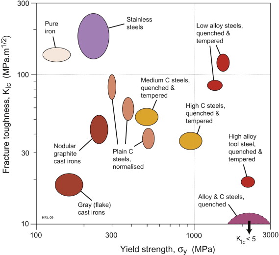
Ferrous alloys: summary
We have seen that in all of these applications, strength and toughness dominate the property profile. The variation of these properties for plain carbon steels was illustrated in Figure 19.16. In summary, we can map all classes of ferrous alloys on this chart. Figure 19.21 assembles the data for a selection of alloys from the classes discussed in the case studies discussed earlier. This paints a remarkable picture. Starting with soft, tough pure iron (top left), we can manipulate it, by changing composition and process history, to produce more or less any combination of strength and toughness we like—increasing the strength by a factor of 20 or more. Every final material (with the exception of as-quenched martensite) is above the typical fracture toughness threshold (<15 MPa.m1/2) for structural or mechanical application. Cast irons primarily offer low cost and lower pouring temperatures than pure iron, for a modest increase in strength, but note the effectiveness of poisoning in restoring toughness by forming nodular rather than flake graphite (Figure 19.20). The normalised condition is standard for structural use, unless the corrosion resistance of stainless steels is required. The chart shows the benefit of quench-and-temper treatments in raising the strength without damaging the toughness, particularly in alloy steels. This figure explains why ferrous alloys are so important—no other material is so versatile, with literally hundreds of different steels and ferrous alloys available commercially.
19.6 Non-metals processing
Ceramics and glasses
Ceramics and glasses are somewhat niche materials. Ceramic applications exploited their high hardness (cutting and grinding tools), high-temperature resistance (furnace liners) and high electrical resistivity (spark plugs, electronics, overhead power line insulators). Glasses are exploited mainly for optical properties, both in sheet and fibre form, and for containers such as bottles. But as brittle materials they have a problem. No matter what other advantages they have, they are susceptible to fracture, which may be traced back in many cases to the inherent defects built in during processing. Defect control is therefore a key factor in ceramic and glass processing for mechanical applications. The microcracks in ceramics largely reflect the size of powders used in the first place, but good-quality processing is then needed to avoid porosity. This is surprisingly difficult to achieve, even in simple shapes. Loose powders contract by a factor of 2 or more when they are pressed and sintered together. Achieving uniform contraction of this magnitude is not easy, since different regions of the product densify first and then constrain the further compaction of the remainder.
Glasses are easier to handle as they are melt processed. Nonetheless, great care is taken over achieving a smooth finish—plate glass is produced mostly by flotation on a bath of molten tin. Ceramics and glasses are also very susceptible to thermal stresses during cooling. Being processed at high temperature, but inherently stiff and strong, stresses are not easily relieved by creep during cooling. In one instance, however, thermal stresses are exploited to good effect. Glass can be made more fracture resistant by deliberately generating a residual stress profile through-thickness, by rapid cooling of the surfaces. This leads to beneficial compression at the surfaces and tension within—the surface being the likely location of the scratches and microcracks that cause fracture under tensile load.
Ceramic compositions tend to be largely discrete, each being a specific compound (alumina, silicon carbide, etc.). Some ceramic-metal composites are produced, such as tungsten carbide and cobalt, to make a hard, tough material for dies and cutting tools. In contrast, glass compositions can be tuned continuously over a wide range to achieve particular combinations of color and other optical properties (e.g. the graded compositions used in optical fibres). The adaptable spread of optical properties was evident in the property charts of Chapter 15. This is largely a matter of tweaking the chemistry rather than the process. More recent developments with glass processing are associated with coating technology, for scratch and chip resistance (in windscreens), or for self-cleaning and high reflectivity in high-rise buildings.
Powder processing
Ceramics, and also many metals, can be shaped by filling a mould with loose powder and compacting it. The main microstructural evolution is the shrinkage of porosity during compaction, with each particle becoming a final grain (Figure 19.22). Powder compaction mechanisms are closely related to diffusional flow and creep (Chapter 13). In purely thermal compaction (sintering), atoms diffuse along the particle boundaries to fill in the pores. Compaction is accelerated by imposing external pressure as well as temperature—‘hot isostatic pressing’ (or HIPing)—giving particle deformation by creep.
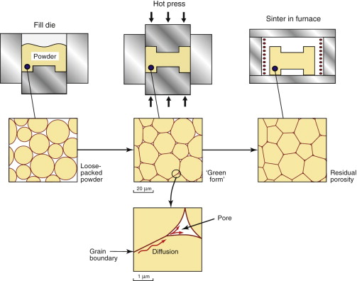
Polymers and elastomers
Polymers are versatile materials in many respects—easy to mould into complex shapes at low cost, easy to join together by snap fitting and easy to colour. Bulk polymers provide a spread of Young’s modulus, strength and fracture toughness, all relatively low. Polymer chemistry, and the use of additives and fillers, gives freedom to adapt the bulk properties, though the ability to make large changes in strength is more limited than for metals. But in contrast, polymers do offer scope for changing elastic properties, which metals do not. Polymers find widest application in packaging, and for diverse household and workplace applications (computer and phone casings, toys, pens, kitchen appliances and containers and so on). Design of these products mostly leads to only modest mechanical performance, but low cost and aesthetics dominate.
Chapter 4 introduced the structure of polymers, and how chemistry is used to produce the thousands of variants available today. Long-chain molecules are produced by polymerisation of a basic monomer unit of carbon, bonded with hydrogen, chlorine, oxygen and so on. Each monomer has a discrete chemistry—C2H4 makes polyethylene, for example. Unlike metal (and non-metal) atoms, monomers do not readily combine with one another. Only selected combinations will polymerise together, to make copolymers (with two monomers), terpolymers (with three) and so on. For example, ABS is a terpolymer, combining monomers of acrylonitrile, butadiene and styrene (hence the name). Blending polymers extends the range further, giving a mixture of more than one type of chain molecule—for example, ABS–PVC. And the molecular architecture itself can be manipulated. As described in Chapter 4, thermosets and elastomers are cross-linked, and some thermoplastics will partially crystallise. Furthermore, bulk polymers usually contain additives and fillers, for all sorts of reasons—for example, glass or ceramic particles or fibres (for stiffness, strength or colour), flame retardants, plasticisers or UV protection.
Polymer moulding
Most of the microstructural variety in polymers has only a modest impact on processing—most processes work with most polymers. Thermoplastics are moulded as viscous liquids. Additives change the viscosity, so the ease of moulding will be influenced by the volume fraction of filler. Injection moulding and extrusion dominate. Polymers mostly prefer to form an amorphous structure, but in some thermoplastics partial crystallinity may develop, the extent depending on the cooling rate. All polymers shrink as the mould cools from the moulding temperature to room temperature, because of both thermal contraction and the loss of free volume caused by crystallisation. Allowance must be made for this when the mould is designed. Fusion welding works only for non-cross-linked thermoplastics, which can be remelted.
Processing can play a significant role in determining the final molecular arrangement, and thus properties, if the molecules are first aligned mechanically by the flow induced during the shaping process, and cooling is then rapid enough to freeze in the alignment. Figure 19.23 shows the blow moulding of a drinks bottle, from a preform closed tube called a parison. In some variants the parison is stretched longitudinally with an internal rod prior to blow moulding. The stretching process of blow moulding aligns the molecules in the bottle wall, enhancing stiffness and strength. The degree of stretch is even customised to give greater enhancement in the circumferential direction, which carries the greater tensile stress under pressure.
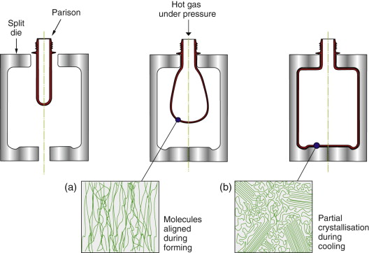
Polymer fibres
The most dramatic impact of processing on polymer properties is in making fibres. These are drawn from the melt, or for even better results, cold drawn. Now the molecular alignment is much more marked, so that the fibre properties exploit the covalent bonding along the chain. We can illustrate the resulting strength and stiffness on a property chart. To emphasise the lightweight performance with respect to other materials, Figure 19.24 shows the specific strength σy/ρ and specific stiffness E/ρ. Bulk polymers, in spite of all the chemical trickery, span only about a decade in strength and stiffness, and are outperformed by metals, particularly on specific stiffness. Standard polymer fibres of nylon or polyester are stiffer and over 10 times stronger than the bulk polymer. They quickly overtake most natural fibres, such as cotton and hemp, but not silk, which is a particularly good natural fibre. However, aramid fibres (such as Kevlar), and special grades of polyethylene fibres, are up to 100 times stiffer and stronger than bulk polymer, with specific properties close or superior to carbon and glass fibres.
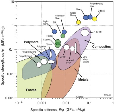
Figure 19.24 Specific strength–specific modulus property chart. Bulk polymers are stiffened and strengthened by drawing into fibres, competing with natural, carbon and glass fibres. Most products use the fibres in a composite, such as CFRP, or woven into a fabric.
Fibre properties are all very impressive—the problem though is getting the fibres into a form that is useful to the engineer. One option is composites—aramid fibres are used in the same way as carbon and glass fibres, in a matrix of epoxy resin. As discussed in earlier chapters, the resulting composites shown in Figure 19.24 lie between those of the matrix and fibre, where they compete strongly with the best of the metals, such as low-alloy steels. Alternatively, we use polymer fibres in exactly the way that natural fibres have been used for millennia: twisted, tangled or woven to make rope, cables, fabrics and textiles. Fibre-based materials are a whole discipline of materials engineering in themselves, with many important applications. The geometric structure of ropes and textiles is essential to the way they work—it is this that gives them flexibility in bending, combined with enormous stiffness and strength in tension. The drape of clothing exploits the differences in stiffness parallel to and at 45 degree to the weave (the ‘bias’). Ropes can be stretched, coiled and knotted elastically due to their twisted and woven architecture. The loss of alignment of the fibres in making a rope or weave does mean that their load-carrying capacity is never quite as good as that of the fibres themselves in their pristine form. Nonetheless it is clear from the property chart that cables based on the best polyethylene fibres, for example, can potentially compete with conventional steel cabling.
19.7 Making hybrid materials
Hybrids were defined in Chapter 2 as a combination of materials from different classes, one of which could just be air (as in foams). Making a hybrid is often a processing challenge, so we conclude the discussion of processing for properties with some examples. First we might ask: why bother with hybrids at all? The answer is simple: hybrids can occupy spaces on property charts not occupied by monolithic materials. Sometimes design requirements can be in direct conflict, with no single material able to provide the property profile needed—for example, high strength (for which alloys are best) and high electrical conduction (for which pure metals are best). Hybrids allow innovative design solutions and improvements in performance, exploiting the individual properties of the component materials. Hybrids take a variety of forms—a simple classification is illustrated in Figure 19.25. Composites are the most straightforward—particles or fibres of one material embedded in another. Next are sandwich structures—skins of high-performance material on a lower grade core. Lattices (random or regular) include foams and other highly porous materials, and segmented materials are made of interlocking strands or layers of materials—ropes and cables are often hybrids of several types of material.
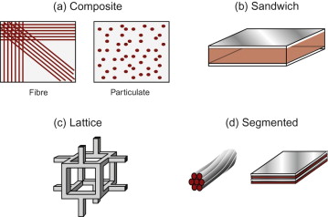
Figure 19.25 Classes of hybrid materials: (a) fibre and particulate composites; (b) sandwich panels; (c) lattice structures, such as foams; (d) segmented materials, such as ropes and laminates.
This classification is not 100% robust, since the boundaries get a bit fuzzy at the edges. For example, modern ‘nanocomposites’ are made by mixing nanometer-scale particulates into a molten metal and casting it—by Figure 19.25 this is a hybrid. However, heat treatment of steels produces an iron matrix with a fine dispersion of carbides—essentially the same microstructure, also produced for strength, yet we classify this as a metallic alloy. And at the other end of the scale, designing with a sandwich ‘material’ merges into designing a sandwich ‘structure’ (a ski, an aircraft floor panel or an industrial door). Essentially, we might define hybrids as structured materials whose component materials are routinely available in bulk and used in their own right, with the bulk materials and the hybrid having definable material properties. In spite of some non-uniqueness in this definition, hybrid materials can all be thought of as some combination of component (bulk) materials plus configuration and scale. Configuration defines the proportions, geometric integration and shape of the components; scale defines the length scale on which they are mixed. The length scales of hybrids are mostly relatively coarse—fibres of order 1–10 µm, and the layers of laminates and sandwich panels of order 0.1–10 mm. Bulk material microstructures span everything from the atomic scale (nanometers) up to the micron scale (see Figures 19.2–19.4). However, since hybrids combine the properties of the component materials, their properties reflect microstructure all the way from atomic to product scale.
Making foams
Foams extend the range of stiffness, strength and density axes of the property charts downward by several orders of magnitude. Some foams are made by trapping bubbles in a melt and solidifying the froth as a slab. Others are made by mixing in chemicals that react to form a gas, injecting it into a cavity and allowing it to inflate in situ as the gas bubbles are formed internally. The mechanical properties of an ideal foam depend systematically on the relative density (the fraction of solid), as shown in Chapter 4 for Young’s modulus. In practice it is found that the properties are also sensitive to the variability in pore size. It is important in processing to control the size of the largest pores, which initiate failure. Metal foams and rigid polymer foams can be made to shape and then cut and assembled into other structured materials (often as the cores of sandwich materials themselves).
Making composites
Most polymers are in fact particulate composites—bulk polymer melts to which filler powders have been added before moulding to shape. This is a hybrid that we opt to classify as a polymer variant—largely because the scale of the additives is very fine, almost at the scale of the polymer’s own molecular microstructure. Metal–matrix composites, on the other hand, are regarded as distinct hybrids—SiC particles in aluminum alloys, for example—but they too are processed in exactly the same way as the matrix aluminum alloy. Long fibre-reinforced polymer composites—CFRP, GFRP and Kevlar (aramid FRP)—require dedicated manufacturing techniques. Their potential performance in lightweight design has been clearly illustrated in earlier chapters, but can the ideal properties be achieved routinely in practice? The answer depends on the complexity of the component geometry and the impact of joining. Composites are straightforward to produce in flat panels. ‘Prepreg’ layers of partly cured resin containing unidirectional fibres are stacked, usually aligned in several directions (e.g. 0, 90 degree, ±45 degree) to give reasonably uniform isotropy in the properties and cured under pressure in an autoclave.
Circular tubes are also easy to make by filament winding. More complex shapes are more difficult to laminate, particularly if the section changes in thickness. Joints are particularly troublesome. Fibre composites cannot be welded, and drilling holes for bolts and rivets damages the fibres and provides stress concentrations that can initiate cracks and delaminations around the hole. The best technique is adhesive joining, and the increasing use of composites has stimulated the development of improved adhesives. Careful joint design and manufacture are necessary to avoid premature failure in or around the joint.
Making laminates and sandwich panels
Most interest in laminates and sandwich panels reflects the potential to exploit fibre-reinforced composites in this form—a hybrid within a hybrid. Sandwich panels provide bending stiffness (and strength) at low weight. The lightweight core separates the skins, to maximise the second moment of area, without contributing directly to the bending resistance. Good-quality adhesive joints between skin and core are again critical for success. Comparison of sandwich panels with monolithic-shaped materials (such as I-beams) would normally be made on characteristics such as ‘flexural rigidity’ EI, as opposed to strict material properties. Laminates offer another hybrid solution. Various GFRP and aluminum laminates, such as GLARE and ARALL, have been developed for aerospace structures, as they offer a competitive alternative to purely aluminum or composite fabrication. And woods have had something of a renaissance in large-scale civil engineering in the form of laminates such as Glulam. The laminating process distributes the defects inherent in natural wood, reducing property variability, and enables much larger beam structures to be built. Once again, the glue between the layers in all laminates is a key part of the hybrid.
19.8 Summary and conclusions
Manufacturing processes are central to achieving the target properties in a material. Shaping processes such as casting, forming and moulding always impose a thermal history and often a deformation history. These do more than make the shape—they also govern the evolution of the internal microstructure on which properties depend. Further processing at the surface can locally change the microstructure and properties there, for example, for wear resistance. And joining components together can change things further—joints often being the design-limiting location, or the source of disaster. So processing offers many opportunities for innovation, together with responsibility for careful control. Metals show the greatest versatility—not surprising with the many different elements and alloy compositions available to work with, the diversity of phases that form in the solid state and their inherent castability and/or formability. One class alone—ferrous alloys—covers a wide domain of the key structural properties of strength and toughness. Other alloy systems use the same principles of modifying chemistry, forming and heat treatment to develop different microstructures and thus property profiles.
Ceramics, glasses and polymers all have some scope for variation of composition and process. Blending, cross-linking and crystallinity provide modest ranges in the properties of polymers, including the elastic modulus. Most effective is the production of fibres, taking bulk polymers into completely new territory, well beyond the performance of natural fibres. Making use of these fibre properties in practical products needs imaginative hybrid construction, as composites, ropes, textiles and fabrics. Hybrids also extend to other forms—sandwich panels, foams and laminates. Processing again plays its part in the practicalities of using hybrids, with the development of high-performance adhesives receiving a boost from the drive to exploit their potential in design.
Ashby, M. F., & Jones, D. R. H. (2005). Engineering Materials II (3rd ed.). ISBN 0-7506-6381-2. (Popular treatment of material classes, and how processing affects microstructure and properties.)
, 1971 ASM Handbook Series (1971–2004). Volume 4, Heat Treatment; Volume 5, Surface Engineering; Volume 6, Welding, Brazing and Soldering; Volume 7, Powder Metal Technologies; Volume 14, Forming and Forging; Volume 15, Casting; and Volume 16, Machining; ASM International, Metals Park, OH, USA. (A comprehensive set of handbooks on processing, occasionally updated, and now available online at 〈www.products.asminternational.org/hbk/index.jsp〉)
Bralla J.G. Design for Manufacturability Handbook 2nd ed. 1998 McGraw-Hill New York, USA ISBN 0-07-007139-X. (Turgid reading, but a rich mine of information about manufacturing processes.)
Kalpakjian S., Schmid S.R. Manufacturing Processes for Engineering Materials 4th ed. 2003 Prentice-Hall, Pearson Education New Jersey, USA ISBN 0-13-040871-9. (A comprehensive and widely used text on material processing.)
Lascoe O.D. Handbook of Fabrication Processes 1988 ASM International, Metals Park Columbus, OH, USA ISBN 0-87170-302-5. (A reference source for fabrication processes.)
19.10 Exercises
Exercise E19.1 The following table shows typical data for strength and fracture toughness of a selection of copper alloys, both cast and wrought. Sketch a property chart (on log scales) and plot the data. Use the chart to answer the following:
- (a) How do the cast and wrought alloys compare on fracture toughness, at comparable strength?
- (b) Rank the strengthening mechanisms (as indicated in the table) in order of effectiveness.
- (c) Do the trends observed in (a) and (b) follow a similar pattern to aluminum alloys (Figure 8.15)?
Alloy Process route Main strengthening mechanisms Yield strength (MPa) Fracture toughness (MPa.m1/2) Pure Cu Cast None 35 105 Pure Cu Hot rolled Work 80 82 Bronze (10% Sn) Cast Solid solution 200 55 Brass (30% Zn) Cast Solid solution 90 80 Brass (30% Zn) Wrought + annealed Solid solution 100 75 Brass (30% Zn) Wrought Solid solution + work 400 35 Cu – 2% Be Wrought + heat treated Precipitation 1000 17 Exercise E19.2 The excellent specific properties of natural and artificial fibres were highlighted in Figure 19.14. It is also of interest to explore other property combinations that measure performance—for example, the maximum elastic stored energy. The table below summarises typical data for various fibres, together with some bulk polymers and steel for comparison.
Calculate the following performance indices for the materials given: (a) maximum elastic stored energy (per unit volume), σ2f/E; (b) maximum elastic stored energy (per unit mass), σ2f/Eρ.
Which material appears best on each criterion? Which criterion would be more important for climbing ropes? Why is it not practical for the properties of fibres to be exploited to their maximum potential?
Hemp Spider web silk Bulk nylon Aramid fibre Polyester fibre PE fibre Nylon fibre Alloy steel wire Young’s modulus (GPa) 8 11.0 2.5 124 13 2.85 3.9 210 Strength (MPa) 300 500 63 3930 784 1150 616 1330 Density (kg/m3) 1490 1310 1090 1450 1390 950 1140 7800
19.11 Exploring design with CES
Exercise E19.3 Use CES Level 3 data to explore the properties of Cu–Ni alloys. Extract data for Young’s modulus, yield stress, fracture toughness and electrical resistivity for annealed pure Cu and Ni, and a selection of alloys in between (e.g. 10%, 30%, 70% Ni). Sketch how the properties vary with Ni composition (between 0 and 100%).
(Note that in CES you can plot the composition of the dominant element on a chart axis—try plotting each property against the % Cu, selecting both Cu–Ni and Ni–Cu alloys to cover the full range, together with pure Cu and Ni.)
- Exercise E19.4 Use CES Level 3 to plot the strength and fracture toughness of Mg and its alloys. How do cast and wrought alloy variants compare?
- Exercise E19.5 The records for polymers in CES include the % filler as a parameter. Plot each of the following properties against the % filler for PA, PP and epoxy, and explore how effective fillers are at enhancing the Young’s modulus and strength of these polymers. How does the addition of filler affect the fracture toughness and the price/kg?
1 Josiah Willard Gibbs (1839–1903), a seventh generation American academic, spent almost his entire career at Yale, receiving its first Ph.D. in Engineering (on the form of gear teeth). A formative visit to Europe, working with scientists such as Kirchhoff and Helmholtz, set him on the path towards his great work On the Equilibrium of Heterogeneous Substances. This established him as a founding father of physical chemistry and chemical thermodynamics.