
Chapter 1. What is a spatial database?
In this chapter we’ll first introduce you to spatial databases. You’ll learn what they are and how they allow you to model space and perform proximity queries that are impossible with a plain relational database system. We’ll then focus on PostGIS, a spatial database extender for the PostgreSQL database management system. We’ll dive in with quick examples of loading spatial data and performing proximity analysis with PostGIS.
1.1. Thinking spatially
Popular mapping sites such as Google Maps, Virtual Earth, MapQuest, and Yahoo have empowered people in many walks of life to answer the question “Where is something?” by showing it on a gorgeously detailed, interactive map. No longer are we restricted to textual descriptions of “where” like “Turn right at the supermarket and it’s the third house on right.” Nor are we faced with the perennial problem of not being able to figure out where we currently are on a paper map.
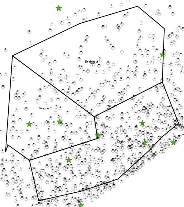
Going beyond getting directions, organizations large and small have discovered that mapping can be a great resource for analyzing patterns in data. By plotting the addresses of pizza lovers, a national pizza chain can visibly see where to locate the next grand opening. Political organizations planning on grassroots campaigns can easily see on a map where the undecided or unregistered voters are located and concentrate their route walks accordingly. While these mapping sites have given unprecedented power to interactive mapping, using them still requires that users gather point data and place it on the map. More critically, the reasoning that germinates from an interactive map is entirely visual. Back to the pizza example, the chain may be able to see the concentration of pizza lovers in a city or arbitrary sales region via visually inspecting their map showing pizza lovers by means of pushpins, but suppose we further differentiate pizza lovers by income level. If the chain has more of a gourmet offering, it would want to locate sites in the midst of mid- to high-income pizza lovers. They could use pushpins of different colors on the interactive map to indicate various income tiers, but the heuristic visual reasoning is now much more complicated, as shown in figure 1.1. Not only does the planner need to look at the concentration of pushpins, but she must keep the varying colors or icons of the pin in mind. Add another variable to the map, like households with more than two children, and the problem exceeds the processing power of the average human brain.
Figure 1.1. Pushpin madness!
Spatial databases can help solve this problem of information overload.
A spatial database is a database that defines special data types for geometric objects and allows you to store geometric data (usually of a geographic nature) in regular database tables. It provides special functions and indexes for querying and manipulating that data using something like Structured Query Language (SQL). A spatial database is often used as just a storage container for spatial data, but it can do much more than that. Although a spatial database need not be relational in nature, most of the well-known ones are.
A spatial database gives you both a storage tool and an analysis tool. Presenting data visually isn’t a spatial database’s only goal. The pizza shop planner can store an infinite number of attributes of the pizza-loving household, including income level, number of children in the household, pizza-ordering history, and even religious preferences and cultural upbringing (as they relate to topping choices on a pizza). More important, the analysis need not be limited to the number of variables that can be juggled in the brain. The planner can ask questions like “Give me a list of neighborhoods ranked by the number of high-income pizza lovers with more than two children.” Furthermore, she can add unrelated data such as location of existing pizzerias or even the health-consciousness level of various neighborhoods. Her questions of the database could be as complicated as “Give me a list of locations with the highest number of target households where the average closest distance to any pizza store is greater than 16 kilometers (10 miles). Oh, and toss out the health-conscious neighborhoods.”
Table 1.1 shows what the results of such a spatial query might look like.
Table 1.1. Result of a spatial query
|
Region |
#Households |
#Restaurants |
#Avg Travel |
|---|---|---|---|
| Region A | 194 | 1 | 17.1 km |
Suppose you aren’t a mapping user, but more of a data user. You work with data day in and day out, never needing to plot anything on a map. You’re familiar with questions like “Give me all the employees who live in Chicago” or “Count up the number of customers in each ZIP code.” Suppose you have the latitude and longitude of all the employees’ addresses; you could even ask questions like “Give me the average distance that each employee must travel to work.” This is the extent of the kind of spatial queries that you can formulate with conventional databases where data types consist mainly of text, numbers, and dates. Suppose the question posed is “Give me the number of houses within two miles of the coastline requiring evacuation in the event of a hurricane” or “How many households would be affected by the noise of a newly proposed runway?” Without spatial support, these questions would require collecting or deriving additional values for each data point. For the coastline question, you’d need to determine the distance from the beach house by house. This could involve algorithms to find the shortest distance to fixed intervals along the coastline or using a series of SQL to order all the houses by proximity to the beach and then making a cut. With spatial support all you need to do is to reformulate the question slightly as “Find all houses within a two-mile radius of the coastline.” A spatially enabled database can intrinsically work with data types like coastlines (modeled as linestrings), buffer zones (modeled as polygons), and houses (modeled as points).
As with most things worth pursuing in life, nothing comes without putting in some effort. You’ll need to climb a gentle learning curve to tap into the power of spatial analysis. The good news is that unlike other good things in life, the database that we’ll introduce you to is completely free.
If you’re able to figure out how to get data into your Google map, you’ll have no problem taking the next step. If you can write queries in non-spatially enabled databases, we’ll open your eyes and mind to something beyond the mundane world of numbers, dates, and strings. Let’s get started.
1.1.1. Introducing the geometry data type
The entirety of 2D mapping can be accomplished with three basic geometries: points, linestrings, and polygons. We can model physical geographical entities with these basic building blocks. This process is intuitive and interesting.
For example, an interstate highway crossing the salt flats of Utah clearly jumps out as linestrings. A salt flat can be represented by a polygon with a large number of edges. A desolate gas station located somewhere on the interstate can be a point.
You need not limit yourself to the macro dimensions of road atlases. Take your home; each room could be represented as a rectangular polygon, the wiring and the piping running from room to room could be linestrings, and the location of the doghouse in the back yard could be represented by a point. See how interesting this could be? Just by reducing the landscape to two-dimensional points, linestrings, and polygons, as shown in figure 1.2, you have the tools to model everything.
Figure 1.2. The basic geometries: a point, a linestring, and a polygon

Don’t be overly concerned with the rigorous definition of the geometries. Leave that for the mathematical topologists. Points, linestrings, and polygons are simplified models of reality. As such, they’ll never perfectly mimic the real thing. Don’t be overly concerned with geometries that you feel should be included but are missing. Two good examples are football stadiums and a beltway around a city. The former could be well represented by an ellipse; the latter could be modeled as a perfect circle. Both of these geometries aren’t defined (at least for now), but they could be approximated closely enough with polygons.
1.2. Modeling
We’ve introduced our building blocks of points, linestrings, and polygons. We’ve given an example of how to model real-world geographies using these basic geometries and have invited you to come up with your own. Modeling isn’t the only step in problem solving. Let’s go back to the salt flats of Utah. We know the interstate traverses the salt flats from one end to the other. A simple question that any motorist must be thinking would be “How long am I going to be on this thing?” Taking out a map, the driver may instruct her navigator to measure the distance from the mile marker where the interstate entered the salt flats to the mile marker where the interstate exits the salt flats, as shown in figure 1.3. Unbeknownst to the motorist, she has just formulated a spatial query.
Figure 1.3. The Utah salt flats—we can model them with linestrings, points, and polygons.

With our points, linestrings, and polygons in hand, let’s dissect this simple act of measurement and then see if we can ask it in a way that a spatially enabled database could easily answer. To start the measurement, the navigator looks for the point on the map where the interstate first hits the salt flats. This point is the intersection of the linestring with the polygon. The navigator then proceeds to find the place where the interstate leaves the salt flats and comes up with another point of intersection. Given that the highway is completely straight during its crossing of the salt flats, the navigator can use a ruler to measure from the first intersection point to the second intersection point. Let’s go through this with a higher level of abstraction. We start with two geometries: a linestring and a polygon. We overlay one atop the other and find the intersection of the two geometries. A line intersected with a polygonal area yields the linestring contained within the polygon. We finish by taking the length of the linestring.
One linestring through a polygon seems more like an exercise in geometry than a database query, but it’s the start of something powerful. Suppose the task at hand is to find the total length of all interstate highways in the state of Utah. We search for two tables: one with the polygons for all the states and one with all interstate highways in the United States, represented as linestrings. Next we extract the polygon that represents Utah from the states table and perform an SQL join with the highways table using the geometric intersects function as the join operator and geometric intersection as our output function. The output of that query would be those portions of all highways within the state of Utah. Finally, we aggregate those portions using the SQL LENGTH and SUM functions, and there’s our answer. With the Utah example we demonstrated that geometric data types and functions can leverage the querying power of a relational database and can easily lead to solutions for problems that at first sight looked insurmountable.
Don’t worry if you aren’t a whiz at SQL. When it comes to spatial databases, learning how to use the additional spatial functions is more important than being able to generate complex SQL statements. In our experience, simple SELECT, INSERT, and UPDATE statements will get you through 85% of the spatial queries that you’ll need to write.
1.2.1. Imagine the possibilities
We’ve demonstrated the power of spatial queries without telling you what a spatial query is or what it means to be spatial.
A spatial query is a database query that uses geometric functions to answer questions about space and objects in space. Spatial database extenders such as PostGIS add a body of functions to the standard SQL language that work with geometric objects in a database similar in concept to functions that work with dates. For example, with a date, you have functions that tell you how many hours/days/minutes/years/weeks are between two dates or whether this date is in the future or the past. For more sophisticated databases such as PostgreSQL, you can even define time and date intervals and answer with the overlaps function if two intervals overlap.
In addition to being able to answer questions about the use of space, spatial functions allow you to create and modify objects in space. This portion of spatial analysis is often referred to as geometric or spatial processing.
In the models we described previously we talked about points, linestrings, and polygons in two dimensions. These are the fundamental building blocks. In a spatially enabled database such as PostGIS/PostgreSQL, more complex objects exist such as MULTIPOLYGONS, MULTIPOINTS, MULTILINESTRINGS, GEOMETRYCOLLECTIONS, and curved geometries. In addition to the 2D world we’ve described, you can also have these 2D objects sitting in 3D space. This is often referred to as 2.5D and is the first step to real 3D modeling.
In the PostGIS 2 series of releases we’ll start seeing true 3D support in the form of polyhedral surfaces and triangulated irregular network (TIN) as well as relationship functions to work with 2.5D and 3D. Also introduced in PostGIS 2.0 is another kind of data called raster data. Raster data is data stored as individual pixel numeric values in bands and correlated with a location in space. Lots of useful information is coded in raster format. This allows analysis of things such as satellite weather data and digital elevation models (DEM) and overlaying these with vector data using SQL as well as slicing them up, creating derivatives, and overlaying them on a map. We’ll cover these more complex objects including the currently available PostGIS raster functionality in the later chapters of this book.
1.3. Introducing PostgreSQL and PostGIS
In the rest of this chapter, we’ll talk more about PostgreSQL and PostGIS. PostGIS is a free and open source (FOSS) library that spatially enables the free and open source PostgreSQL object-relational database management system (ORDBMS).
An object-relational database is one that can store more complex types of objects in its relational table columns than the basic date, number, and text and that allows the user to define new custom data types, new functions, and operators that manipulate these new custom types.
The major reason PostgreSQL was chosen as the platform on which to build PostGIS was the ease of extensibility it provided for building new types and operators and for controlling the index operators.
1.3.1. PostgreSQL strengths
PostgreSQL is an object-relational database system and has a regal lineage that dates back almost to the dawn of relational databases.
If you were to look at the family tree of PostgreSQL, it would look something like this:
System-R (1973)
   Ingres (1974)
          Postgres (1988)
              Illustra (1993)
                 Informix (1997)
                     IBM Informix (2001)
              Postgres95 (1995)
                 PostgreSQL (1997)
PostgreSQL is a cousin of the databases Sybase and Microsoft SQL Server because the people who started Sybase came from UC Berkeley and worked on the Ingres and/ or PostgreSQL projects with Michael Stonebraker. Michael Stonebraker is considered by many to be the father of Ingres and PostgreSQL and one of the founding fathers of object-relational database management systems. The source code of Sybase SQL Server was later licensed to Microsoft to produce Microsoft SQL Server.
PostgreSQL’s claim to fame is that it’s the most advanced open source database in existence. It has the speed and functionality to compete with the functionality of the popular commercial enterprise offerings and is used to power databases terabytes in size. Following are some of the compelling features that it has that most other open source databases lack and many commercial ones lack as well.
Postgresql Unique Features
PostgreSQL has many features that are rarely found in other databases. Some of its features don’t exist in other databases at all.
- Various languages to choose from for writing database functions that can return simple scalar values as well as data sets and for building aggregate functions— No open source or commercial database to our knowledge can compete with PostgreSQL in this regard. Commonly used ones are built-in SQL, PL/PGSQL, and C. In addition to the three built-in languages, PL/Perl, PL/Python, PL/TCL, PL/SH, PL/R, and PL/ Java are also often used. These require additional environment installs such as Perl, Python, TCL, Java, and R in order to take advantage of them. IBM DB2 and Microsoft SQL Server come close with allowing .NET functions, but this isn’t quite as elegant as being able to write the code right in the database. Oracle supports only PL/SQL and Java. In addition, the PostgreSQL PL platform is the most extensible of any database platform, making it easy register new language handlers. Watch for PL/Parrot, a procedural language handler for the Parrot system that allows for combining multiple dialects of languages in one procedural language.
- Support for arrays— PostgreSQL, Oracle, and IBM DB2 are fairly unique among databases in that arrays are first-class citizens. In PostgreSQL, you can define any table column as comprising an array of strings, numbers, dates, geometries, or even your own data type creations. This comes in handy for matrix-like analysis or aggregation. In addition, you can convert any single-column row list to an array, which is particularly useful when manipulating geometries.
- Table inheritance— PostgreSQL has a feature called table inheritance, which is something like object multi-inheritance. Table inheritance allows you to treat a whole set of tables as a single table as well as define nested inheritance hierarchies. It’s often used for table-partitioning strategies. We’ll demonstrate the power of this later.
- Ability to define aggregate functions that take more than one column— When you think of aggregates, you think of them as taking only one column as input. The multi-column feature isn’t commonly exploited and thus is hard to visualize. Multi-column aggregates have existed for some time in PostgreSQL. We have a couple of examples on our Postgres Journal site to demonstrate it: How to create multi-column aggregates: http://www.postgresonline.com/journal/archives/105-How-to-create-multi-column-aggregates.html Making SVG plots with PLPython and multi-column aggregates: http://www.postgresonline.com/journal/archives/107-PLPython-Part-5-PLPython-meets-PostgreSQL-Multi-column-aggregates-and-SVG-plots.html
Basic Enterprise Features
In addition to the unique features native to PostgreSQL, PostgreSQL also sports basic enterprise features that make managing mission-critical information easier.
- Exceptional ANSI-SQL compliancy, even when compared with the commercial offerings—Those familiar with working with other relational database systems should feel at home using PostgreSQL.
- A fairly sophisticated query planner and indexing support for complex objects that’s good for optimizing intricate joins and aggregations without the need for hints—The speed is comparable to enterprise-class DBMS for even the hairiest of SQL statements.
- Ability to define new data types fairly easily in both C and the built-in languages.
- Relational views with the ability to write rules against these that allows for updating even non-single table and rollup views.
- Advanced transactional support—It uses a multi-version concurrency control system, which is the same model that Oracle and Microsoft SQL Server 2005+ use. It also has features such as transaction save points.
- Thousands of built-in functions and contributed functions—These are for anything from string manipulation, regular expressions, and regression analysis to analysis of astronomical data.
- Similarity to PL/SQL—Those coming from an Oracle background will be surprised how similar Oracle’s PL/SQL language is to PostgreSQL’s native PL/ PgSQL. In addition to PL/PgSQL and numerous other languages, PostgreSQL has a built-in SQL function language, which other databases lack and which is much easier to write for simple set returning or calculation functions. Unlike other language functions, an SQL function isn’t a black box to the PostgreSQL planner. The major benefit of this is that it can be incorporated in the plan strategy. The logic is frequently in-lined in the query, similar to a macro in C. This makes it often more efficient than a PL/PgSQL or other language function while still hiding the complexity from the person utilizing the function.
- Ability to run on pretty much any OS you can think of.
- Ability to define column-level permissions, introduced in PostgreSQL 8.4.
- Ability to write variadic functions, also introduced in PostgreSQL 8.4—This allows you to write a single function that has a default argument if it’s not passed in. So getMyElephant('blue'), getMyElephant() would use the same function, but getMyElephant would use the default color defined in the function. PostgreSQL 9.0 extends the ways you can call functions by allowing named argument call notation similar to what you’ll find in languages like VB and Python: getMyElephant(color := 'blue').
Advanced Enterprise Features
In addition to the basic enterprise features PostgreSQL sports, it offers advanced enterprise features you’ll rarely find in other open source databases. Some of these features are also more advanced than the equivalent you’ll find in commercial database offerings.
- Ability to easily write your own aggregate function in most any supported language including SQL—This feature is particularly useful for something like spatial analysis. The simplicity and ease of writing aggregates will come as a shock for those who have come from other databases that allow this, but it require immense amounts of code to do it.
- Windowing functionality introduced in PostgreSQL 8.4— Many of the high-end commercial databases such as IBM DB2 and Oracle have had this functionality, and Microsoft SQL Server introduced it in its SQL Server 2005 offering. This is useful for OLAP and data warehouse applications and even more important for nearest-neighbor searches, as we’ll demonstrate. In PostgreSQL 9.0 this feature was enhanced to include numbered ROW RANGES, thus coming closer to the capabilities of Oracle’s windowing functionality and far surpassing SQL Server 2008 R2’s windowing functionality.
- Recursive common table expressions for writing recursive queries (useful for navigating trees) and common table expressions functionality, introduced in PostgreSQL 8.4—These are found in the popular high-end commercial databases. We’ll demonstrate how this functionality is particularly useful in spatial queries in the upcoming chapters. One important thing about this is that it follows the ANSI SQL 2003 standard, so it’s almost exactly what you’d write in Microsoft SQL Server and IBM DB2. Oracle has had its own variant for doing hierarchical queries almost since its inception called CONNECT BY that doesn’t follow the standard. Oracle introduced in its 11GR2 offering ANSI-compliant recursive common table expressions that follow the same CTE syntax as PostgreSQL, SQL Server, and IBM DB2.
- Database restore supports parallel restore of tables, introduced in PostgreSQL 8.4—This makes the database restore four times faster than it was in 8.3 and below, which is important for huge databases. In addition, the compressed backup storage format of PostgreSQL has always supported selective restore of objects.
- Column-level triggers and conditional triggers as well as simplified security management, introduced in PostgreSQL 9.0.
- Anonymous functions in any PL language via the new DO command, introduced in PostgreSQL 9.0—This allows for running Python, Perl, TCL, and PL/PgSQL code without defining a function.
- Built-in warm standby and streaming replication introduced in PostgreSQL 9.0.
- 64-bit support on Windows introduced in PostgreSQL 9.0.
- In-place upgrade introduced in PostgreSQL 8.4 and enhanced in later versions.
More Features in Postgresql 9.1
PostgreSQL 9.1 introduces many more sought-after features, both for enterprise and for ease of use.
- Support for ANSI SQL–compliant triggers on views.
- Enhancements to CTEs to support UPDATE/INSERT/DELETE.
- Functional dependency on foreign keys, which will simplify GROUP BY clauses by not requiring you to group by additional fields in a table if the primary key is already in the GROUP BY.
- CREATE TABLE IF NOT EXISTS similar to what MySQL has long had.
1.3.2. PostGIS, adding GIS to PostgreSQL
PostGIS is a project spearheaded by Refractions Research. PostGIS provides over 300 spatial operators, spatial functions, spatial data types, and spatial indexing enhancements. If you add to the mix the complementary features that PostgreSQL and other PostgreSQL-related projects provide, then you have one jam-packed powerhouse at your disposal that’s well suited for hard-core work as well as a valuable training tool for spatial concepts.
The power of PostGIS is enhanced by other supporting projects to include projection support (Proj4), advanced spatial operation support provided by the Geometry Engine Open Source (GEOS) project—a project ported from Vivid Solutions Inc.’s Java Topology Suite (JTS), historically incubated by Refractions Research and now a project of Open Source Geospatial Foundation (OSGeo). The foundation of PostGIS, the PostgreSQL object-relational database management system (ORDBMS), which provides transactional support, gist index support used to index spatial objects, and a query planner out of the box for PostGIS, is perhaps the most important of all. It’s a great testament to the power and flexibility of PostgreSQL that Refractions chose to build on top of PostgreSQL over any other open source database. It goes without saying that PostGIS would not be as useful today without the vast ecosystem that it leveraged and the ecosystem that has grown around it. This includes both open source and commercial tools that can work with it and numerous toolkits and application frameworks that use it as a core data storage and manipulation tool.
OGC stands for Open Geospatial Consortium and is the body that exists to try to standardize how geographic and spatial data is accessed and distributed. In that mission, they have numerous specifications that govern accessing geospatial data from web services, geospatial data delivery formats, and querying of geospatial data.
OSGeo stands for Open Source Geospatial Foundation and is the body whose initiative is to fund, support, and market open source tools and free data for GIS. There is some overlap between the two. Both strive to make GIS data and tools available to everyone, which means they’re both concerned about open standards.
If your data and your APIs can be accessed by standards available to everyone—people using Cadcorp, Safe FME, AutoCAD, Manifold, MapInfo, ESRI ArcGIS, OGR2OGR/ GDAL, OpenJUMP, Quantum GIS, deegree, UMN MapServer, GeoServer, MapDotNet, and the like—then everyone can use the tools they feel most comfortable with or fit their work process and/or can afford and share information with one another. OSGeo tries to ensure that regardless of how big your pocketbook is, you can still afford to view GIS data. OGC tries to enforce standards across all products so that regardless of how expensive your GIS platform is, you can still make your hard work available to all constituents. This is especially important for government agencies whose salaries and tools are paid for with tax dollars, students who have a lot of will and the intelligence to learn and advance technology but have small pockets, and even smaller vendors who have a compelling offering for specific kinds of users but who are often snubbed by larger vendors in the market because they can’t support or lack access to private API standards of the big-name vendors in the industry.
PostGIS and PostgreSQL also conform to industry standards more closely than most products. PostgreSQL supports most of ANSI SQL 92-2003+ and some of ANSI SQL 2006. PostGIS supports OGC standards SQL/MM Spatial (ISO JTC1, WG4, 13249-3). This means that you aren’t simply learning how to use a set of products; you’re garnering knowledge about industry standards that will carry you through grasping other commercial and open source geospatial databases and mapping tools.
PostGIS carries less baggage than most other spatial database engines. The fact that you can see the code and how it works makes it an ideal training tool for teaching spatial database concepts and also makes it easier to troubleshoot when things go wrong.
PostGIS has numerous functions you won’t find even in the commercial offerings. In general it has more output formats than the commercial offerings and its speed is on par with and sometimes better than the commercial ones for common spatial needs.
1.3.3. Alternatives to PostgreSQL and PostGIS
Admittedly, PostGIS/PostgreSQL isn’t the only spatial database in existence. Most of the high-end commercial relational database systems provide spatial functionality. The first two to do that were Oracle (with its included Locator, priced add-on Oracle Spatial, and before those its spatial data option (SDO)), IBM DB2 and IBM Informix (with their add-on priced options Spatial DataBlade and Geodetic DataBlade). Recently SQL Server 2008 provided spatial functionality with its built-in Geometry and Geodetic Geography types and companion spatial functions. Ingres, the older cousin of PostgreSQL, is also enhancing its spatial support, using some of the same plumbing that underlies PostGIS. The new kid on the block is SpatiaLite, which is an add-on to the open source SQLite portable database. SpatiaLite is especially interesting because it’s well positioned to be used as a low-end companion to PostGIS and other high-end spatially enabled databases. It can be used to create master/slave applications to provide basic lightweight spatial support for clients such as portable devices. It also has a companion, RasterLite, that’s for the most part focused on raster data storage and display and so makes a great companion to the raster analysis that’s being developed in PostGIS. SpatiaLite and RasterLite also use many of the core libraries that PostGIS uses: GEOS, PROJ, and GDAL. This fact makes it an even more fitting companion to PostGIS, because many of the conventions are the same and much of the ecosystem around PostGIS also supports or is starting to support SpatiaLite/RasterLite. What SpatiaLite lacks is a strong enterprise database behind it that allows for writing advanced functions and spatial aggregate functions. That’s why some spatial queries possible in PostGIS are harder to write or not even possible in SpatiaLite. SpatiaLite’s single file and embedded engine make it less threatening and easier to deploy for users new to databases or GIS.
MySQL has had spatial support for quite some time, but its spatial development is fairly stagnant and even weaker than that of SpatiaLite. Now that it’s a property of Oracle, it’s questionable how interested Oracle will be in beefing up MySQL spatial support, because this competes directly with its Oracle Locator/Spatial offering. MySQL 4 and 5 have built-in spatial functionality, with one major drawback: Their geometric functions have until now worked only with the bounding boxes of geometries and did not provide indexed access (except for MyISAM stored tables). Only recently, before the Oracle acquisition (and still not released in production), has MySQL started to add functions that work against real geometries rather than just the bounding box caricatures.
In addition to the spatial functionality provided by the popular commercial database vendors, Environmental Systems Research Institute (ESRI) has for a long time provided its spatial database engine (SDE) with its ArcGIS product. The SDE engine is integrated into the ArcGIS line of products and was often used to spatially enable external databases such as Microsoft SQL Server 2005 and below that lacked spatial functionality. It also often competes with and, some would say, castrates the built-in spatial functionality of existing databases such as PostgreSQL, Oracle, or Microsoft SQL Server 2008, because in order to use the ST_Geometry type and functions that ArcGIS provides, you need to go through the middleware layer of ArcGIS Server.
1.3.4. What works with PostGIS
The following commercial vendors currently support PostGIS in their desktop/web offerings. In later chapters we’ll go over the free and open source GIS tools that support PostGIS as well.
- Cadcorp SIS— This vendor is partially funding the raster support in PostGIS and is a favorite among modelers for both desktop and web-based apps. Cadcorp supports more than 160 formats, including direct support for all other high-end spatial database offerings.
- Safe FME— It contributes both monetary and developer support for GEOS and makes extract transform load (ETL) tools for GIS data, which makes moving GIS data transport to different formats and databases a simple drag, drop, and schedule exercise. It’s the favorite for high-end ETL transactions.
- Manifold— It released support for PostGIS in its version 8.0 and above product, and it’s a favorite of many spatial database analysts and people who like SQL in all its glory (it supports Oracle Locator/Spatial, PostGIS, SQL Server 2008, IBM DB2, MySQL, and its own extender for SQL Server 2005).
- zigGIS— This is a desktop plug-in for the ESRI ArcGIS desktop that works with 9.2 and above and allows you to access PostGIS data without an ArcSDE license. It doesn’t work with ArcGIS Server as of this writing.
- ArcGIS— In ArcGIS 9.3, ESRI introduced support for PostGIS. Although this requires an ArcSDE Server license for PostGIS and works only with PostGIS 1.4 and below (as of ArcGIS 10), it may not be suitable for people on a limited budget or who want to use more recent versions of PostGIS or PostgreSQL. ArcGIS is best known for its cartography. See http://resources.arcgis.com/content/arcsde/10.0/postgresql-system-requirements.
- Pitney Bowes MapInfo 10— Pitney Bowes introduced support for PostGIS in its recent MapInfo 10 offering. MapInfo is a popular tool for GIS VB programmers using its MapBasic interface. It enjoys a rich history of integration with MS Office products. It’s a favorite of lightweight GIS users and database analysts because of its rich query options and easy data import menus.
Its commercial vendor support is now just as strong as what you’ll find available for Oracle, SQL Server, or IBM DB2. PostGIS has garnered more support in the free open source GIS arena than any other spatial database, far exceeding the spatial offerings of MySQL. There are too many PostGIS open source tools to list. We’ll cover the more common offerings in our desktop and web tools chapters. As you can see, PostGIS has an already strong and growing commercial support belt as well.
1.4. Getting started with PostGIS
In this section we’ll show some simple examples for creating geometries with PostGIS; in later sections of this chapter we’ll cover loading and querying spatial data. Before going further, you’ll need to have a working copy of PostGIS 1.3 or higher and PostgreSQL 8.2 or higher, as well as ancillary tools such as pgAdmin III to compose and execute your queries. Information about acquiring and installing these can be found in appendix B. As always, if you’re starting completely from scratch, we recommend that you install the latest versions.
pgAdmin III is the free administrative GUI that comes packaged with PostgreSQL. It can also be downloaded from http://www.pgadmin.org/ and installed separately on any client computer. Precompiled binaries are available for most operating systems. pgAdmin III 1.9 and above support a plug-ins architecture, which allows you to call shp2pgsql-gui and any other executables you like from within pgAdmin. The psql command-line client is packaged with it as a plug-in. All this is configurable by editing the plugins.ini file.
1.4.1. Verifying version of PostGIS and PostgreSQL
If you’d like to see the geometries visually, we recommend that you install one of the desktop utilities available for working with PostGIS that we describe in chapter 12. For most of these exercises we use OpenJUMP for visualization. For detailed installation guides on PostgreSQL, PostGIS, and pgAdmin III, please refer to appendix B. The following examples require PostGIS 1.3 or above and PostgreSQL 8.2 or above. In later sections, we’ll be using some features introduced in PostgreSQL 8.4 and PostGIS 1.5.
Execute the following query in pgAdmin III to verify that you have PostGIS installed successfully and to obtain the version number:
SELECT postgis_full_version();
If all is well, you should see the version of PostGIS, the GEOS library, and the PROJ Library installed along with PostGIS displayed, as shown here:
POSTGIS="1.5.2" GEOS="3.2.2-CAPI-1.6.0" PROJ="Rel. 4.6.1, 21 August 2008"
LIBXML="2.7.6" USE_STATS
Run the following to verify what version of PostgreSQL you’re running:
SELECT version();
If all is well, you should see the PostgreSQL version and operating system:
PostgreSQL 8.4.2, compiled by Visual C++ build 1400, 32-bit
1.4.2. Creating geometries with PostGIS
We’ll get started creating points.
Points
To create a point at (X,Y), type the following line into your query builder:
SELECT ST_Point(1, 2) AS MyFirstPoint;
Not much to it, is there? We didn’t specify a spatial reference system for our simple point. The default coordinate system type used is the basic Cartesian grid you learned in childhood. In most real-world applications, you’ll need to be explicit about the spatial reference system being used.
A spatial reference system is a way of denoting the coordinate system that’s used to define geometry points. This is a bit of a simplistic definition but will do for now. You can be assured that if two geometries are in the same spatial reference system, they can be overlaid without distortion. PostGIS packages about 3,000 of these, and these are all denoted by numbers (currently just European Petroleum Survey Group (EPSG) standard codes that are common in the industry) and can be looked up in the included spatial reference table. They define how geographic data is represented on a flat map and what units of measurement (degrees, feet, meters) the coordinate system uses. Spatial reference systems are in general good for only a specific region of the globe.
With this in mind, let’s create yet another point that has real geographical relevance:
SELECT ST_SetSRID(ST_Point(-77.036548, 38.895108),4326);
Here we added a function to indicate that our point is using a spatial reference system known as WGS 84 Lon Lat. This refers to the longitude and latitude that most people are familiar with. Incidentally, this point is the Zero Milestone in Washington, D.C. When the United States was a young (and small) nation, the city planners of the day intended all distances to be measured from this point. You can read more about it at http://en.wikipedia.org/wiki/Zero_Milestone.
The function ST_GeomFromText offers a more generic method for creating various geometry types from a textual representation. This function is slower and less accurate than the ST_Point function, but it’s intuitive and applies to all geometric types. Here’s how you’d create a point with ST_GeomFromText:
SELECT ST_GeomFromText('POINT(-77.036548 38.895108)', 4326);
This approach can be used to create any geometry with what is called well-known text (WKT) representation of a geometry.
Well-known text representation is an OGC standard for representing geometries as text. ST_AsText and ST_GeomFromText are OGC functions found commonly in many OGC-compliant spatial databases that convert back and forth between a database’s native binary format to a textual display format.
You should have noticed that the result of this geometry constructor would look like this:
0101000020E6100000FD2E6CCD564253C0A93121E692724340
Most spatial databases store geometries in some a binary format that’s impossible for the eye to make heads or tails of. This is why most spatial databases have functions to reformat the native binary format to WKT. In PostGIS, this is the ST_AsEWKT function. Try formatting the previous PostGIS binary format using this function:
SELECT ST_AsEWKT('0101000020E6100000FD2E6CCD564253C0A93121E692724340'),
You’ll end up with the more readable WKT-like representation of
SRID=4326;POINT(-77.036548 38.895108)
A variant of the ST_AsEWKT function is ST_AsText. This function returns the commonly accepted WKT format, which doesn’t include the spatial reference identifier.
You’ll note that the points are stored in longitude, latitude and not latitude, longitude. This storage is common for spatial databases. Most people are used to thinking in latitude, longitude, so one of the more common mistakes people make is flipping these coordinates and ending up in Antarctica when they mean Washington, D.C.
Linestrings and Polygons
Now let’s move on to more complex examples of creating linestrings and polygons. PostGIS is primarily used to store and query geographic data, but we can also use PostGIS to represent any data that can be drawn using a Cartesian coordinate system. We’ll start by creating a linestring without specifying a spatial reference system. We’ll use the ST_GeomFromText function without the spatial reference parameter to create the geometries shown in figure 1.4.
Figure 1.4. Linestrings and polygons created in the following code snippets

SELECT ST_GeomFromText('LINESTRING(-14 21,0 0,35 26)') AS MyCheckMark;
This creates a check mark–like linestring through the origin. As you may be able to observe, a linestring is nothing more than a sequence of points. How about a heart with jagged edges?
SELECT ST_GeomFromText('LINESTRING(52 218, 139 82, 262 207, 245 261, 207 267,
     153 207, 125 235, 90 270, 55 244, 51 219, 52 218)') AS HeartLine;
The syntax for creating a polygon is similar to that of the linestring. The key difference is that the polygon must use closed linestrings, also known as rings. As you might have already guessed, a closed linestring is a linestring where the starting point coincides with the end point. Our heart linestring in the figure is closed. To draw a polygon, we specify the linestring forming its boundary. Here’s a triangle:
SELECT ST_GeomFromText('POLYGON((0 1,1 -1,-1 -1,0 1))') As MyTriangle;
Because our heart is closed, we can use it as the boundary for a heart polygon. Our heart polygon would include all the interior points of the geometry as well as the original linestring forming the boundary:
SELECT ST_GeomFromText('POLYGON((52 218, 139 82, 262 207, 245 261,
 207 267, 153 207, 125 235, 90 270,
  55 244, 51 219, 52 218))') As HeartPolygon;
The first interesting thing about the WKT representation of a polygon is that it has one additional set of parentheses that a linestring doesn’t have. Why is this? A polygon can have holes, and each hole needs its own set of parentheses. Our triangle and our heart happen to not have any holes, so the extra parentheses appear redundant. When we explore polygons in detail in the next chapter, we’ll show you how to create donut-like polygons.
Now that we’ve covered the basics of geometry creation, we’ll cover the more common case of loading preexisting spatial data from other sources and querying the loaded data.
1.5. Working with real data
In this section, we’ll cover how to load data from the two most common formats: delimited ASCII data and ESRI shapefile data. For delimited data, we’ll demonstrate how to convert those to spatial points, using the lessons you learned in the previous section. For shapefile data, we’ll load a data file of road linestrings, using the ESRI shapefile loader packaged with PostGIS.
When working with PostGIS, you often start off by loading data either from a flat file delimited format or a spatial format and then perform various operations on it to get it into a structure suitable for spatial querying. A common task is to convert plain-text representations of a location, like longitude/latitude coordinates, into spatial data types such as geometry or geography. For geometry data, we often need to transform lon lat values to a planar-based spatial reference system that’s suitable for planar measurement.
Data in the geography data type must always be stored in WGS 84 Lon Lat degrees. However, all measurements in geography are expressed in meters. If your source data is in a planar coordinate system such as State Plane feet or meters, and you want to use the geography data type for storage, you must load it as geometry, transform it, and then cast it to geography.
Geometry data, on the other hand, can be stored in any spatial reference system. The measurements are always in the units of that spatial reference system. This means if your data is lon lat, your measurements will be in degrees. This isn’t useful for most kinds of analysis, so for geometry data, people often transform their data to a measurement that preserves the spatial reference system that’s valid for their area of interest. Some common ones are UTM zones meter and State Plane feet or meters, and there are thousands more. We’ll cover the nuances of this in later chapters and explain how to choose a suitable spatial reference system.
If you’re new to GIS or SQL, many of the terms and syntax we use in this section will be foreign to you. This is a crash course. Don’t worry if you don’t completely understand what’s going on. These processes will be repeated in later chapters and become clearer when you see them again.
1.5.1. Loading comma-separated data
We’re going to start off by loading point data from a comma-delimited flat file. It’s a list of fast-food restaurants generously provided to us by fastfoodmaps.com. The tools you need to accomplish this are available in PostgreSQL and apply to loading any kind of data in PostgreSQL.
Before we load in data, we create the schema and table to house our data. In listing 1.1 we also create a lookup table for the franchises so we don’t have to remember the codes. The table we create should have the same column ordering and preferably the same number of columns as the data we’ll be loading.
Listing 1.1. Set up fastfoods and franchises lookup
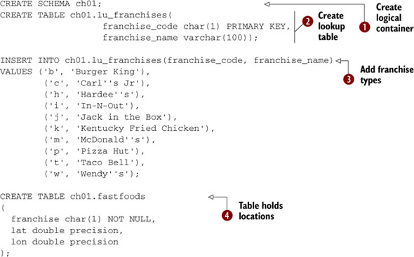
![]() First we create a schema to hold our data. A schema is a container you’ll find in most high-end databases. It logically segments
objects (tables, views, functions, and so on) for easier management. Refer to appendix D for more details.
First we create a schema to hold our data. A schema is a container you’ll find in most high-end databases. It logically segments
objects (tables, views, functions, and so on) for easier management. Refer to appendix D for more details. ![]() Next we create a lookup table to map franchise codes to meaningful names
Next we create a lookup table to map franchise codes to meaningful names ![]() . We then add all the franchises we’ll be dealing with
. We then add all the franchises we’ll be dealing with ![]() . Finally, we create a table to hold the data we’ll be loading. We define only columns that are in our source dataset. We’ll
add additional columns after the load.
. Finally, we create a table to hold the data we’ll be loading. We define only columns that are in our source dataset. We’ll
add additional columns after the load.
There are two common ways you can copy flat file data into PostgreSQL. You can use the built-in SQL function called COPY or use the psql copy command. The SQL function requires that the Postgres daemon process have access to the data path and also requires that you be logged in as a PostgreSQL super user. Other databases have similar SQL constructs. For example, in SQL Server you use the BULK INSERT SQL construct.
When using the SQL COPY function, the path is relative to the server. You can run the SQL COPY function anywhere you can run SQL. This can be in a .NET or PHP app, pgAdmin III, psql, or some other third-party database client tool.
The psql copy command, on the other hand, is a client-side feature built into the PostgreSQL-packaged psql command-line tool. It requires that the computer you’re running psql on have access to the file path and also that your OS account have access to read the file. The path is relative to the client computer. We offer a more thorough description of these distinctions on our Postgres Journal site: http://www.postgresonline.com/journal/index.php?/archives/157-Import-fixed-width-data-into-PostgreSQL-with-just-PSQL.html.
Using the SQL command method, we’d do the following. Note that when we use the SQL COPY command, the /data/ path references the path on the PostgreSQL server:
COPY ch01.fastfoods FROM '/data/fastfoods.csv' DELIMITER ',';
Using psql, the command-line tool, we’d do the following, and the path would reference the folder on our local computer from which we started psql:
copy ch01.fastfoods from '/data/fastfoods.csv' DELIMITER AS ','
After we’ve finished loading data, we add a primary key to the table so we can uniquely identify each fast-food restaurant:
ALTER TABLE ch01.fastfoods ADD COLUMN ff_id SERIAL PRIMARY KEY;
The easiest way to access the psql command line is via the Plugins menu icon in pgAdmin III. To do so, select a database you want to connect to and then click the PSQL Console menu option.
1.5.2. Spatializing flat file data
Until now, our lon lat values have been plain database numbers. We need to convert these numbers into either geometry or a geography data type in order to take advantage of PostGIS’s spatial functionality.
If you’re using PostGIS 1.4 or lower, you can choose only the geometry data type. With PostGIS 1.5 or above, you have the additional option of the geography data type. The advantage of the geography data type is that it returns measurements in meters and allows you to store data using longitude, latitude degree values. This means that you can cover the whole world with geography data and never have to learn anything about spatial reference systems and projections. The disadvantage of geography is that for localized areas, it may not be as precise as using a geometry type. Also, fewer functions are available for it than for geometry. The speed of functions such as ST_Intersects and other relationship functions for geography is currently lower than for the geometry data type, though this will change in time. On the other hand, it’s fairly easy to convert between these two spatial types.
Those who have worked with SQL Server 2008 spatial types may recognize the similarity in naming. The similarity extends beyond nomenclature to include functionality as well. The SQL Server 2008 geometry type is an OGC type similar to the PostGIS OGC geometry type. Just like the PostGIS geometry type, the SQL Server 2008 geometry type treats all data as planar data. PostGIS and SQL Server geography data types aren’t OGC types, though they try to follow many of the same function and naming conventions as OGC geometry functions. OGC is mainly concerned with planar geometries and operations. The PostGIS geography type was inspired by the SQL Server 2008 geography data type. Both geography types measure data along an ellipsoid instead of a Cartesian plane. Where they’re different is that SQL Server 2008 doesn’t have built-in support for transformation from one spatial reference system to another for its geometry data type, whereas PostGIS has robust support for this for its geometry datatype. As for geographies, SQL Server 2008 supports many lon lat–based spatial reference systems. PostGIS geography currently supports only EPSG:4326, also referred to as WGS 84 Lon Lat. WGS 84 Lon Lat is the most common spatial reference system for longitude latitude data.
In these next examples we’ll demonstrate how to define a geometry point data type in our fastfoods table, update data to populate this new column, and then repeat the exercise using the geography data type.
Using the Geometry Data Type
If we were to use the geometry data type, we’d do the following.
Listing 1.2. Using the geometry data type to store data

![]() We first add a geometry column to the fastfoods table to house our future spatial points.
We first add a geometry column to the fastfoods table to house our future spatial points. ![]() Because geometry is a planar projection, we want our points to be in a projected coordinate system that covers our area of
interest. We’ve picked EPSG:2163, which is an equal area projection covering the continental United States. The measurements
of its coordinate system are in meters and are a little less accurate when modeling the earth as a sphere.
Because geometry is a planar projection, we want our points to be in a projected coordinate system that covers our area of
interest. We’ve picked EPSG:2163, which is an equal area projection covering the continental United States. The measurements
of its coordinate system are in meters and are a little less accurate when modeling the earth as a sphere. ![]() The PostGIS ST_Transform takes our data from lon lat degrees and projects it to North American Equal Area. The main drawback
of this particular spatial reference system is that because it covers a fairly large area, measurements will less accurate
than if we had used geography, which by default assumes a spheroid model of the earth. Speed will be faster and we’ll be free
to use the vast array of geometry functions. We then
The PostGIS ST_Transform takes our data from lon lat degrees and projects it to North American Equal Area. The main drawback
of this particular spatial reference system is that because it covers a fairly large area, measurements will less accurate
than if we had used geography, which by default assumes a spheroid model of the earth. Speed will be faster and we’ll be free
to use the vast array of geometry functions. We then ![]() do some general housecleaning by creating a spatial index on our new column.
do some general housecleaning by creating a spatial index on our new column.
Using the Geography Data Type
If we were to use the geography data type, we’d do the following with our data.
Listing 1.3. Using the geography data type to store data

In this example we explicitly use SRID=4326 in our construction. We do this for clarity and also in case PostGIS in the future supports more spatial reference systems for geography. In practice, you can leave it out and PostGIS will assume 4326.
The steps we follow for creating geography columns are similar to what we did for geometry, but there are some differences.
![]() Geography uses the built-in typmod feature introduced in PostgreSQL 8.3 (this is the main reason why you can’t install PostGIS
1.5 on anything lower than 8.3). This allows adding constrained geography columns without the need for an AddGe.. function.
Geography uses the built-in typmod feature introduced in PostgreSQL 8.3 (this is the main reason why you can’t install PostGIS
1.5 on anything lower than 8.3). This allows adding constrained geography columns without the need for an AddGe.. function.
![]() Instead of using ST_GeomFromText, we use the parallel ST_GeogFromText, but the WKT representation is more or less the same.
Because geography measures along a spheroid rather than a plane, we don’t need to transform to get meaningful measurements.
Instead of using ST_GeomFromText, we use the parallel ST_GeogFromText, but the WKT representation is more or less the same.
Because geography measures along a spheroid rather than a plane, we don’t need to transform to get meaningful measurements.
![]() As we did with geometry, we create our spatial index.
As we did with geometry, we create our spatial index.
It’s good to follow up any bulk load process with a vacuuming:
vacuum analyze ch01.fastfoods;
The vacuum-analyzing step is a process that gets rid of dead rows and updates the planner statistics. It’s good practice to do this after bulk uploads. If not done, the vacuum daemon process, which is enabled by default, will eventually do it for you.
Adding Constraints
Our fast-foods data has no primary key index. Unfortunately, nothing in the data file lends itself to a good natural primary key. For our later analysis, we’ll need to uniquely identify restaurants so that we don’t double-count them. Also certain mapping applications and viewers, such as QGIS and MapServer, have issues with tables without primary keys. They also complain if that primary or unique key isn’t an integer. So we’ll create an autonumber primary key on our fastfoods table.
ALTER TABLE ch01.fastfoods ADD COLUMN ff_id SERIAL PRIMARY KEY;
Although not necessary for this particular data set because it won’t be updated, we’ll create a foreign key relationship between our fastfoods franchise column and our lookup table. This helps prevent people from introducing franchises we don’t know about in our restaurants table. Adding CASCADE UPDATE DELETE rules when we add foreign key relationships will allow us to change the franchise codes for our franchises if we want and have those update the fastfoods table automatically. By restricting deletes, we can prevent people from inadvertently removing franchises with extant records in the fastfoods table. One added benefit of foreign keys is that relational designers such as what you’ll find in OpenOffice Base and other ERD tools will automatically draw lines between the two tables to visually alert you to the relationship.
ALTER TABLE ch01.fastfoods
        ADD CONSTRAINT fk_fastfoods_franchise
        FOREIGN KEY (franchise)
        REFERENCES ch01.lu_franchises (franchise_code)
   ON UPDATE CASCADE ON DELETE RESTRICT;
We then create an index to make the join between the two tables a bit more efficient:
CREATE INDEX fki_fastfoods_franchise ON ch01.fastfoods(franchise);
All this code was autogenerated by using the pgAdmin GUI. There isn’t any need to memorize how to do this in SQL, although it’s standard Data Definition Language (DDL) code across many relational databases.
1.5.3. Loading data from spatial data sources
The most common spatial format that data is distributed in is the ESRI shapefile format. In PostGIS 1.5 and above, a GUI tool called shp2pgsql-gui makes loading this kind of data simple and user friendly. It can also be used as a plug-in to pgAdmin III. Details on how to install and get started with it are provided in appendix B. It’s packaged with the Windows Stack Builder installs as well as the OpenGeo Suite 1.9+ GIS stack installs.
When shp2pgsql-gui is used as a plug-in in pgAdmin III, it reads your database credentials directly from pgAdmin III for the selected database. Even if you’re using a version of PostGIS below 1.5, you can still use this tool against a PostgreSQL 8.2 or higher with PostGIS 1.3 or higher version installed. You can even use the DBF-only loader portion on a database without PostGIS.
For our next example we’ll use shp2pgsql-gui. to demonstrate loading the road network data we downloaded from http://www.nationalatlas.gov/atlasftp.html#roadtrl. For this example we’ll be going through pgAdmin and accessing from the Plugins menu, as shown in figure 1.5.
Figure 1.5. The Plugins menu of pgAdmin III shows the PostGIS Shapefile and DBF loader.
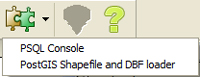
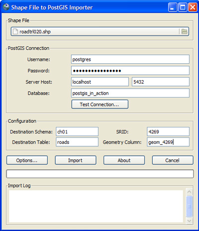
The Plugins option will be disabled until you select a database from the pgAdmin database tree. When you click the PostGIS Shapefile and DBF Loader menu option, the dialog box shown in figure 1.6 comes up with the credentials of the selected database already filled in.
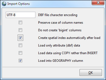
Figure 1.6. Loading into the geometry data type

If you don’t have shp2pgsql-gui available, you can load the data using the command-line loader shp2pgsql. Shp2pgsql is included with all PostGIS packages for all versions of PostGIS. The equivalent command using shp2pgsql is
shp2pgsql -s 4269 -g geom_4269 /data/roadtrl020.shp ch01.roads | psql -h localhost -U postgres -p 5432 -d postgis_in_action
Loading Data into the Geometry Data Type
In order to load into the geometry data type, you must browse to the file. Make sure to indicate that you’ll be loading into the ch01 schema and into a new table called roads. Shp2pgsql-gui will create the table for you. Note that we also changed the default geometry column name to geom_4269. Click the Options button and uncheck Create Spatial Index Automatically After Load, and make sure Load Into GEOGRAPHY Column is unchecked. Normally you’d want a spatial index created when loading data, but in this case we don’t because geom_4269 is a temporary column that we’ll be dropping once we’ve finished with it. Suffice for now that the road data is in a lon lat spatial reference system called North American Lon Lat Datum 1983 (4269), which is similar to WGS 84 Lon Lat (4326). They’re so similar that in most cases you can treat them the same. When you’ve finished setting the options, click the Import button.
Neither WGS 84 Lon Lat nor NAD 83 Lon Lat is useful for measurement in geometry type. They would get squashed into a rectangular planar grid where the X axis would be longitude and Y axis would be latitude. This “rectangularization” is often referred to as a Plate Carrée projection. The other reason won’t be using lon lat in geometry is that the measurements would return degrees. Unless you’re a mariner, degrees of longitude and latitude probably don’t mentally translate well into distance measures. That being said, in listing 1.4 we’ll transform this column into the same spatial reference system we’re using for our fast-foods data so that it will be useful for doing spatial comparisons between them and being able overlay them both on the same map without distortion.
Listing 1.4. Using the geometry data type to store roads data
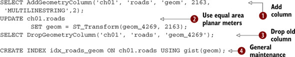
In order to load the roads data into the geometry data type format, we use shp2pgsqlgui to load it into its native spatial
reference system. Neither the shp2pgsql command line nor the GUI has transformation abilities. To make the input suitable
for measurement, we transform it after we’ve loaded it in the database. To do so, ![]() we add a new column that holds a Cartesian spatial reference that covers our area of interest and is suited for doing measurements
we add a new column that holds a Cartesian spatial reference that covers our area of interest and is suited for doing measurements
![]() . We update this new column by transforming our imported geometry data to the new spatial reference system
. We update this new column by transforming our imported geometry data to the new spatial reference system ![]() . After that, we no longer need the original column, so we drop it.
. After that, we no longer need the original column, so we drop it. ![]() Then we do our usual creating an index.
Then we do our usual creating an index.
After you’ve finished loading data, it’s good to follow up with a vacuum analyze so statistics are up to date:
vacuum analyze ch01.roads;
In the next example, we’ll repeat the same exercise, but we’ll load into the geography data type.
Loading Spatial Data into the Geography Data Type
For this particular data set, loading into the geography data type is much simpler than loading into geometry. The reason is that our data is already in lon lat units, and although NAD 83 Lon Lat isn’t the same as WGS 84 Lon Lat, we can pretend it is because for most areas the differences are extremely small. Remember that not all lon lat data can be treated as similar. For instance, NAD 27 Lon Lat (4267) is sufficiently different that you would have to bring your in data as geometry, transform it to 4326, and cast it to geography—something along the lines of geography(ST_Transform (geom_4267,4326)).
We use the loader, as shown in figure 1.7, to ease the import.
Figure 1.7. Loading data into the geography data type. We pretend our data is 4326 instead of 4269 because they’re similar. We go ahead and index and check the load into geography.

As you can see in the figure, our settings are more or less the same as those we chose for geometry, except that we chose to create the index, load into geography, and load into a different table, roads_geog. We also changed the name of the column so we know it holds geography data type data instead of geometry. The equivalent command using shp2pgsql is
shp2pgsql -G -g geog /data/roadtrl020.shp ch01.roads_geog | psql -h localhost -U postgres -p 5432 -d postgis_in_action
There’s nothing else we need to do after this except to vacuum analyze ch01.roads_geog.
1.6. Using spatial queries to analyze data
Now that we have spatial data loaded in our database, we’re able to spatially analyze this data with standard statistical SQL queries, yielding just raw numbers and text, as well as with queries returning geometric objects that can be rendered on a map. We’ll start off by doing statistical queries to count restaurants by their proximity to roads and to determine which roads have the largest number of restaurants.
Before we got to this point, we transformed all the disparate data sets into a common planar spatial reference system, in this case North America Equal Area Meter (2163). Because we chose a meter-based reference, all our units are in meters. When we ask questions using miles, keep in mind that the conversion factor of 1609 meters equal one mile.
1.6.1. Proximity queries
One of the most common uses of PostGIS and other spatial databases is to compute the proximity of objects to each other. For the next couple of examples, we’ll demonstrate how to combine the ST_DWithin function of PostGIS with standard SQL operations like COUNT, JOINS, and GROUP BY.
How Many Fast-Food Restaurants by Chain are Within One Mile of a Main Highway?
For this case, we answer the question and also order our results by the number of restaurants by franchise, with the most numerous being at the top. Although we’re using the geometry type in the following listing, the query itself would be written exactly the same for a geography column because an ST_DWithin function is available for both geometry and geography types.
Listing 1.5. List franchise name, count of restaurants on a principal highway

In this example we ![]() use an ANSI-SQL COUNT(DISTINCT) construct to ensure we count a fast-food restaurant only once even if it’s within a mile
of more than one highway segment.
use an ANSI-SQL COUNT(DISTINCT) construct to ensure we count a fast-food restaurant only once even if it’s within a mile
of more than one highway segment. ![]() We use a regular non-spatial join with our lookup table to grab the meaningful name of the franchise.
We use a regular non-spatial join with our lookup table to grab the meaningful name of the franchise. ![]() We use a spatial join between fastfoods and roads to pick up only restaurants within one mile of a principal highway, which
gives us this:
We use a spatial join between fastfoods and roads to pick up only restaurants within one mile of a principal highway, which
gives us this:
| franchise_name | tot |
| McDonald's | 5343 |
| Burger King | 3049 |
| Pizza Hut | 2920 |
| Wendy's | 2446 |
| Taco Bell | 2428 |
| Kentucky Fried Chicken | 2371 |
| : |
Which Highway has the Largest Number of Fast-Food Restaurants Wit- thin a Half-Mile Radius?
In this next example we’ll demonstrate a slight twist to the earlier example and determine which highway has the highest number of restaurants along a half-mile boundary.
Listing 1.6. Return the principal highway that has the most restaurants and how many
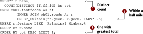
![]() Because we’re joining with a roads table with multiple records, it’s possible for a restaurant to be within a half mile of
more than one record, so we use the SQL DISTINCT clause to prevent double-counting.
Because we’re joining with a roads table with multiple records, it’s possible for a restaurant to be within a half mile of
more than one record, so we use the SQL DISTINCT clause to prevent double-counting. ![]() We use the PostGIS ST_DWithin to consider only those points within a half mile of a road with a feature type of Principal
Highway.
We use the PostGIS ST_DWithin to consider only those points within a half mile of a road with a feature type of Principal
Highway. ![]() We care only about the road with the largest number of restaurants, which we can get by ordering by total count per road
and picking the one with largest count (DESC).
We care only about the road with the largest number of restaurants, which we can get by ordering by total count per road
and picking the one with largest count (DESC).
This gives us an answer of U.S. Route 1 with a total of 414 restaurants. Anyone who has driven any segment of this old highway can attest to the abundance of roadside food shops.
1.6.2. Viewing spatial data with OpenJUMP
Although PostGIS is good for doing quick spatial analysis that’s next to impossible to do by inspecting a map, it can also be used as a visualization data source for maps or to create additional derivative geometries suitable for highlighting key regions on a map.
One fairly popular function used in PostGIS for visualization is the ST_Buffer function. You can think of the ST_Buffer function as the visual companion to the ST_DWithin function. It will take any geometry and radially expand it r units, where r is in units of the spatial reference system for the geometry (always in meters for geography). The geometry formed by this expansion is called a buffer zone or corridor. For this next example, we’ll ask how many Hardee’s restaurants are within 10 miles of the portion of U.S. Route 1 that runs through Maryland.
SELECT COUNT(DISTINCT ff.ff_id) As tot
FROM ch01.fastfoods As ff
     INNER JOIN ch01.roads As r
        ON ST_DWithin(ff.geom, r.geom, 1609*10)
WHERE r.name  = 'US Route 1' AND ff.franchise = 'h'
    AND r.state = 'MD';
This gives us an answer of 3.
To spot check our results, we used OpenJUMP to overlay the portion of U.S. Route 1 that’s in Maryland, the Hardee’s restaurants within 10 miles of it, and the 10-mile corridor. In order to display geometries with the default OpenJUMP install, you need to use the ST_AsBinary function to convert the PostGIS geometry to an OGC standard binary format. Details on using OpenJUMP and other viewing tools that support PostGIS are discussed in chapter 12.
This first statement will draw the road segments that represent U.S. Route 1 in Maryland.
SELECT r.gid, r.name, ST_AsBinary(r.geom) As wkb
        FROM ch01.roads As r
WHERE r.name = 'US Route 1' AND r.state = 'MD';
Then we overlay the Hardee’s restaurants that are within 10 miles of those routes. Note that we don’t use INNER JOIN here because it would result in duplicates where a Hardee’s restaurant is within 10 miles of more than one U.S. route record in Maryland.
SELECT
        ST_AsBinary(ff.geom) As wkb
                 FROM ch01.fastfoods As ff
                 WHERE EXISTS(SELECT r.gid
             FROM ch01.roads As r
                        WHERE ST_DWithin(ff.geom, r.geom, 1609*10)
        AND r.name = 'US Route 1' AND r.state = 'MD'
         AND ff.franchise = 'h'),
Then we overlay the 10-mile corridor:
SELECT
        ST_AsBinary(ST_Union(ST_Buffer(r.geom,1609*10))) As wkb
    FROM ch01.roads As r
WHERE r.name = 'US Route 1' AND r.state = 'MD';
The results are shown in figure 1.8.
Figure 1.8. U.S. Route 1 in Maryland, with three Hardee’s restaurants in the 10-mile buffer, and the 10-mile buffer around the route
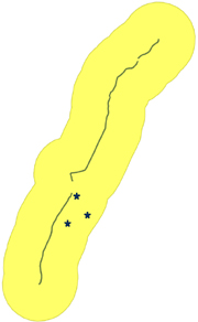
As you can see, not only is PostgreSQL/PostGIS a good analytical tool for doing simple number stats on spatial data, but it can also be used to render portions of an area of interest on a map. It can also be used to generate derivative geometries such as buffers that help highlight results.
1.7. Summary
In this chapter, we’ve given you a small taste of a spatially enabled database and how it fits in a relational database system. We sowed the budding idea of how to model real-world objects in space with spatial constructs.
We championed PostgreSQL and its spatial companion PostGIS. We demonstrated how PostgreSQL and PostGIS can be used together to analyze spatial patterns in data. We hope we’ve convinced you that the PostgreSQL/PostGIS combination is one of the best choices (if not the best) for spatial analysis.
Some of the SQL examples we demonstrated were on an intermediate level. If you’re new to SQL or spatial databases, these examples may have seemed daunting. In the chapters that follow, we’ll explain the functions we used here and the SQL constructs in greater detail. For now, we hope that you focused on the general steps we took and the strategies that we chose.
Although spatial modeling is an integral part of any spatial analysis, we pointed out that there’s no right or wrong answer in modeling. Modeling is inherently a balance between simplicity and adequacy. You want to make your model as simple as possible to focus on the problem you’re trying to solve, but you must retain enough complexity to simulate the world you’re trying to model. Therein lies the challenge.
Before we can continue our journey, we must first analyze the different geometry types that PostGIS offers us and show you how to create these and when it’s appropriate to do so. We’ll explore geometries in greater detail in chapter 2.