
Appendix C. SQL primer
PostgreSQL supports almost the whole ANSI SQL-92, 1999 standard logic as well as many of the SQL:2003, SQL:2006, and some of the SQL:2008 constructs. In this appendix we’ll cover these as well as some PostgreSQL-specific SQL language extensions. Because we’re remaining fairly focused on standard functionality, the content in this appendix is applicable to other standards-compliant relational databases.
Information_schema
The information_schema is a catalog introduced in SQL-92 and enhanced in each subsequent version of the specs. Although it’s a standard, sadly most commercial and open source databases don’t completely support it. We know that the following common databases do: PostgreSQL (7.3+), MySQL 5+ (not sure about 4), and Microsoft SQL Server 2000+.
The most useful views in this schema are tables, columns, and views; they provide a catalog of all the tables, columns, and views in your database.
To get a list of all non-system tables in PostgreSQL, you can run the following query, which will work equally well in MySQL (except that in MySQL schema means “database” and there’s only one information_schema shared across all MySQL databases in a MySQL cluster). MS SQL Server behaves more like PostgreSQL in that each information_schema is unique to each database, except that in SQL Server the system views and tables aren’t queryable from the information_schema, whereas they are in PostgreSQL. The tables view in PostgreSQL will list only tables that you have access to:
SELECT table_schema, table_name, table_type
FROM information_schema.tables
WHERE table_schema NOT IN('pg_catalog', 'information_schema')
ORDER BY table_schema, table_name;
The columns view will give you a listing of all the columns in a particular table or set of tables. In the following example we list all the geometry columns found in a schema called hello.
Listing C.1. List all columns in hello schema
SELECT c.table_name, c.column_name, c.data_type, c.udt_name,
    c.ordinal_position AS ord_pos,
    c.character_maximum_length AS cmaxl ,
    c.column_default AS cdefault
FROM information_schema.columns AS c
WHERE table_schema = 'hello'
ORDER BY c.table_name, c.column_name;
The results of this query look something like table C.1.
Table C.1. Results of query in listing C.1
|
table_name |
column_name |
data_type |
udt_name |
ord_pos |
cmax cdefault |
|---|---|---|---|---|---|
| coastline | coastline_id | integer | int4 | 1 | nextval(’hello....) |
| coastline | coastline_name | character varying | varcha | 2 | 150 |
| coastline | line_geom | USER-DEFINED | geometry | 3 |
One important way that PostgreSQL is different from databases such as SQL Server and MySQL server that support the information schema is that it has an additional field called udt_name that denotes the PostgreSQL-specific data type. Because PostGIS geometry is an add-on module and not part of PostgreSQL, you’ll see the standard ANSI data_type listed as USER-DEFINED and the udt_name storing the fact that it’s a geometry.
This view provides numerous other fields, so we encourage you to explore it. We’ve listed here what we consider the most useful fields:
- table_name and column_name— These should be obvious.
- data_type— The ANSI standard data type name for this column.
- udt_name— The PostgreSQL-specific name. Except for user-defined types, you can use the data_type or the udt_name when creating these fields except in the case of series. Recall that we created coastline_id as a serial data type, and PostgreSQL behind the scenes created an integer column and a sequence object and set the default of this new column to the next value of the sequence object: nextval(‘hello.coastline_coastline_id_seq’::regclass).
- ordinal_position— This is the order in which the column appears in the table.
- character_maximum_length— With character fields, this tells you the maximum number of characters allowed for this field.
- column_default— The default value assigned to new records. This can be a constant or the result of a function.
The tables view lists both tables and views (virtual tables). The views view gives you the name and the view_definition for each view you have access to. The view_definition gives you the SQL that defines the view and is very useful for scripting the definitions. In PostgreSQL, you can see how the information_schema views are defined, though you may not be able to in other databases such as SQL Server, because the information_schema is excluded from this system view.
SELECT table_schema, table_name, view_definition,
is_updatable, is_insertable_into
FROM information_schema.views
WHERE table_schema = 'information_schema';
In these examples, we demonstrated the common metatables you’d find in the ANSI information_schema. We also demonstrated the most fundamental of SQL statements. In the next section, we’ll tear apart the anatomy of an SQL statement and describe what each part means.
Querying data with Structured Query Language
The cornerstone of every relational database is the declarative language called Structured Query Language (SQL). Although each relational database has a slightly different syntax, the fundamentals are pretty much the same across all relational DBMSes.
One of the most common things done with SQL is to query relational data. SQL of this nature is often referred to as Data Manipulation Language (DML) and consists of clauses specifically designed for this. The other side of DML is updating data with SQL, which we’ll cover in the next section.
SELECT, FROM, WHERE, and ORDER BY clauses
For accessing data, you use a SELECT statement, usually accompanied with a FROM and a WHERE clause. The SELECT part of the statement restricts the columns to return, the FROM clause determines where the data comes from, and the WHERE restricts the number of records to return.
When returning constants or simple calculations that come from nowhere, the FROM clause isn’t needed in PostgreSQL, SQL Server, or MySQL, whereas in databases such as Oracle and IBM DB2, you need to select FROM dual or sys.dual or some other dummy table.
Basic Select
A basic select looks something like this:
SELECT gid, item_name, the_geom
FROM feature_items
WHERE item_name LIKE 'Queens%';
Keep in mind that PostgreSQL is by default case sensitive, and if you want to do a non-case-sensitive search, you’d do the following or use the non-portable ILIKE PostgreSQL predicate:
SELECT gid, item_name, the_geom
FROM feature_items
WHERE upper(item_name) LIKE 'QUEENS%';
There’s no guaranteed order for results to be returned, but sometimes you care about order. The SQL ORDER BY clause satisfies this need for order.
Following is an example that lists all items starting with Lion and orders them by item_name.
SELECT DISTINCT item_name
FROM feature_items
WHERE upper(item_name) LIKE 'LION%'
ORDER BY upper(item_name);
For pre PostgreSQL 8.4, you should uppercase your ORDER BY field, but PostgreSQL 8.4 provides a new per-database collation feature that makes this not as necessary depending on the collation order you’ve designated for your database.
Within a SELECT statement you can use the term *, which means “select all the fields in the FROM tables.” There is also the variant sometable.* if you want to select all fields from only one table and not all fields from the other tables in your FROM. We highly recommend you stay away from this with production code. This is useful for seeing all the columns of the table when you don’t have the table structure in front of you, but it can be a real performance drain, especially with tables that hold geometries. The reason for that is that if you have a table with a column that’s unconstrained by size, such as a large text field or geometry field, you’ll be pulling all that data across the wire and pulling from disk even when you don’t care about the contents of that field.
Indexes
The WHERE clause often relies on an index to improve row selection. If you have a large number of distinct groupings, it’s useful to put an index on that field. For a few distinct groupings of records by a column, the index is more harmful than helpful, because the planner will ignore it and do a faster table scan, and updating will even incur a heavy performance penalty.
Aliasing
In the examples using the information_schema, we demonstrated the concept of aliasing. Aliasing is giving a table or a column a different name in your query than how it’s defined in the database. It’s indispensible when doing SELF JOINs (where you join the same table twice) and need to distinguish between the two, or where the two tables you have may have field names in common. The other use is to make your code easier to read and also reduce typing by shortening long table and field names.
Aliasing is done with a statement AS. For table aliases, AS is optional for most ANSI-SQL standard databases including PostgreSQL. For column aliases, AS is optional for most ANSI SQL databases and PostgreSQL 8.4+ but required for PostgreSQL 8.3 and below.
Although AS is an optional clause, we like to always put it in for clarity. To demonstrate, which is more understandable?
SELECT b.somefield a FROM sometable b;
or
SELECT b.somefield AS a FROM sometable AS b;
Using Subselects
The SQL language has built-in support for subselects. Much of the expressiveness and complexity of SQL consists of keeping subselects straight and knowing when and when not to use them. For PostgreSQL most valid SELECT ... clauses can be used as subselects, and when used in a FROM clause, they must be aliased. For some databases such as SQL Server, there are some minor limitations; for example, SQL Server doesn’t allow an ORDER BY in a subselect without a TOP clause.
A subselect statement is a full SELECT ... FROM ... statement that appears within another SQL statement. It can appear in the following locations of an overall SQL statement:
- UNION, INTERSECT, EXCEPT— You’ll learn about these shortly.
- In the FROM clause— Where you’d normally put a table name and where it acts like a virtual table. The subselect needs to have an alias name to define how it will be called in other parts of the query, and it can’t reference other FROM table fields as part of its definition. Some databases allow you to do this under certain conditions such as SQL Server’s 2005+ CROSS APPLY.
- In the definition of a calculated column— When used in this context, the subselect can return only one column and one row. This pretty much applies to all databases. PostgreSQL has a somewhat unique feature because of the way it implements rows. A row is a data type and as such can be used as the data type of a column. This allows you to get away with returning a multicolumn row as a column expression. Because this isn’t a feature you’ll commonly find in other databases and is of limited use, we won’t cover it in this appendix. You can, however, return multiple rows as an array if they contain only one column using ARRAY in PostgreSQL. This will return the column as an array of that type. We demonstrate this in various parts of the book. Again this is a feature that’s fairly unique to PostgreSQL but very handy for spatial queries.
- In the WHERE part of another SQL query— In clauses such as IN, NOT IN, and EXISTS.
- In a WITH clause— This is loosely defined as a subquery but is not strictly thought of that way. Note that the WITH clause is available only in PostgreSQL 8.4+. You’ll also find it in Oracle, SQL Server 2005+, IBM DB2, and Firebird. You won’t find it in MySQL.
A correlated subquery is a subquery that uses fields from the outer query (next level above the subquery) to define the subquery. Correlated subqueries are often used in column expressions and WHERE clauses. They are generally slower than non-correlated subqueries because they have to be calculated for each unique combination of fields and have a dependency on the outer query.
In the following listing are some examples of subselects in action. Don’t worry if you don’t completely comprehend them, because some require an understanding of topics that we’ll cover shortly.
Listing C.2. Subselects used in a table alias
SELECT s.state, r.cnt_residents, c.land_area
FROM states As s LEFT JOIN
    (SELECT state, COUNT(res_id) As cnt_residents
        FROM residents
        GROUP BY state) As r ON s.state = r.state
LEFT JOIN (SELECT state, SUM(ST_Area(the_geom)) As land_area
        FROM counties
        GROUP BY state) As c
    ON s.state = c.state;
This statement uses a subselect to define the derived table we define as r. This is the common use case. We’ll demonstrate the same statement in listing C.3 using the PostgreSQL 8.4 WITH clause. The WITH clause, sometimes referred to as a Common Table Expression (CTE), is an advanced ANSI-SQL feature that you’ll find in SQL Server, IBM DB2, Oracle, and Firebird, to name a few.
Listing C.3. Same statement written using the WITH clause
WITH
     r AS (
         SELECT state, COUNT(res_id) As cnt_residents
            FROM residents
         GROUP BY state),
     c AS (
        SELECT state, SUM(ST_Area(the_geom)) As land_area
            FROM counties
        GROUP BY state)
SELECT s.state, r.cnt_residents, c.land_area
FROM states As s LEFT JOIN
    r ON s.state = r.state
LEFT JOIN c
    ON s.state = c.state;
In the next example, we demonstrate how to write the same query using a correlated subquery.
Listing C.4. Same statement written using a correlated subquery
SELECT s.state,
    (SELECT COUNT(res_id)
        FROM residents
        WHERE residents.state = s.state) As cnt_residents
, (SELECT SUM(ST_Area(the_geom))
    FROM counties
     WHERE counties.state = s.state) AS land_area
FROM states As s ;
Although you can use any of these to get the same result, the strategies used by the planner are very different, and depending on what you’re doing, one can be much faster than the other. With large numbers of returned rows, you should avoid the correlated subquery approach, but in certain cases it can be necessary to use a correlated subquery, for example, to prevent duplication of count.
JOINs
PostgreSQL supports all the standard JOINs and sets defined in the ANSI SQL Standards.
A JOIN is a clause that relates two tables usually by a primary and a foreign key, although the join condition can be arbitrary. In a spatial database you’ll find that the JOIN is often based on a proximity condition rather than on keys. The clauses LEFT JOIN, INNER JOIN, CROSS JOIN, RIGHT JOIN, FULL JOIN, and NATURAL JOIN exist in the ANSI SQL specifications. PostgreSQL supports all of these. SQL Server supports them as well. MySQL lacks FULL JOIN support. Oracle does support these, but it also has its own proprietary syntax (WHERE *= etc.) that is non-standard and is still often used today by long-time Oracle users.
Left Join
The LEFT JOIN returns all records from the first table (M) and only records in the second table (N) that match records in table (M). The maximum number of records returned by a LEFT JOIN is m*n rows, where m is the number of rows in M and n is the number of rows in N. The number of columns is the number of columns selected from M plus the number of columns selected from N.
Generally speaking, if your M table has a primary key that’s the joining field, you can expect the minimum number of rows returned to be m and the maximum to be m + mxn – n.
NULL placeholders are put in N table’s columns where there’s no match in the M table. You can see a diagram of a LEFT JOIN in figure C.1.
Figure C.1. Diagram of a LEFT JOIN. The darkened region represents the portion of records returned by a LEFT JOIN. The x stands for multiplication and the + is additive. The first circle is M and the second circle is N.

Following are a couple of examples of a LEFT JOIN:
SELECT c.city_name, a.airport_code,a.airport_name, a.runlength
FROM city As c
    LEFT JOIN airports As a ON a.city_code = c.city_code;
This query will list both cities that have airports and cities that don’t have airports based on the city_code. We assume city_code to be the city primary key with a foreign key in the airports table. If the LEFT JOIN were changed to an INNER JOIN, only cities with airports would be listed. With a LEFT JOIN, cities that have no airports will get a NULL placeholder for the airport fields.
One trick commonly used with LEFT JOINs is to return only unmatched rows by taking advantage of the fact that a LEFT JOIN will return NULL placeholders where there’s no match. When using this, make sure the field you’re joining with is guaranteed to be filled in when there are matches; otherwise, you’ll get spurious results. For example, a good candidate would be the primary key of a table. Here’s an example of such a trick:
SELECT c.city_name
FROM city As c
LEFT JOIN airports As ON a.city_code=c.city_code
WHERE a.airport_code IS NULL;
In this example code we’re returning all cities with no matching airports. We’re making the assumption here that the airport_code is never NULL in the airports table. If it were ever NULL, this wouldn’t work.
Inner Join
The INNER JOIN returns only records that are in both M and N tables, as shown in figure C.2. The maximum number of records you can expect from an inner join is (m x n). Generally speaking, if your M table has a primary key that’s the joining field, you can expect the maximum number of rows to be n. A classic example is customers joined with orders. If a customer has only five orders, the number of rows you’ll get back with that customer id and name is five.
Figure C.2. Diagram of an INNER JOIN. The darkened region represents the portion of records returned by the INNER JOIN. The x denotes that it’s multiplicative. The first circle is M and the second circle is N.

Following is an example of an INNER JOIN:
SELECT c.city_name, a.airport_code, a.airport_name, a.runlength
FROM city AS c
    INNER JOIN airports a ON a.city_code = c.city_code;
In this example we list only cities that have airports and only the airports in them. If we had a spatial database, we could do a JOIN using a spatial function such as ST_Intersects or ST_DWithin and could also find airports in proximity to a city or in a city region.
Right Join
The RIGHT JOIN returns all records in the N table and only records in the M table that match records in N, as shown in figure C.3. In practice, RIGHT JOIN is rarely used because a RIGHT can always be replaced with a LEFT, and most people find reading join clauses from left to right easier to comprehend. Its behavior is a mirror image of the LEFT JOIN, but flipping the table order in the clause.
Figure C.3. Diagram of a RIGHT JOIN. The darkened region represents the portion of records returned by a RIGHT JOIN. The x stands for multiplication and the + is additive. The first circle is M and the second circle is N.

Full Join
The FULL JOIN, shown in figure C.4, returns all records in M and N and puts in NULLs as placeholders in fields where there’s no matching data. There’s a lot of debate about the usefulness of this. In practice it’s rarely used, and some people are of the opinion that it should never be used because it can always be simulated with a UNION [ALL]. Although we rarely use it, in some cases, we find it clearer to use than a UNION [ALL].
Figure C.4. Diagram of a FULL JOIN. The darkened region represents the portion of records returned by a FULL JOIN. The x stands for multiplication and the + is additive. The first circle is M and the second circle is N.

The number of columns returned by a FULL JOIN is the same as for a LEFT, RIGHT, or INNER join; the minimum number of rows returned is max(m, n) and the maximum is (max(m,n) + mxn – min(m,n)).
While in theory it’s possible to do a FULL JOIN using spatial functions like ST_DWithin or ST_Intersects, in practice this isn’t currently supported, even as of PostgreSQL 9.0, PostGIS 1.5.
Cross Join
The CROSS JOIN is the cross product of two tables, where every record in the M table is joined with every record in the N table, as illustrated in figure C.5. The result of a CROSS JOIN without a WHERE clause is m x n rows. It’s sometimes referred to as a Cartesian product.
Figure C.5. Diagram of a CROSS JOIN. The darkened region represents the portion of records returned by the CROSS JOIN. The x stands for multiplication. The first circle is M and the second circle is N.

Here’s an example of a good use for a CROSS JOIN. The following calculates the total price of a product including state tax for each state:
SELECT p.product_name, s.state, p.base_price * (1 + s.tax) As total_price
FROM products AS p
CROSS JOIN state AS s;
It can also be written as
SELECT p.product_name, s.state, p.base_price * (1 + s.tax) As total_price
FROM products AS p, state AS s
Note that an INNER JOIN can be written with CROSS JOIN or (,) syntax and the WHERE part, but we prefer the more explicit INNER JOIN because it’s less prone to mistakes. When doing an INNER JOIN with CROSS JOIN syntax, you put the join fields in the WHERE clause. Primary keys and foreign keys are often put in the INNER JOIN ON clause, but in practice you can put any joining field in there. There’s no absolute rule about it. The distinction becomes important when doing LEFT JOINs, as you saw with the LEFT JOIN orphan trick.
Natural Join
A NATURAL JOIN is like an INNER JOIN without an ON clause. It’s supported by many ANSI-compliant databases. It automagically joins same named columns between tables; thus there’s no need for an ON clause.
We highly suggest you stay away from using this. It’s a lazy and dangerous way of doing joins that will come to bite you when you add new fields with the same names that are totally unrelated. We feel so strongly about not using this that we won’t even demonstrate its use. So when you see it in use, instead of thinking cool, just say no.
Chaining Joins
The other thing with JOINs is that you can chain them almost ad infinitum. You can also combine multiple JOIN types, but when joining different types, either make sure to have all your INNER JOINs first before the LEFTs or put parentheses around them to control their order. Here’s an example of JOIN chaining:
SELECT c.last_name, c.first_name, r.rental_id, p.amount, p.payment_date
FROM customer As C
   INNER JOIN rental As r ON C.customer_id = r.customer_id
   LEFT JOIN payment As p
   ON (p.customer_id = r.customer_id AND p.rental_id = r.rental_id);
This example is from the PostgreSQL pagila database. The pagila database is a favorite for demonstrating new features of PostgreSQL. You can download it from http://pgfoundry.org/projects/dbsamples/. In the previous example we find all the customers who have had rentals and list the rental fields as well (note that the INNER JOIN kicks out all customers who haven’t made rentals). We then pull the payments they’ve made for each rental and have NULLs if no payment was made but still list the rentals.
Sets
A set looks like a JOIN and is often lumped in with joins. What distinguishes a set class of predicates from a JOIN is that it chains together SQL statements that can normally stand by themselves to return a single dataset. The set class defines the kind of chaining behavior. Keep in mind when we talk about sets here, we’re not talking about the SET clause you’ll find in UPDATE statements.
SQL clauses we consider as sets are UNION [ALL], INTERSECT, and EXCEPT. PostgreSQL supports all three, though many databases support only the UNION [ALL].
One other distinguishing thing about sets is that the number of columns in each SELECT has to be the same, and the data types in each column should be the same too or autocast to the same data type in a non-ambiguous way.
One thing that confuses new spatial database users is the parallels between the two terminologies. In general SQL lingua franca you have UNION, INTERSECT, and EXCEPT, which talk about table rows, and when you add space to the mix, you have parallel terminology for geometries: ST_Union (which is like a UNION), ST_Collect (which is like a UNION ALL), ST_Intersection (which is like INTERSECT), and ST_Difference (which is like EXCEPT), which serve the same purpose for geometries.
Union and Union All
The most common type of set includes the UNION and UNION ALL sets, illustrated in figure C.6. Most relational databases have at least one of these and most have both. A UNION takes two SELECT statements and returns a DISTINCT set of these, which means no two records will be exactly the same. A UNION ALL, on the other hand, always returns n + m rows, where n is the number of rows in table N and m is the number of rows in table M.
Figure C.6. UNION ALL versus UNION. The thick box is M and the thinner box is N. The first UNION ALL shared regions are duplicated; in UNION only one of the shared regions is kept, resulting in a distinct set.

A union can have multiple chains each separated by a UNION ALL or UNION. The ORDER BY can appear only once and must be at the end of the chain. The ORDER BY is often denoted by numbers, where the number denotes the column number to order by.
A UNION is generally used to put together results from different tables. The following example will list all water features and land features greater than 500 units in area and all architecture monuments greater than 1000 dollars and will order results by item name.
Listing C.5. Combining water and land features
SELECT water_name As label_name, the_geom,
    ST_Area(the_geom) As feat_area
FROM water_features
WHERE ST_Area(the_geom) > 10000
UNION ALL
SELECT feat_name As label_name, the_geom,
    ST_Area(the_geom) As feat_area
FROM land_features
WHERE ST_Area(feat_geometry) > 500
UNION ALL
SELECT arch_name As label_name, the_geom,
    ST_Area(the_geom) As feat_area

FROM architecture
WHERE price > 1000
ORDER BY 1,3;
This example will pull data from three tables (water_features, land_features, and architecture) and return a single data set ordered by the name of the feature and then the area of the feature.
The plain UNION statement is often mistakenly used because it’s the default option when ALL isn’t specified. As stated, it does an implicit DISTINCT on the data set, which makes it slower than a UNION ALL. It also has another side effect of losing geometry records that have the same bounding boxes. We covered this in chapter 4. In short, be careful. In general, you want to use a UNION ALL except when deduping data where you want your datasets to be distinct.
Intersect
INTERSECT is used to join multiple queries, similar to UNION. It’s defined in the ANSI-SQL standard, but not all databases support it; for example, MySQL doesn’t support it, and neither does SQL Server 2000, although SQL Server 2005 and above do.
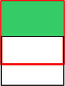
INTERSECT returns only the set of records that are common between the two result sets, as shown in figure C.7. It’s different from INNER JOIN in that it isn’t multiplicative and in that both queries must have the same number of columns. In the diagram in figure C.7, the green represents what’s returned by an SQL INTERSECT. Later we’ll look at a spatial intersection involving an intersection of geometries rather than an intersection of row spaces.
Figure C.7. INTER-SECT—the darkened region is the intersection of two data sets returned by an INTERSECT clause.

INTERSECT is rarely used. There are a couple of reasons for that:
- Many relational databases don’t support it.
- It tends to be slower than doing the same trick with an INNER JOIN. In PostgreSQL 8.4, the speed of INTERSECTs has been improved, though in prior versions it wasn’t that great.
- In some cases, it looks convoluted when you’re talking about the same table.
- In some cases it does make your code clearer, such as when you have two disparate tables or when you chain more than two queries. We demonstrate an example using INTERSECT and the equivalent query using INNER JOIN in the following listing.
Listing c.6. INTERSECT compared to INNER JOIN

![]() The query lists all water features greater than 500 square units that are also designated as protected areas inducted after
the year 2000.
The query lists all water features greater than 500 square units that are also designated as protected areas inducted after
the year 2000.
Note that if the feature_id field isn’t unique, the INNER JOIN runs the chance of multiplying records. To overcome that, you
may do a subselect, as shown in ![]() .
.
The next example demonstrates chaining intersect clauses:
SELECT r
     FROM generate_series(1,3) AS r
INTERSECT
SELECT n
    FROM generate_series(3,8) AS n
INTERSECT
SELECT s
    FROM generate_series(2,3) AS s
Keep in mind that you can mix and match with UNION and EXCEPT as well. The order of precedence is from top query down unless you have subselect parenthetical expressions.
Except
An EXCEPT chains queries together such that the final result contains only records in A that aren’t in B. The number of columns and type of columns in each chained query must be the same, similar to UNION and INTERSECT. The green section in figure C.8 represents the result of the final query.
Figure C.8. A demonstration of EXCEPT
EXCEPT is rarely used, but it does come in handy when chaining multiple clauses:
SELECT r
    FROM generate_series(1,3) AS r
EXCEPT
SELECT n
    FROM generate_series(3,8) AS n
INTERSECT
SELECT s
    FROM generate_series(2,3) AS s;
Using SQL aggregates
Aggregate functions roll a group of records into one record. In PostgreSQL the standard SUM, MAX, MIN, AVG, COUNT, and various statistical aggregates are available out of the box. PostGIS adds approximately nine to the list, of which ST_Collect, ST_Union, and ST_Extent are the most commonly used. We demonstrate an example of spatial aggregates in listing C.7 and several examples in this book. In this section we’ll focus on using aggregates. How you use aggregates is pretty much the same regardless whether they’re spatial or not.
Aggregates in SQL have generally the following parts:
- SELECT and FROM— This is where you select the fields and where you pull data from. You also include the aggregated functions in the select field list.
- SOMEAGRREGATE(DISTINCT somefield)— On rare occasions, you’ll use the DISTINCT clause within an aggregate function to denote that you use only a distinct set of values to aggregate. This is commonly done with the COUNT aggregate to count a unique name only once.
Note
With geometries, what is DISTINCTed is the bounding box, so different geometries with the same bounding box will get thrown out.
- WHERE— Non-aggregate filter; this gets applied before the HAVING part.
- HAVING— Similar to WHERE, except used when applying filtering on the already aggregated data.
- GROUP BY— All fields in the SELECT that are non-aggregated and function calls must appear here (pre PostgreSQL 9.1).
PostgreSQL 9.1 introduced the functional dependency feature, which means that if you’re already grouping by a primary key of a table, you can skip grouping by other fields in that table. This feature is defined in the ANSI SQL-99 Standard. It saves some typing as well as makes it easier to port some MySQL apps.
Fast Facts About Aggregate Functions
There are some important things you should keep in mind when working with aggregate functions. Some are standard across all relational databases, some are specific to PostgreSQL, and some are a consequence of the way PostGIS implements = for geometries.
- For most aggregate functions, NULLs are ignored. This is important to know because it allows you to do things such as COUNT(the_geom) as num_has_geoms, COUNT(neighborhood) as num_has_neighborhoods in the same SELECT statement.
- If you want to count all records, use a field that is never null to count, for example, COUNT(gid) or a constant such as COUNT(1). You can also use COUNT(*). Prior to PostgreSQL 8.1, the COUNT(*) function was really slow, so long-time PostgreSQL users tend to avoid that syntax out of habit.
- When grouping by geometries, which is very rare, it’s the bounding box of the geometry that’s actually grouped on (although the first geometry with that bounding box is used for output), so be very careful and avoid grouping by geometry if possible unless you have another field in the GROUP BY that’s distinct for each geometry, like the primary key of the table the geometry is coming from.
The following listing is an example that mixes aggregate SQL functions with spatial aggregates.
Listing C.7. Combining standard SQL and spatial aggregates
SELECT n.nei_name,
    SUM(ST_Length(roads.the_geom)) as total_road_length,
    ST_Extent(roads.the_geom) As total_extent,
     COUNT(DISTINCT roads.road_name) As count_of_roads
FROM neighborhoods As n
    INNER JOIN roads ON
        ST_Intersects(neighborhoods.the_geom, roads.the_geom)
WHERE n.city = 'Boston'
    GROUP BY n.nei_name
     HAVING ST_Area(ST_Extent(roads.the_geom)) > 1000;
The query for each neighborhood specifies the total length of road and the extent of roadway. It also includes a count of unique road names and counts only neighborhoods where the total area of the extent covered is greater than 1000 square units.
Window functions and window aggregates
PostgreSQL 8.4 introduced the ANSI-standard Window functions and aggregates, and PostgreSQL 9.0 improved on this feature by expanding the functionality of BETWEEN ROWS AND RANGE.
Window functionality allows you to do useful things such as sequentially number results by some sort of ranking, do running subtotals based on a subset of the full set using the concept of a window frame, and for PostGIS 1.4+ do running geometry ST_Union and ST_MakeLine calls, which are perhaps solutions in search of a problem but nevertheless intriguing.
A window frame defines a subset of data within a subquery using the term PARTITION BY, and then within that window, you can define orderings and sum results within the window to achieve rolling totals and counts. Microsoft SQL Server, Oracle, and IBM also support this feature, with Oracle’s feature set being the strongest and SQL Server’s being weaker than that of IBM DB2 or PostgreSQL. Check out our brief summary comparing these databases to get a sense of the differences: http://www.postgresonline.com/journal/index.php?/archives/122-Window-Functions-Comparison-Between-PostgreSQL-8.4,-SQL-Server-2008,-Oracle,-IBM-DB2.html.
PostgreSQL also supports named window frames that can be reused by name.
The following example uses the ROW_NUMBER() Window function to number streets sequentially that are within one kilometer of a police station, ordered by their proximity to the police station.
Listing C.8. Find roads within 1 km from each police station and number sequentially

In this listing we’re using ![]() the Window function called ROW_NUMBER() to number the results. The
the Window function called ROW_NUMBER() to number the results. The ![]() partition by clause forces numbering to restart for each unique parcel id (identified by pid) that uniquely identifies a
police station. The
partition by clause forces numbering to restart for each unique parcel id (identified by pid) that uniquely identifies a
police station. The ![]() ORDER BY defines the ordering. In this case we’re incrementing based on proximity to the police station. If two streets happen
to be at the same proximity, then one will be arbitrarily be n and the other n+1. Our ORDER BY includes road_name as a tie
breaker.
ORDER BY defines the ordering. In this case we’re incrementing based on proximity to the police station. If two streets happen
to be at the same proximity, then one will be arbitrarily be n and the other n+1. Our ORDER BY includes road_name as a tie
breaker.
In table C.2 we show a subset of our resulting table just for two police stations.
Table C.2. Results of window query in listing C.8
|
row_num |
pid |
road_name |
dist_km |
|---|---|---|---|
| 1 | 000010131 | Main Rd | 0.228687666823197 |
| 2 | 000010131 | Curvy St | 0.336867955509993 |
| 3 | 000010131 | Elephantine Rd | 0.959190964077745 |
| 1 | 000040128 | Elephantine Rd | 0.587036350160092 |
| 2 | 000040128 | Main Rd | 0.771250583026646 |
In the next section you’ll learn about another key component of SQL. SQL is good for querying data but also useful for updating and adding data as well.
UPDATE, INSERT, and DELETE
The other feature of DML is the ability to update, delete and insert data. An UPDATE, DELETE, and INSERT can combine the aforementioned predicates you learned for selecting data to do cross updates between tables or to formulate a virtual table (sub-query) to insert into a physical table. In the exercises that follow, we’ll demonstrate simple constructs as well as ones that are more complex.
Updates
We use the SQL UPDATE statement to update existing data. You can update individual records or a batch of records based on some WHERE condition.
Simple Update
A simple UPDATE will update data to a static value based on a where condition. Following is a simple example of this:
UPDATE things
SET status = 'active'
WHERE last_update_date > (CURRENT_TIMESTAMP - '30 day'::interval);
Update From Other Tables
A simple UPDATE is one of the more common UPDATE statements used. In certain cases, however, you’ll need to read data from a separate table based on some sort of related criteria. In this case you’ll need to utilize joins within your UPDATE statement. Here’s a simple example that updates the region code of a point data set if the point falls within the region:
UPDATE things
    SET region_code = r.region_code
    FROM regions As r
WHERE ST_Intersects(things.the_geom, r.the_geom);
Update With Subselects
A subselect, as you learned earlier, is like a virtual table. It can be used in UPDATE statements similar to the way you use regular tables. In a regular UPDATE statement even involving ones with table joins, you can’t update a table value to the aggregation of another table field. A way to get around this limitation of SQL is to use a subselect. Following is such an example that tallies the number of objects in a region:
UPDATE regions
    SET total_objects = ts.cnt
    FROM (SELECT t.region_code, COUNT(t.gid) As cnt
        FROM things AS t
        GROUP BY t.region_code) As ts
WHERE regions.region_code = ts.region_code;
If you’re updating all rows in a table, it’s often more efficient to build the table from scratch and use an INSERT statement rather than an UPDATE statement. The reason for this is that an UPDATE is really an INSERT and a DELETE. Because of the MVCC nature of PostgreSQL, PostgreSQL will remove the old row and replace it with the new row in the active heap. In the next section you’ll learn how to perform INSERTs.
INSERTs
Just like the UPDATE statement, you can have simple INSERTs that insert constants as well as more complex ones that read from other tables or aggregate data. We’ll demonstrate some of these constructs.
Simple Insert
The simple INSERT just inserts constants, and it comes in three basic forms.
The single-value constructor approach has been in existence in PostgreSQL since the 6.0 days and is pretty well supported across all relational databases. Here we insert a single point:
INSERT INTO points_of_interest(fe_name, the_geom)
    VALUES ('Highland Golf Club',
            ST_SetSRID(ST_Point(-70.063656, 42.037715), 4269));
The next most popular is the multirow value constructor syntax introduced in SQL-92, which we demonstrated often in this book. This syntax was introduced in PostgreSQL 8.2 and IBM DB2, has been supported for a long time in MySQL (we think since 3+) and was introduced in SQL Server 2008. As of this writing, Oracle has yet to support this useful construct. The multirow constructor is useful for adding more than a single row or as a faster way of creating a derived table with just constants. Following is such an example excerpted from earlier chapters. The multirow insert is similar to the single. It starts with the word VALUES, and then each row is enclosed in parentheses and separated with a comma.
Listing C.9. Multivalue row INSERT: two insert facilities
INSERT INTO hello.poi(poi_name, poi_geom)
VALUES ('Park',
        ST_GeomFromText('POLYGON ((86980 67760,
                 43975 71292, 43420 56700, 91400 35280,
      91680 72460, 89460 75500, 86980 67760))') ),
('Zoo',  ST_GeomFromText('POLYGON ((41715 67525, 61393 64101,
   91505 49252, 91400 35280, 41715 67525))') );
The last kind of simple INSERT is one that uses the SELECT clause, as shown in listing C.10. In the simplest example it doesn’t have a FROM. Some people prefer this syntax because it allows you to alias what the value is right next to the constant. It’s also a necessary syntax for the more complex kind of INSERT we’ll demonstrate in the next section. Note that this syntax is supported by PostgreSQL (all versions), MySQL, and SQL Server. To use it in something like Oracle or IBM DB2, you need to include a FROM clause, like FROM dual or sys.dual.
Listing C.10. Simple value INSERT using SELECT instead of VALUES
INSERT INTO points_of_interest(fe_name, the_geom)
    SELECT 'Highland Golf Club' AS fe_name,
        ST_SetSRID(ST_Point(-70.063656, 42.037715), 4269) As the_geom;


INSERT INTO hello.poi(poi_name, poi_geom)
SELECT 'Park' AS poi_name,
    ST_GeomFromText('POLYGON ((86980 67760,
                 43975 71292, 43420 56700, 91400 35280,
     91680 72460, 89460 75500, 86980 67760))') As poi_geom
UNION ALL
SELECT 'Zoo' As poi_name,
    ST_GeomFromText('POLYGON ((41715 67525, 61393 64101, 91505 49252,
   91400 35280, 41715 67525))')  As poi_geom;
This is the standard way of inserting multiple values into a table. It was the only way to do a multirow in pre PostgreSQL 8.2. This is also the only way to do it in SQL Server 2005 and below.
Advanced Insert
The advanced INSERT is not that advanced. You use this syntax to copy data from one table or query to another table. In the simplest case, you’re copying a filtered set of data from another table. It uses the SELECT syntax usually with a FROM and sometimes accompanying joins. Here we insert a subset of rows from one table to another:
INSERT INTO polygons_of_interest(fe_name, the_geom, interest_type)
SELECT pid, the_geom, 'less than 300 sqft' As interest_type
FROM parcels WHERE ST_Area(the_geom) < 300;
A slightly more advanced INSERT is one that joins several tables together. In this scenario the SELECT FROM is just a standard SQL SELECT statement with joins or one that consists of subselects. The following listing is a somewhat complex case: Given a table of polygon chain link edges, it constructs polygons and stuffs them into a new table of polygons.
Listing C.11. Construct polygons from line work and insert into polygon table
INSERT INTO polygons(polyid, the_geom)
SELECT polyid, ST_Multi(final.the_geom) As the_geom
FROM (SELECT pc.polyid,
   ST_BuildArea(ST_Collect(pc.the_geom)) As the_geom
    FROM
(SELECT p.right_poly as polyid, lw.the_geom
        FROM polychain p INNER JOIN linework lw ON
            lw.tlid = p.tlid
        WHERE (p.right_poly <> p.left_poly OR p.left_poly IS NULL)
    UNION ALL
    SELECT p.left_poly as polyid, lw.the_geom
        FROM polychain p INNER JOIN linework lw ON
            lw.tlid = p.tlid
        WHERE (p.right_poly <> p.left_poly OR p.right_poly IS NULL)
) As pc
GROUP BY poly.polyid) As final;
Select Into and Create Table As
Another form of the INSERT statement is what we commonly refer to as a bulk INSERT. In this kind of INSERT, not only are you inserting data, but you’re also creating the table to hold the data in a single statement. PostgreSQL supports two basic forms of this:
- One is the standard SELECT ... INTO, which a lot of relational databases support. We prefer this since because it’s more cross platform (will work on SQL Server as well as MySQL, for example).
- The other is a CREATE TABLE .. AS SELECT .., which isn’t as well supported by other relational databases.
In both cases any valid SELECT statement or WITH statement can be used. The following listing shows examples of the same statement written using SELECT INTO and CREATE TABLE AS.
Listing C.12. Example SELECT INTO and CREATE TABLE
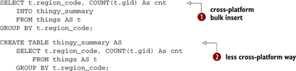
![]() This is the standard more cross-database-platform way of creating a table and inserting the data in one go.
This is the standard more cross-database-platform way of creating a table and inserting the data in one go. ![]() This is more of a PostgreSQL-specific way that’s a bit clearer in style but not as cross platform. If you need your code
to support multiple vendor databases, you’re better off with
This is more of a PostgreSQL-specific way that’s a bit clearer in style but not as cross platform. If you need your code
to support multiple vendor databases, you’re better off with ![]() .
.
DELETEs
DELETEs are the most limiting as far as joins go. When doing a DELETE you can’t join with any data so to define a subset of data to be deleted based on other information; you generally need to use an [NOT] EXISTS or [NOT] IN clause.
Simple Delete
A simple DELETE has no subselects but usually has a WHERE clause. All the data in a table is deleted and logged if you’re missing a WHERE clause. Following is an example of a standard DELETE:
DELETE FROM streets WHERE fe_name LIKE 'Mass%';
Truncate Table
In cases where you want to delete all the data in a table, you can use the much faster TRUNCATE TABLE statement. The TRUNCATE TABLE is considerably faster because it does much less transaction logging than a standard DELETE FROM, but it can be used only in tables that aren’t involved in foreign key relationships. Here’s an example of it at work:
TRUNCATE TABLE streets;
Advanced Delete
An advanced DELETE involves subselects in the WHERE clause. These are useful for cases where you need to delete all data in your current table that’s in the table you’re adding from or you need to delete duplicate records. The following example deletes duplicate records:
DELETE
FROM     sometable
WHERE    someuniquekey NOT IN
    (SELECT     MAX(dup.someuniquekey)
        FROM           sometable As dup
        GROUP BY     dup.dupcolumn1, dup.dupcolumn2, dup.dupcolum3);
Now that we’ve covered the basics of SQL in PostgreSQL, this concludes our SQL primer. In the next appendix, we’ll cover PostgreSQL-unique features such as its powerful language and stored function functionality, its extensive array support, and how security and backup are managed.