
Chapter 9. Performance tuning
When dealing with several tables at once—especially large ones—tuning queries, tables, and geometries becomes a major consideration. The way you express your queries is also important because the same logic expressed with two different SQL statements can have vastly different performance. The complexity of geometries, memory allocation, and even storage affect performance.
The query planner has many options to choose from, especially when joining tables. The planner can choose certain indexes over others, the order in which it navigates these indexes, and which navigation strategies (nested loops, bitmap scans, sequential scans, index scans, hash joins, and the like) it will use. All these play a role in the speed and efficiency of the queries.
It’s only partly true that SQL is a declarative language that allows you to state a request without worrying about the way it’s eventually implemented. The database planner may use one approach one day and for the same query use a different approach the next day because the distribution of data has changed. In practice, the way you state your question can greatly influence the way the planner answers it, and that answer has a great impact on speed. This is why all high-end databases provide “explain plans” or “show plans” to give you a glimpse of the planner’s strategy. SQL allows you only to ask questions and not define explicit steps, but you should still take care in how you ask your questions.
9.1. The query planner
All relational databases employ a query planner to digest the raw SQL statement prior to executing the query. The most important thing to keep in mind when writing a query is that the planner isn’t perfect and can optimize some SQL statements better than others. The query planner breaks down an SQL query into execution steps and decides which indexes, if any, and which navigation strategies will be used. It bases its plans on various heuristics and on its knowledge of the data distribution. It knows something that you often don’t know: how your data is distributed at any point in time. It won’t, however, relieve you of having to write efficient queries.
The spatial world of PostGIS offers some classic examples:
- One such example is asking for the top five closest objects, which we covered in chapter 5. (If you ask this, you force the PostgreSQL planner to do a table scan of all records and rank them all by distance and pick
the top five). Or you can ask for the top five closest within 10 miles. In the second case, the planner can use a spatial
index to throw out all objects that aren’t within 10 miles and then scan the remaining. You don’t care about the 10 miles
and don’t want to make that a requirement, but it makes the planner’s task simpler. An example of what the two different SQL
statements look like is shown here:
The fast way:
SELECT restaurant_name
FROM restaurants
WHERE ST_DWithin(ST_GeomFromText(...), restaurants.the_geom,10)
ORDER BY ST_Distance(ST_GeomFromText(...), restaurants.the_geom)
LIMIT 5; The slow but more obvious way:
SELECT restaurant_name
FROM restaurants
ORDER BY ST_Distance(ST_GeomFromText(...), restaurants.the_geom) LIMIT 5; - Another example is what we called the left-handed trick (or LEFT JOIN trick). In this case you want to know everything that doesn’t fit a particular criterion, but the straightforward way often leads to inefficient planner strategies. So instead, you ask to collect all objects that meet a criterion that’s capable of using an index as well as the ones that don’t and throw out the meeting criteria. Surprisingly, this happens to work pretty well for most relational databases, whereas the straightforward question isn’t as often converted to an efficient strategy.
The planner and indexes are two core facilities constantly under improvement in PostgreSQL. As such, it’s important to keep an eye on these enhancements, especially when upgrading. Although this is the case for PostgreSQL 8.3-9.0 and PostGIS 1.3-1.5, future versions may be smart enough to not require such a low-distance span to get the top five. For example, currently in the works is a KNN GIST feature that allows for deeper inspection of GIST indexes. This will make things like point in large polygon proximity queries much faster and will also reduce the need for specifying a spanning distance or allow you to specify a much larger distance without penalty. Some of this work you may see in operation in PostgreSQL 9.1 or 9.2 and PostGIS 2.0/2.1.
Also note that nearest neighbor (NN) queries are different from spatial database to spatial database. Oracle has some functions, such as SDO_NN, specifically for optimizing these queries. SQL Server 2011 (code-named Denali) has enhanced its spatial indexes to provide better NN logic with a simple STDistance(g1, g2) > x syntax. SQL Server indexes have always been based on a gridding model as opposed to the R-Tree approach that both PostGIS and Oracle use. Therefore, tricks for optimizing these kinds of queries aren’t as portable between the different platforms as other tasks.
We’ll delve into these and other planner topics, such as PostgreSQL settings, as we examine real case scenarios.
9.1.1. Planner statistics
The planner uses data statistics as well as various server configurations (allocated memory, shared buffers, seq costs, and the like) to make its decision.
Most relational databases use planner statistics as input to their planner cost strategies. Planner statistics are updated in PostgreSQL when you do a
vacuum analyze verbose sometable;
or during one of PostgreSQL’s automated vacuum runs if you have autovacuum enabled. Note that from PostgreSQL 8.3 and above autovacuum is enabled by default unless you explicitly disable it in your postgresql.conf file. In addition, from PostgreSQL 8.3 on, you can selectively set the frequency of vacuum runs or turn off automated vacuuming for certain tables if you want. Selectively controlling vacuum settings for problem tables is generally a better option than completely disabling autovacuum.
A vacuum analyze will both get rid of dead rows as well as update planner statistics for a table. For bulk inserts and updates, it’s best to do a vacuum analyze of the table after a large load rather than waiting for PostgreSQL’s vacuum run.
You can also do a plain
analyze sometable verbose;
if you want to update the statistics without getting rid of dead tuples and want to see progress of the analyze.
Planner statistics are a summary of the distinct values in a table and a simple histogram of the distribution of common values in a table. You can get a sense of what they look like by first updating the statistics with
vacuum analyze us.states;
and then running a query:
SELECT attname As colname, n_distinct,
   array_to_string(most_common_vals, E'
') AS common_vals,
   array_to_string(most_common_freqs, E'
') As dist_freq
FROM pg_stats
  WHERE schemaname = 'us' and tablename = 'states';
The result of this query is shown in table 9.1.
Table 9.1. Result of planner statistics query
|
colname |
n_distinct |
common_vals |
dist_freq |
|---|---|---|---|
| gid | -1 | ||
| state | -1 | -1 | |
| state_fips | -1 | ||
| order_adm | -0.962264 | 0 | 0.0566038 |
| month_adm | -0.226415 | December | 0.169811 |
| day_adm | 0 | ||
| year_adm | -0.660377 | 1788 | 0.150943 |
| the_geom | -1 |
Having -1 in the n_distinct column means that the values are more or less unique across the table in that column. A number less than 1 tells you the percentage of records that are unique. If you see a number greater than 1 in the n_distinct column, then that’s usually the exact number of distinct records found. The common_vals column lists the most commonly observed values. For example, month_adm tells us that December is the most common month, and because our n_distinct number is relatively high, about 70% of the records will fall in the common_vals section for that column. This is useful to the planner, because it can use this information to decide the order in which to navigate tables and apply indexes as well as plan the strategy. It can also guess whether a nested loop is more efficient than a hash by looking at the where and join conditions of a query and estimating the number of results from each table. In the next section we’ll look into the mind of the planner and investigate how it reasons about the queries it has to assess.
The planner analyzes a sample of the records when analyze is run. The number of records sampled is usually about 10% but varies depending on the size of the table and the default_statistics_target. Note that you can also set planner statistics separately for each column in a table if you want more or fewer records to be sampled. You do this using ALTER TABLE ALTER COLUMN somecolumn SET STATISTICS somevalue. We cover this in more detail in appendix D.
9.2. Using explain to diagnose problems
There are a few items you should look for when troubleshooting query performance:
- What indexes, if any, are being used?
- What is the order of function evaluation?
- In what order are the indexes being applied?
- What strategies are used, for example, nested loop, hash join, merge join, bitmap?
- What are the calculated versus the actual costs?
- How many rows are scanned?
In this section we’ll go over all those considerations and demonstrate how to infer them by looking at sample query plans. PostgreSQL, like most relational databases, allows you to view both actual and planned execution plans.
If you’re coming from another relational database such as MySQL, SQL Server, or Oracle, you’ll recognize the PostgreSQL explain plan as a parallel to the following:
MySQL—Same as PostgreSQL—EXPLAIN sql_goes_here
Oracle—EXPLAIN PLAN for sql_goes_here
SQL Server—Has both a graphical explain plan (built into Enterprise Manager, Studio, or Studio Express) similar to pgAdmin’s graphical explain as well as a text explain plan similar to the PostgreSQL raw explain. The graphical explain in SQL Server is much more popular than the following text explain option:
SET SHOWPLAN_ALL ON

GO

sql_goes_here
There are three levels of explain plans in PostgreSQL:
- EXPLAIN— This doesn’t try to run the query but provides the general approach that will be taken without extensive analysis.
- EXPLAIN ANALYZE— This runs the query but doesn’t return an answer. It generates the true plan and timings without returning results. As a result it tends to be much slower than a simple EXPLAIN and takes at least the amount of time needed to run the query (minus network effects of returning the data). In addition to the rows estimated it provides actual row counts and timings for each step. In 8.4+ it also provides the amount of memory used. Comparing the actual times against the estimated ones is a good way of telling if your planner statistics are out of date.
- EXPLAIN ANALYZE VERBOSE— This does an in-depth plan analysis, and for PostgreSQL 8.4+ it also includes more information such as columns being output.
EXPLAIN ANALYZE VERBOSE provides you with the columns being pulled in the query. This can alert you, when you using the evil SELECT *, how costly it is. EXPLAIN ANALYZE also displays memory utilization.
The following exercises use some of our pre-generated as well as our loaded data.
9.2.1. Text explain versus pgAdmin III graphical explain
There are two kinds of plan displays you can use in PostgreSQL: textual explain plans and graphical explain plans. Each caters to a different audience or a different state of mind. We enjoy using both, but generally we find the graphical explain easier to scan, more visually appealing, and as a rule of thumb a good place to focus our efforts. In this section we’ll experiment with both. There are many PostgreSQL tools that provide a graphical explain plan and a textual explain plan, all different in look, ability to print, and so on. For this study we’ll focus on the pgAdmin III graphical explain plan packaged with PostgreSQL and the native raw text explain plan output by PostgreSQL.
What is a Text Explain?
A text explain is the raw format of an explain output by the database. This is a common feature that can be found in most relational databases, but PostgreSQL’s explain tends to be richer in content than that of most databases. The text explain in PostgreSQL is presented as indented text to demonstrate the ordering of operations and the nesting of suboperations. You can output it using psql or pgAdmin III. For outputting nicely formatted text explains, the psql interface tends to be a bit better than pgAdmin III. There is also an online plan analyzer that outputs text plans nicely and highlights rows that you should be concerned about; it’s available at http://explain.depesz.com/help.
One of the latest changes in PostgreSQL 9.0 is the ability to output the text explain in XML, JSON, and YAML formats. This should provide more options for analyzing and viewing explain plans. We have an example of prettifying and making the JSON plan interactive using JQuery at http://www.postgresonline.com/journal/archives/174-pgexplain90formats_part2.html.
It generally provides more information than a graphical explain plan, which we’ll cover shortly, but tends to be harder to read and even sometimes provides too much information.
What is a Graphical Explain?
A graphical explain plan is a beautiful thing. It shows a diagram of how the planner has navigated the data, what functions it processed, and what strategies it has used—all this in bright and beautiful glowing icons and colors. The pgAdmin III graphical explain plan is quite attractive to look at. It has cute little icons for window aggs, hash joins, bitmap scans, and CTEs and provides tool tips as you mouse-over the diagram. In addition, the thickness of the lines gives a sense of the cost of a step. Thicker lines mean more costly steps. It’s similar in flavor to the Microsoft SQL Server show plan. In pgAdmin III 1.10 and above you can save the plan as an image.
In the next set of exercises we’ll look at some sample plans of queries and describe what each is telling us. We’ll look at each in its raw intimidating text explain form and its user-friendly cute pgAdmin III graphical presentation.
9.2.2. The plan without an index
We purposely didn’t index our tables so that we could demonstrate what a plan without an index looks like.
Example San Francisco Bridges Again
In this example we look at the simple intersects query from the last chapter. We’ll demonstrate the three text plans EXPLAIN, EXPLAIN ANALYZE, and EXPLAIN ANALYZE VERBOSE to see what further level of analysis each provides. We’ll then follow up with the graphical explain.
EXPLAIN SELECT c.city, b.bridge_nam
FROM sf.cities AS c INNER JOIN
  sf.bridges As b ON ST_Intersects(c.the_geom, b.the_geom);
The textual query plan of this explain is as follows:
QUERY PLAN
-----------------------------------------------------------------------
 Nested Loop  (cost=14.40..1185.55 rows=1 width=128)
   Join Filter: ((c.the_geom && b.the_geom) AND
           _st_intersects(c.the_geom, b.the_geom))
   ->  Seq Scan on cities c  (cost=0.00..21.15 rows=115 width=9809)
   ->  Materialize  (cost=14.40..18.40 rows=400 width=150)
         ->  Seq Scan on bridges b  (cost=0.00..14.00 rows=400 width=150)
The basic explain tells us the strategy the database would take to answer this question and also provides basic estimates of the cost of each step. It doesn’t actually run the query, so this explain is generally faster than the others—and for more intensive queries significantly faster. From the previous code you see the ST_Intersects function as two functions: an && operator that does a bounding box intersect check and the _st_intersects that does the more intensive intersect checking. You’ll only see this behavior with functions written in SQL because SQL functions are often inlined in queries and so are transparent to the planner. This allows the planner to reorder the function, even splitting it into two and evaluating the parts out of order. An inlined function is generally a good feature, but it can be bad too if it distracts the planner from more important analysis or encourages it to use an index where not using an index is more efficient.
In this next example, we repeat the same SQL but use EXPLAIN ANALYZE to inspect it:
EXPLAIN ANALYZE SELECT c.city, b.bridge_nam
FROM sf.cities AS c INNER JOIN
  sf.bridges As b ON ST_Intersects(c.the_geom, b.the_geom);
The result of the EXPLAIN ANALYZE looks like this:
QUERY PLAN
----------------------------------------------------------
 Nested Loop  (cost=14.40..1185.55 rows=1 width=128)
   (actual time=135.028..159.759 rows=8 loops=1)
   Join Filter: ((c.the_geom && b.the_geom)
     AND _st_intersects(c.the_geom, b.the_geom))
   ->  Seq Scan on cities c  (cost=0.00..21.15 rows=115 width=9809)
  (actual time=31.796..32.277 rows=115 loops=1)
   ->  Materialize  (cost=14.40..18.40 rows=400 width=150)
                    (actual time=0.148..0.150 rows=4 loops=115)
         ->  Seq Scan on bridges b
            (cost=0.00..14.00 rows=400 width=150)
            (actual time=16.930..16.937 rows=4 loops=1)
 Total runtime: 163.551 ms
You can see that EXPLAIN ANALYZE provides more information. In addition to the plan, it provides us with actual timing, total time, and the number of rows being traversed. You can see, for example, that the slowest part of our query is the nested loop. Nested loops tend to be the real bottlenecks, but in many cases they’re necessary. As a general rule of thumb, you want to minimize the number of rows that fall in a nested loop check.
In the next example we’ll look at the same query with verbose added:
EXPLAIN ANALYZE VERBOSE SELECT c.city, b.bridge_nam
FROM sf.cities AS c INNER JOIN
  sf.bridges As b ON ST_Intersects(c.the_geom, b.the_geom);
The result with VERBOSE is shown here:
QUERY PLAN
-------------------------------------------
 Nested Loop  (cost=14.40..1185.55 rows=1 width=128)
    (actual time=4.114..36.481 rows=8 loops=1)
   Output: c.city, b.bridge_nam
   Join Filter: ((c.the_geom && b.the_geom)
  AND _st_intersects(c.the_geom, b.the_geom))
   ->  Seq Scan on cities c
   (cost=0.00..21.15 rows=115 width=9809)
    (actual time=0.007..0.099 rows=115 loops=1)
         Output: c.gid, c.city, c.area__, c.length__, c.the_geom
   ->  Materialize  (cost=14.40..18.40 rows=400 width=150)
    (actual time=0.001..0.003 rows=4 loops=115)
         Output: b.bridge_nam, b.the_geom
         ->  Seq Scan on bridges b
  (cost=0.00..14.00 rows=400 width=150)
  (actual time=0.006..0.010 rows=4 loops=1)
               Output: b.bridge_nam, b.the_geom
 Total runtime: 40.118 ms
Here you see the output of the VERBOSE variant. The VERBOSE version tells us also what columns are being output. Also notice that the time this one takes is much lower than for our EXPLAIN ANALYZE. Because both an EXPLAIN ANALYZE and an EXPLAIN ANALYZE VERBOSE run the query, the database already knows how to plan this query and may have the plan cached and some portion of the function calls cached in short-term memory. It doesn’t always cache function answers, but if it decides to do so, the function is marked as immutable and the cost of caching is cheaper than recalculating the answer. Now we’ll take a look at the friendly sibling, the graphical explain.
To summon the graphical explain in pgAdmin III, you highlight the SQL statement in the query window and click the Explain Query icon; you could also check the Analyze option if you want a more in-depth tool tip with real analysis, as shown in figure 9.1. The graphical explain, however, can’t handle VERBOSE, so checking Verbose would force a plain-text explain.
Figure 9.1. Graphical explain controls

Our pretty sibling looks like figure 9.2.
Figure 9.2. Graphical explain analyze of our bridge and city intersects query
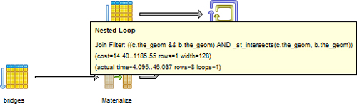
It’s a bit easier to see the order of operation with the graphical explain. The graphical explain always reads from left to right whereas with the text explain the time generally goes from bottom to top. Note that the nested loop is the last operation to happen. The other thing that’s nice about the graphical explain is the way it uses the thickness of the lines to denote the cost of a step. A thicker line, such as the one you see going to the nested loop in figure 9.2, means a more costly step. The tool tip feature is both good and bad. It’s good in the sense that it allows you to focus on one area; this is especially useful with complex queries. The downside is you can’t see all the detail at a glance as you can with the text version.
So you know now that we’re doing sequential scans on two tables and creating a work table (materialize means that we’re creating a temp table). For functions that are costly to calculate and are reused in the query and return few rows, you want the planner to materialize and may need to employ tricks to force that.
In the next section you’ll see what a plan with indexes looks like by rerunning the same query after adding spatial indexes and vacuum analyzing the sf.bridges and sf.cities tables.
9.3. Indexes and keys
There are many kinds of indexes you can use in PostgreSQL, and in many cases you’ll want to use more than one index. In almost all cases, you’ll want to use a spatial index. In some cases, you may want to use a B-tree or some other index access method as well.
The main families of indexes used in PostgreSQL are B-tree, GIST, and GIN; certain kinds of objects such as PostGIS are designed to take advantage of a certain index because of the way their data is structured. PostGIS, pgSphere, and Full Text Search objects can all use GIST indexes. Full Text Search can also use another index called a Generalized Inverted Tree (GIN) index, which is basically an R-tree (implemented with GIST) flipped upside down. Almost everything else works best with or can only use a B-tree index. Hash indexes are rarely used and are considered deprecated these days because they take longer to build and aren’t any faster than a B-tree or GIST, and for most applications that used to use them, they’re worse than a GIST index.
9.3.1. The plan with a spatial index scan
In the previous example you saw what our planner does without the help of indexes. In this listing, we’ll help the planner out a bit by adding spatial indexes to our tables. Observe how the planner reacts to this change of events.
Listing 9.1. Index, vacuum, explain

In this example we’ve indexed the tables ![]() and then
and then ![]() updated the statistics by vacuum analyzing. An analyze would have been sufficient, but as a general rule we vacuum because
vacuuming doesn’t add much more time if there are no dead tuples (no new updates) and reduces the records that need to be
scanned for future queries when there are dead tuples.
updated the statistics by vacuum analyzing. An analyze would have been sufficient, but as a general rule we vacuum because
vacuuming doesn’t add much more time if there are no dead tuples (no new updates) and reduces the records that need to be
scanned for future queries when there are dead tuples. ![]() Finally we do a full ANALYZE VERBOSE of our query. The associated graphical explain looks like this:
Finally we do a full ANALYZE VERBOSE of our query. The associated graphical explain looks like this:
QUERY PLAN
----------------------------------------------------------
 Nested Loop  (cost=0.00..22.17 rows=4 width=35)
   (actual time=0.609..30.487 rows=8 loops=1)
   Output: c.city, b.bridge_nam
   Join Filter: _st_intersects(c.the_geom, b.the_geom)
   ->  Seq Scan on bridges b  (cost=0.00..1.04 rows=4 width=401)
   (actual time=0.010..0.019 rows=4 loops=1)
         Output: b.gid, b.objectid, b.id, b.bridge_nam, b.the_geom
   ->  Index Scan using idx_sf_cities_the_geom on cities c
   (cost=0.00..5.27 rows=1 width=9809)
   (actual time=0.048..0.060 rows=3 loops=4)
         Output: c.gid, c.city, c.area__, c.length__, c.the_geom
         Index Cond: (c.the_geom && b.the_geom)
 Total runtime: 31.613 ms
What’s interesting about the query plan is that although we don’t have c.area and so on as part of the SELECT output, the planner is still dragging them along for the index and sequential scan. There’s a penalty with wide tables even if you aren’t selecting those columns, but the bigger penalty comes when you update even wider tables.
In figure 9.3 you see the graphical representation twice: one with the tool tip opened to the index and one opened on the nested loop.
Figure 9.3. Graphical explain after the addition of the index, first with the index tool tip and then with the nested loop tool tip

As you can see, the plan has changed simply by adding in some indexes. The main differences in this plan are as follows:
- The materialized table is gone.
- The index on sf cities is being used and an index scan is happening instead of a sequential scan.
- The ST_Intersects call has been split in order so the && part, which uses the spatial index scan, happens first, and the more costly _ST_Intersects call is the only one left in the nested loop. This is an important thing to look for in spatial queries, because sometimes this doesn’t happen even when you have an index. This is one of the most common reasons for slow performance when the index scan happens too late, sometimes even after the _ST_Intersects, or happens before a cheaper index scan.
- Most likely as a result of updated stats, our actual and estimated row numbers are closer. The closer the numbers the better, because closer numbers mean the planner’s estimates of the data distribution are more accurate.
- These tables are relatively small so our speed improvement isn’t significant after cache.
The planner employs a common programming tactic called short-circuiting. Short-circuiting occurs when a program processes only one part of a compound condition if processing the second part doesn’t change the answer. For example, if the first part of the logical condition “A and B” returns false, the planner knows it doesn’t have to evaluate the second part because the compound answer will always be false. This is a common behavior of relational databases and of many programming languages. But unlike many programming systems that implement short-circuiting, relational databases (PostgreSQL included) generally don’t check A and B in sequence. They first check the one they consider the cheapest. In the previous example with the index, you can see that the planner now considers the && cheaper than the _ST_Intersects, and so it processes that one first. Only after that will it process the _ST_Intersects for those records where geomA && geomB is true. For cost analysis, it looks at several things; with AND conditions, it often looks at the cost of a function and uses that to forecast how costly the operation is relative to others, but for OR compound conditions, function costs are ignored. Sometimes the cost of figuring out the cost is too expensive, so in those cases it simply processes the conditions in order. So even though the query planner may not process conditions in the order in which they’re stated, it’s still best for you to put the one you think is cheapest first.
This example also demonstrates the strengths and weaknesses of the plain-text plan versus the graphically enhanced plan. In the plain-text plan you can see at a glance how the ST_Intersects is broken up. In the graphical one, you need to mouse-over and click to see what’s happening.
9.3.2. Options for defining indexes
In addition to the various index types, you can also control which records are indexed with filter conditions or indexed on an expression instead of a column.
Partial Index
A partial index allows you to define criteria such as status=‘active’, and only data with that condition will be indexed. The main pros are as follows:
- It creates a smaller index so there’s less storage.
- The index is faster because it’s lighter and can better fit in memory.
- Sometimes it forces a more desirable strategy. For example, if your data is the same in 90% of the rows and different in only 10%, and you expect this to be the case for future data, it’s more efficient for the planner to scan only the index in the 10% and do a table scan for the other 90%. The planner has an easier time deciding whether to use an index.
These are the main cons:
- The where condition of the index has to be compatible with the queries it will be used in. This means the column your index filters by has to be used in a query for the planner to know whether the index scan is useful or not.
- Prepared statements can’t always use partial indexes. This bites you with parameterized prepared queries, queries of the form SELECT ... FROM sometable WHERE status = $1. The reason is that a plan with a parameter can’t assume anything about the value of that parameter; therefore it can’t determine whether to use the index. This is described in Hubert Lubaczewski’s Prepared Statements Gotcha at http://www.depesz.com/index.php/2008/05/10/prepared-statements-gotcha/.
- You can’t cluster on a partial index.
Here’s an example of a partial index:
CREATE INDEX idx_sometable_active_type
  ON sometable
  USING btree
  (type) WHERE active = true;
This situation presents itself where we normally query only active records for type and don’t care about type when pulling inactive records.
Compound Index
PostgreSQL, like most other relational databases, gives you the option of indexes composed of more than one table column or calculated columns but that use the same index access method. You can combine this with the aforementioned partial and the functional (aka expression) index, which we’ll discuss shortly.
A compound index is an index that’s based on more than one column. In PostgreSQL 8.1, the bitmap index plan strategy was introduced, which allowed using multiple indexes at the same time in a plan. The introduction of the bitmap index strategy made the compound index much less necessary, because you could combine several single-column indexes to achieve the same result. Still, in some cases, for example, if you always have the same set of columns in your WHERE or JOIN clause and in the same order, you might get better performance with a compound index, because a simple index scan is somewhat less expensive than a bitmap index scan strategy. Note that unlike some other databases such as SQL Server and MySQL that can take advantage of compound indexes (for some storage engines) to satisfy a query select (often called a covering index), PostgreSQL always fetches the rows from disk or cache because PostgreSQL indexes aren’t MVCC aware (they may contain indexes of dead records). There have been discussions to improve on this to implement true covering index behavior similar to what SQL Server offers. We’ll probably not see this enhancement until PostgreSQL 9.2. For a spatial index, it will always have to go to disk anyway because the GIST index is lossy (only indexes the bounding box). When people refer to covering index they generally mean an index that contains all the columns needed to satisfy a query, and there’s no need to retrieve extra data from disk.
Because most common data types don’t have operators for GIST access except for full-text search, you can’t include them in a GIST index, which makes combining them with spatial in a compound generally not possible.
Functional Index
The functional index, sometimes called an “expression index,” indexes a calculated value. It has two restrictions:
- The arguments to the function need to be fields in the same table, although the function can take as many columns or constants as arguments as it likes. You can’t go across tables or use aggregates and so on.
- The function must be marked immutable, which means that the same input always returns the same output and that no other tables are involved.
If you change the definition of an immutable function and this function is used in an index, you should reindex your table; otherwise, you’ll run into potentially bizarre results.
Functional indexes are pretty useful, especially for spatial queries. As mentioned earlier, we use ST_Transform functional indexes of the following form, which is a bit of a no-no:
CREATE INDEX idx_sometable_the_geom_2163 ON sometable USING
     gist(ST_Transform(the_geom,2163) );
For PostGIS 1.5, an even more useful functional index to use might be a geography index against a geometry column. This would give you the option of storing data in some UTM like geometry projection for display, advanced processing, and demonstration and yet be able to do long-range distance filters that would span multiple UTMs and still be able to use a spatial index. When you do this, you’d probably want to use a view to simplify your queries. The utility of this is debatable and probably doesn’t work well if you’re using third-party rendering tools where you can’t completely control the behavior of the generated query. We didn’t explore this approach and only throw it out as food for thought. Here’s an example (requires PostGIS 1.5 or above):
We can create a geography functional index by doing this:
CREATE INDEX idx_sometable_the_geom_geography
  ON sometable
  USING gist
  (geography(ST_Transform(the_geom,4326)));
Then we can use this index, by compartmentalizing our geography calculated field version in a view:
CREATE VIEW vwsometable AS
   SELECT *, geography(ST_Transform(the_geom,4326)) As geog
   FROM sometable As t;
Only when the record is pulled will the full geography output need to be calculated. For most cases, where we’re using geography as a filter in the WHERE clause, such as shown here, the indexed value will be used:
SELECT s1.field1 As s1_field1, s2.field1 As s2_field1
FROM vwsometable As s1 INNER JOIN
  vwsometable  AS s2
    ON(s1.gid <> s2.gid AND
ST_DWithin(s1.geog, s2.geog, 5000));
For this query, the spatial index might not be used if the costs on some functions are set too low. In that case, the planner has been given bad information and underestimates the cost of calculation versus the cost of reading from the index. We’ll revisit this when we talk about computing the cost of functions.
Other common uses for functional indexes in the spatial world are indexes on calculations with ST_Area or ST_Length, if you don’t want to store them physically, or putting a trigger on a table that’s filtered a lot where the filtering should be indexed. For geocoding, soundex is a common favorite. Following is an example of a soundex index and how it can be used.
The soundex function isn’t installed by default in PostgreSQL. To use it, you need to run the sharecontribfuzzystrmatch.sql file to load it. The fuzzy string match module contains other useful functions such as our favorite Levenshtein distance algorithm (which returns the Levenshtein distance between two strings—the least number of character edits you need to convert the first string to the second one).
In the next example we’ll demonstrate how to create a soundex index on a table and how to use it in a query. Keep in mind that you can use any function that’s marked immutable in a functional index.
CREATE INDEX idx_sf_stclients_streets_soundex
  ON sf.stclines_streets
  USING btree
  (soundex(street));
Then we update stats and clear dead tuples to make sure we get the best plan possible:
vacuum analyze sf.stclines_streets;
Finally we do our select using soundex:
SELECT DISTINCT street from sf.stclines_streets
WHERE soundex(street) = soundex('Devonshyer'),
Soundex is great for misspellings. The previous query would return “DEVONSHIRE” whether or not you have a soundex index in place. Note that because soundex doesn’t care about string casing, you can use it without changing your case to match your data. The previous query finishes in 16ms with the soundex index, and without the index it takes about 30ms. So in this case the index doesn’t add much because the speed is already pretty good. It does add a lot of speed if you’re dealing with a huge number of records.
Primary Keys, Unique Indexes, and Foreign Keys
There’s a lot of debate as to whether foreign keys are good as opposed to primary and unique keys, which we think most database specialists would consider a must have.
The planner uses information about primary key/unique index to know when to stop scanning for matches. This is especially important if you’re using inherited tables, because a primary key on the parent (though kind of meaningless), fools the planner into thinking it’s unique and it can stop checking once it hits a child with the requested key. There isn’t much difference between primary keys and a unique index except for the following:
- Only one primary key can exist per table, although you can have multiple unique indexes. Both primary keys and unique indexes can contain more than one column.
- Only primary keys can take part in foreign key relationships as the one side of a one-to-many relationship.
- A primary key can’t contain NULLs, but a unique key can and can even have many, but remember that NULLs are ignored when considering uniqueness.
Both have the side benefit of ensuring uniqueness (except in the case of NULLs) so will prevent duplication of data.
What about foreign keys that enforce referential integrity? A lot of people complain they impact performance. They impact performance only during updates/ inserts and in most cases negligibly unless you’re constantly updating the key fields. Although foreign keys in and of themselves don’t improve performance, they help in three indirect ways:
- They ensure you don’t have orphans, which generally means fewer records for the planner to scan through, wasting time, and in addition with CASCADING delete/update actions, they’re maintained by the database.
- They’re self-documenting; another database user can look at a foreign key relationship and know exactly how the two tables are supposed to be joined and that they’re related.
- Lots of third-party tools GUI query builders take advantage of them. So when an unsuspecting user drags and drops two tables in a query designer, the builder automatically joins the related fields.
Sometimes in a query, the planner refuses to use an index that you expected it to use. There are two main reasons for this:
- It can’t use the index because you didn’t set it up right. A common example of this is the B-tree index; how B-tree indexes behave changes from version to version. We’ll go more into detail about this in appendix D.
- The second reason is that a table scan is more efficient. If you think of an index as a thin table, scanning an index isn’t a completely free option. It costs additional reads, so the planner has to make the decision whether the effort of reading the index to determine the location of records to pull is less costly than scanning the raw data. For small tables or tables with many search hits, scanning the table is often faster.
Now that we’ve given you some fat to chew about deciding on indexes, we’ll explore how you can write your queries to change the planner’s behavior.
9.4. Common SQL patterns and how they affect performance
You know how to force a change of plan by adding in indexes. There are more complex join cases where you can control the plan by stating your query in different ways. In this section, we’ll demonstrate some of the common approaches for doing that.
Following are some general rules of thumb we’ll demonstrate in the accompanying exercises:
- JOINs are powerful and effective things in PostgreSQL and many relational databases; don’t shy away from them.
- Try to avoid having many subselects in the SELECT part of your query. If you find yourself doing this, you may be better off with a CASE statement.
- LEFT JOINs are great things, but especially with spatial joins, they’re a bit slower than INNER JOINs. If you use one, make sure you really need it.
We’ll start off by analyzing the many facets of a subselect statement and how where you position it affects speed and flexibility.
9.4.1. SELECT subselects
As mentioned in appendix C, a subselect can appear in the SELECT, WHERE, or FROM part of a query. For large numbers of rows to be returned, you’re much better off not using a subselect in the SELECT or WHERE clause, because it forces a query for each row, particularly if it’s a correlated subquery. For small numbers of records to return it varies, but it’s generally easier to read to put the query in the FROM clause. Sometimes you’re better off not using a subselect at all. If speed becomes problematic, you may have to test various ways of writing the same statement.
A correlated subquery is a query that can’t stand on its own because it uses fields from the outer query within its body. A correlated subquery always forces a query for each row, so it often results in slow queries.
The first exercise we’ll look at is the classic example of how many objects intersect with a reference object.
Exercise: How Many Streets Intersect Each City?
For this exercise we’ll ask this question with two vastly different queries. One is the naïve way in which people new to relational databases approach this problem, where they put the subselect in the SELECT. In some cases, counterintuitive to most database folk, this performs better or the same as the conventional JOIN approach. The second approach doesn’t use a subselect and uses the power of joins instead. Although the strategies of these are vastly different, the timings are pretty much the same for this data set.
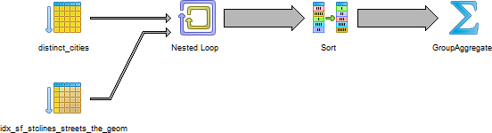
EXPLAIN ANALYZE SELECT c.city, (SELECT COUNT(*) AS cnt
  FROM sf.stclines_streets As s
  WHERE  ST_Intersects(c.the_geom, s.the_geom) ) As cnt
FROM sf.distinct_cities As c
ORDER BY c.city;
The output of the aforementioned analyze is as follows:
 Sort  (cost=825.49..825.73 rows=98 width=11484)
   (actual time=3663.059..3663.103 rows=98 loops=1)
   Sort Key: c.city
   Sort Method:  quicksort  Memory: 22kB
   ->  Seq Scan on distinct_cities c
 (cost=0.00..822.25 rows=98 width=11484)
   (actual time=1.464..3662.481 rows=98 loops=1)
         SubPlan 1
           ->  Aggregate  (cost=8.28..8.29 rows=1 width=0)
           (actual time=37.367..37.368 rows=1 loops=98)
                 ->  Index Scan using idx_sf_stclines_streets_the_geom
                 on stclines_streets s
   (cost=0.00..8.27 rows=1 width=0)
                 (actual time=12.567..37.226 rows=158 loops=98)
                       Index Cond: ($0 && the_geom)
                       Filter: _st_intersects($0, the_geom)
 Total runtime: 3664.534 ms
Now we’ll ask the same query but not using a subselect at all:
EXPLAIN ANALYZE SELECT c.city, COUNT(s.gid) AS cnt
FROM sf.distinct_cities As c
   LEFT JOIN sf.stclines_streets As s
       ON ( ST_Intersects(c.the_geom, s.the_geom) )
GROUP BY c.city
ORDER BY c.city;
Here’s the result:
GroupAggregate  (cost=649.24..651.20 rows=98 width=14)
 (actual time=3720.125..3737.232 rows=98 loops=1)
   ->  Sort  (cost=649.24..649.49 rows=98 width=14)
   (actual time=3720.102..3726.944 rows=15610 loops=1)
         Sort Key: c.city
         Sort Method:  quicksort  Memory: 1350kB
         ->  Nested Loop Left Join  (cost=0.00..646.00 rows=98 width=14)
         (actual time=1.228..3689.535 rows=15610 loops=1)
               Join Filter: _st_intersects(c.the_geom, s.the_geom)
               ->  Seq Scan on distinct_cities c
(cost=0.00..9.98 rows=98 width=11484)
(actual time=0.008..0.079 rows=98 loops=1)
               ->  Index Scan using
                    idx_sf_stclines_streets_the_geom on stclines_streets s
           (cost=0.00..6.48 rows=1 width=332)
      (actual time=0.018..0.682 rows=318 loops=98)
               Index Cond: (c.the_geom && s.the_geom)
 Total runtime: 3738.086 ms
Using a join is generally faster than the SELECT subselect, the more records your query outputs. When used in views, however, the planner is generally smart enough not to compute the column if it’s not asked for. In these cases, it’s better to put the subselect in the SELECT if you don’t need other fields from the subselect table and you know your subselect calculated column is rarely asked for. This is another reason to avoid the greedy SELECT * especially with views: You have no idea what complicated formula could be stuffed into a column.
Exercise: How Many Cities Have Streets, How Many Streets, and How- w Many are Longer Than 1000 Feet?
In this exercise, we’ll demonstrate the danger of subselects. When you see yourself having multiple subselects in your SELECT clause, ask yourself if they’re really necessary. Once again we’ll demonstrate this query using two different approaches, shown in the following listing. One is the naïve subselect way, and one is the JOIN way with CASE WHEN statements.
Listing 9.2. Subselects gone too far
EXPLAIN ANALYZE SELECT c.city, (SELECT COUNT(*) AS cnt
    FROM sf.stclines_streets As s
    WHERE  ST_Intersects(c.the_geom, s.the_geom) ) As cnt,
            (SELECT COUNT(*) AS cnt
    FROM sf.stclines_streets As s
    WHERE  ST_Intersects(c.the_geom, s.the_geom)
       AND ST_Length(s.the_geom) > 1000) As cnt_gt_1000
FROM sf.distinct_cities As c
  WHERE EXISTS(SELECT s.gid
    FROM sf.stclines_streets As s
    WHERE  ST_Intersects(c.the_geom, s.the_geom) )
ORDER BY c.city;
The result of this query are shown in the following listing.
Listing 9.3. Explain plan of subselect gone too far query
 Sort  (cost=662.59..662.60 rows=1 width=11484)
  (actual time=8553.707..8553.709 rows=4 loops=1)
    Sort Key: c.city
    Sort Method:  quicksort  Memory: 17kB
    ->  Nested Loop Semi Join  (cost=0.00..662.58 rows=1 width=11484)
    (actual time=16.260..8553.659 rows=4 loops=1)
          Join Filter: _st_intersects(c.the_geom, s.the_geom)
          ->  Seq Scan on distinct_cities c
            (cost=0.00..9.98 rows=98 width=11484)
            (actual time=0.005..0.078 rows=98 loops=1)
      ->  Index Scan using idx_sf_stclines_streets_the_geom on
      stclines_streets s
            (cost=0.00..6.48 rows=1 width=328)
            (actual time=0.018..0.166 rows=68 loops=98)
               Index Cond: (c.the_geom && s.the_geom)
         SubPlan 1
           ->  Aggregate  (cost=8.28..8.29 rows=1 width=0)
           (actual time=924.351..924.352 rows=1 loops=4)
                 ->  Index Scan using idx_sf_stclines_streets_the_geom
     on stclines_streets s  (cost=0.00..8.27 rows=1 width=0)
         (actual time=312.990..921.197 rows=3879 loops=4)
                        Index Cond: ($0 && the_geom)
                        Filter: _st_intersects($0, the_geom)
          SubPlan 2
           ->  Aggregate  (cost=8.28..8.29 rows=1 width=0)
           (actual time=909.088..909.089 rows=1 loops=4)
                 ->  Index Scan using idx_sf_stclines_streets_the_geom
      on stclines_streets s
                 (cost=0.00..8.28 rows=1 width=0)
                 (actual time=305.862..908.947 rows=124 loops=4)
                       Index Cond: ($0 && the_geom)
                       Filter: (_st_intersects($0, the_geom) AND
(st_length(the_geom) > 1000::double precision))
 Total runtime: 8555.406 ms
To the untrained eye, this query looks impressive because we’ve used complex constructs such as subselects, exists, and aggregates all in one query. In addition, the planner is making full use of index scans—and more than one at that. To the trained eye, this is a recipe for writing a slow and long-winded query. The graphical explain plan, shown in figure 9.4, looks particularly beautiful, I think.
Figure 9.4. EXPLAIN ANALYZE graphical plan for many subselect queries

Even though this does look convoluted, it has its place. It’s a slow strategy, but for building things like summary reports where your count columns are totally unrelated to each other except for the date ranges they represent, it’s not a bad way to go. It’s an expandable model for building query builders for end users where flexibility is more important than speed and where no penalty is paid if the column isn’t asked for.
PostgreSQL 9.0 introduced an enhancement to the planner that allows it to remove unnecessary joins. This feature will make queries using complex views that have lots of joins but the query selects few of these fields comparable in speed to (or faster than) the subselect approach.
The following is the same exercise solved with a CASE statement instead of subselect. A CASE statement is particularly useful for writing cross-tab reports where you use the same table over and over again and aggregate the values slightly differently.
EXPLAIN ANALYZE SELECT c.city, COUNT(s.gid) AS cnt,
    COUNT(CASE WHEN ST_Length(s.the_geom) > 1000 THEN 1 ELSE NULL END)
     As cnt_gt_1000
FROM sf.distinct_cities As c
   INNER JOIN sf.stclines_streets As s
       ON ( ST_Intersects(c.the_geom, s.the_geom) )
GROUP BY c.city
ORDER BY c.city;
The query plan of this looks like the following.
Listing 9.4. Query plan of count of streets and min length with no subselects
Sort  (cost=728.48..728.73 rows=98 width=342)
 (actual time=3751.973..3751.975 rows=4 loops=1)
   Sort Key: c.city
   Sort Method:  quicksort  Memory: 17kB
   ->  HashAggregate  (cost=723.28..725.24 rows=98 width=342)
   (actual time=3751.932..3751.936 rows=4 loops=1)
         ->  Nested Loop  (cost=0.00..646.00 rows=10304 width=342)
         (actual time=1.356..3700.814 rows=15516 loops=1)
               Join Filter: _st_intersects(c.the_geom, s.the_geom)
               ->  Seq Scan on distinct_cities c
               (cost=0.00..9.98 rows=98 width=11484)
               (actual time=0.005..0.074 rows=98 loops=1)
               ->  Index Scan using idx_sf_stclines_streets_the_geom on
                   stclines_streets s
               (cost=0.00..6.48 rows=1 width=332)
               (actual time=0.018..0.667 rows=318 loops=98)
                     Index Cond: (c.the_geom && s.the_geom)
 Total runtime: 3752.642 ms
As you can see, this query is not only shorter but also faster. Also observe that in this case we’re doing an INNER JOIN instead of a LEFT JOIN as we had done much earlier. This is because we care only about cities with streets. The results are shown in figure 9.5.
Figure 9.5. Cities with streets and count with min length using no subselects

As you can see from the diagram, the graphical explain plan is simpler but not as much fun to look at. It does have an exciting HashAggregate that combines both aggregates into a single call as a result of our CASE statement.
9.4.2. FROM subselects and basic common table expressions
A FROM subselect is a favorite of SQLers old and new. It allows you to compartmentalize all these complex calculations as columns into an alias that can be used elsewhere in your statement. In PostgreSQL 8.4 ANSI standard common table expressions, there’s a little twist added to the subselect that you know and love. The benefit of the common table expression is that it can reuse the same subselect in as many places as you want in your SQL statement without repeating its definition.
A couple of things about subselects used in FROM and in CTEs aren’t entirely obvious, even to those with extensive SQL backgrounds:
- Although you write a subselect in a FROM as if it’s a distinct entity, it’s often not. It often gets collapsed in (rewritten, if you will). It’s not always materialized, and the order of its processing isn’t even guaranteed.
- For PostgreSQL CTE incarnation, although the ANSI specs don’t require it, a CTE always seems to result in a materialization of the work table, although you can’t tell this from the plan because it shows a CTE strategy.
Be careful with CTEs because as stated in PostgreSQL 9.0 and below they always result in a materialization of the table expressions. Try to avoid table expressions within your overall CTE that return a lot of records unless you’ll be returning all those records in your final output. If your subquery returns many records and can be compartmentalized in the FROM clause, then you’d generally be better off with a sub-select in FROM rather than a CTE.
For small subselect tables with complex function calculations such as spatial function calculations, you generally want the subselect to be materialized, although for large data sets you don’t generally want subselects to be materialized. You can’t directly tell PostgreSQL this, but you can write your queries in such a fashion as to sway it in one direction or another. For PostgreSQL 8.4+ you’d write those expressions as CTE subexpressions to force a materialization. For prior versions of PostgreSQL you can throw in an OFFSET 0, which tricks the planner into thinking there’s a costly sort and makes it more likely that it will materialize or preprocess the costly subselect function calls. An example of using OFFSET follows. Note, however, that this isn’t guaranteed to cache. We recommend this kludge only if you’re observing significant performance issues. In those cases it doesn’t hurt to compare the timings to see which gives you better performance. For most queries it doesn’t make much of a difference, but for some, it can be fairly significant.
Here’s an example that uses OFFSET to encourage materialization:
SELECT a_gid, b_gid,
   dist/1000 As dist_km, dist As dist_m
FROM (SELECT a.gid As a_gid, b.gid As b_gid,
   ST_Distance(a.the_geom, b.the_geom) As dist
     FROM poly As a INNER JOIN poly As b
 ON (ST_Dwithin(a.the_geom, b.the_geom, 1000)  AND a.gid != b.gid)
    OFFSET 0
 ) As foo;
The example encourages caching of the distance calculation by making the subselect look more expensive. Because distance is a fairly costly calculation, if you’ll use it in multiple locations, you’ll prefer it to be materialized.
We describe examples of where this situation arises at http://www.postgresonline.com/journal/archives/127-PostgresQL-8.4-Common-Table-Expressions-CTE,-performance-improvement,-precalculated-functions-revisited.html; Andrew Dustan also demonstrates this at http://people.planetpostgresql.org/andrew/index.php?/archives/49-Well-use-the-old-offset-0-trick,-99..html.
Now that we’ve covered the use of subselects and CTES, we’ll explore Window functions and self-joins.
9.4.3. Window functions and self-joins
The Window function support introduced in PostgreSQL 8.4 is closely related to the practice of using self-joins. In prior versions of PostgreSQL, you could use a self-join to simulate the behavior of a window frame. In PostgreSQL 8.4+, there are still many cases where a self-join comes into play that still can’t be mimicked by a window in PostgreSQL. In PostgreSQL 9.0 the window functionality was enhanced, further minimizing the need of a self-join. For cases where you can use a window, and you aren’t concerned about backward compatibility with prior versions of PostgreSQL, then using a window frame approach is generally much more efficient and results in shorter code as well. The next listing demonstrates the same spatial query: one with a window and one with a self-join (the pre-PostgreSQL 8.4 way).
Listing 9.5. Rank number results using the self-join approach (pre-PostgreSQL 8.4)
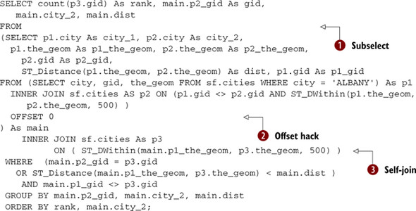
In this example, we employ lots of techniques in unison. We ![]() use a subselect to define a virtual worktable that will be used extensively to determine what cities are within 500 feet
of ALBANY.
use a subselect to define a virtual worktable that will be used extensively to determine what cities are within 500 feet
of ALBANY. ![]() We use the OFFSET hack described previously to encourage caching. Without the OFFSET our query takes 2 seconds, and with
the OFFSET the timing is reduced to 719 ms, a fairly significant improvement. This is because the costly distance check isn’t
recalculated.
We use the OFFSET hack described previously to encourage caching. Without the OFFSET our query takes 2 seconds, and with
the OFFSET the timing is reduced to 719 ms, a fairly significant improvement. This is because the costly distance check isn’t
recalculated. ![]() We do a self-join to collect and count all the cities that are closer to ALBANY than our reference p2 in main. Note the OR main.p2_gid = p3.gid; that way our RANK will count at least our reference geom even if there’s no closer object.
We do a self-join to collect and count all the cities that are closer to ALBANY than our reference p2 in main. Note the OR main.p2_gid = p3.gid; that way our RANK will count at least our reference geom even if there’s no closer object.
This more efficiently done with a Window statement, which is a feature supported in many enterprise relational databases and PostgreSQL 8.4+. The next example is the same query written using the RANK() Window function.
Listing 9.6. Using window frame to number results—PostgreSQL 8.4+

The equivalent window frame implementation using the RANK function is a bit cleaner looking and also runs much faster. This
runs in about 215 ms, and the larger the geometries the more significant the speed differences between the previous RANK hack
and the new one. In ![]() you see the declaration of WINDOW—WINDOW naming that doesn’t exist in all databases supporting windowing constructs. It allows
us to define our partition and order by frame and reuse it across the query instead of repeating it where we need it.
you see the declaration of WINDOW—WINDOW naming that doesn’t exist in all databases supporting windowing constructs. It allows
us to define our partition and order by frame and reuse it across the query instead of repeating it where we need it.
Now that we’ve covered the various ways you can write the same queries and how each one affects performance, we’ll examine what system changes you can make to improve performance.
9.5. System and function settings
Most system variables that affect plan strategy can be set at the server level, session level, or database level. To set them at the server level, edit the postgresql.conf file and restart or reload the PostgreSQL daemon service.
As of PostgreSQL 8.3, many of these can also be set at the function level.
Many of these settings can be set at the session level as well with
SET somevariable TO somevalue;
To set at the database level use
ALTER DATABASE somedatabase SET somevariable=somevalue;
Setting at the function level requires PostgreSQL 8.3+:
ALTER DATABASE somefunction(argtype1,argtype2,arg...) SET somevariable=somevalue;
To see the current value of a parameter use
show somevariable;
Now let’s look at some system variables that impact query performance.
9.5.1. Key system variables that affect plan strategy
In this section, we’ll cover the key system variables that most affect query speed and efficiency. For many of these, particularly the memory ones, there’s no specific right or wrong answer. A lot of the optimal settings depend on whether your server is dedicated to PostgreSQL work, the CPU and amount of motherboard RAM you have, and even whether your loads are more connection intensive versus more query intensive. Do you have more people hitting your database asking for simple queries, or is your database a workhorse dedicated to generating data feeds? Many of these settings you may want to set for specific queries and not across the board. We encourage you to do your own tests to determine which settings work best under what loads.
Constraint_Exclusion
In order to take advantage of inheritance partitioning effects, this variable should be set to On for PostgreSQL versions prior to 8.4 and set to Partition for PostgreSQL 8.4+. This can be set at the server or database level as well as the function or statement level. It’s generally best to set it at the server level so you don’t need to remember to do it for each database you create. The difference between the older On value and the new Partition value is that with Partition the planner doesn’t check for constraint exclusion conditions unless it’s looking at a table that has children. This saves a few planner cycles over the previous On. The On is still useful, however, with union queries.
Maintenance_Work_Mem
This variable is the amount of memory to allocate for indexing and vacuum analyze processes. When you’re doing lots of loads, you may want to temporarily set this to a higher number for a session and keep it lower at the server or database level:
SET maintenance_work_mem TO 512000;
Shared_Buffers
Shared_buffers is the amount of memory the database server uses for shared memory. This is defaulted to 32 MB, but you generally want this to be set a bit higher and be as much as 10% of available on-board RAM for a dedicated PostgreSQL box. This setting can only be set in the postgresql.conf file and requires a restart of the service after setting.
Work_Mem
Work_mem is the maximum memory used for sort operations and is set as the amount of memory in kb for each internal sort operation. If you have a lot of on-board RAM and do a lot of intensive geometry processing and have few users doing intensive things at the same time, this number should be fairly high. This is also a setting you can set conditionally at the function level or connection level, so keep it low for general careless users and high for specific functions.
ALTER DATABASE postgis_in_action SET work_mem=120000;
ALTER FUNCTION somefunction(text, text) SET work_mem=10000;
Enable (Various Plan Strategies)
The enable strategy options are listed here and all default to True/On. You never should change these settings at the server or database level, but you may find it useful to set them per session or at the function level if you want to discourage a certain plan strategy that’s causing query problems. It’s rare that you’d ever need to turn these off, and we personally have never had to. Some PostGIS users have experienced great performance improvements by fiddling with these settings on a case-by-case basis:
enable_bitmapscan, enable_hashagg, enable_hashjoin, enable_indexscan,
     enable_mergejoin, enable_nestloop, enable_seqscan, enable_sort,
     enable_tidscan
The enable_seqscan is one that’s useful to turn off because it forces the planner to use an index that it seemingly could use but refuses to. It’s a good way of knowing if the planner’s costs are wrong in some way or if a table scan is truly better for your particular case or your index is set up incorrectly so the planner can’t use it.
In some cases even settings that are turned off won’t be abided by. This is because the planner has no other choice of valid options. Setting them off will discourage the planner from using them but won’t guarantee it. These are
enable_sort, enable_seqscan, enable_nestloop
To play around with these, set them before you run a query. For example, turning off hashagg
set enable_hashagg = off;
and then rerunning our earlier CASE query that used a hashagg will change it to use a GroupAggregate, as shown in figure 9.6.
Figure 9.6. Cities’ streets and count with min length using no subselects after disabling the hashagg strategy
Disabling specific planner strategies is useful to do for certain critical queries where you know a certain planner strategy yields slower results. By compartmentalizing these queries in functions, you can control the strategies with function settings. Functions also have specific settings relevant only for functions. We’ll go over these in the next section.
9.5.2. Function-specific settings
Cost and row settings were introduced in PostgreSQL 8.3. The estimated cost and rows settings are available only to functions. They’re part of the definition of the function and not set separately like the other parameters.
The form is
CREATE OR REPLACE FUNCTION somefunction(arg1,arg2 ..)
  RETURNS type1 AS
....
  LANGUAGE 'c' IMMUTABLE STRICT
  COST 100 ROWS 2;
Cost
The Cost setting is a measure of how costly you think a function is. It’s mostly relevant to cost relative to other functions. Versions of PostGIS prior to 1.5 did not have these cost settings set, so under certain situations such as big geometries, functions such as ST_DWithin and ST_Intersects behaved badly and sometimes the more-costly process ran before the less-costly && operations. To fix this, you can set these costs in your install. You want to set the costs high on the non-public side of the functions _ST_DWithin, _ST_Intersects, _ST_Within, and other relationship functions. A cost of 100 for the aforementioned seems to work well in general, though no extensive benchmarking has been done on these functions to determine optimal settings.
Rows
This setting is relevant only for set-returning functions. It’s an estimate of the number of rows you expect the function to return.
Immutable, Stable, Volatile
As shown previously where you have IMMUTABLE, when writing a function, you can state what kind of behavior is expected of the output. If you don’t, then the function is assumed to be VOLATILE. These settings have both a speed as well as a behavior effect.
An immutable function is one whose output is constant over time given the same set of arguments. If a function is immutable, then the planner knows it can cache the result, and if it sees the same arguments passed in, it can reuse the cached output. Because caching generally improves speed, especially for pricey calculations, marking such functions as immutable is useful.
A stable function is one whose output is expected to be constant across the life of a query given the same inputs. These functions can generally be assumed to produce the same result, but they can’t be treated as immutable because they have external dependencies such as dependencies on other tables that could change. As a result they perform worse than an IMMUTABLE all else being equal but faster than a VOLATILE.
A volatile function is one that can give you a different output with each call even with the same inputs. Functions that depend on time or some other randomly changing factor or that change data fit into this category because they change state. If you mark a volatile function such as random() non-volatile, then it will run faster but not behave correctly because it will be returning the same value with each subsequent call.
Now that we’ve covered the various system settings you can employ to impact speed, we’ll take a closer look at the geometries themselves. Can you change a geometry so it’s still accurate enough for your needs, but the performance of applying spatial predicates and operations is improved?
9.6. Optimizing geometries
Generally speaking, spatial processes and checks on spatial relationships take longer with geometries with more vertices and holes, and they’re also either much slower or even impossible with invalid geometries. In this section we’ll go over some of the more common techniques to validate, optimize, and simplify your geometries.
9.6.1. Fixing invalid geometries
The main reasons to fix invalid geometries are:
- You can’t use GEOS relationship checks and many processing functions that rely on the intersection matrix with invalid geometries. Functions like ST_Intersects, ST_Equals, and so on return false or throw a topology error for certain kinds of invalidity regardless of the true nature of the intersection.
- The same holds true with Union, Intersection, and the powerful GEOS geometry process functions. Many won’t work with invalid geometries.
Most of the cases of invalid geometries are with polygons. The PostGIS wiki provides a good resource for fixing invalid geometries. A contrib function called cleanGeometry.sql does a fairly good job of this. See http://trac.osgeo.org/postgis/wiki/UsersWikiCleanPolygons.
In PostGIS 2.0, a function called ST_MakeValid was introduced that can be used to fix invalid polygons, multipolygons, multilinestrings, and linestrings.
In addition to making sure geometries are valid, you can improve performance by reducing the number of points in each geometry.
9.6.2. Reducing number of vertices with simplification
Reducing the number of vertices by simplifying the geometries has both speed improvement effects and accuracy tradeoffs.
Pros
There are two major advantages of simplifying geometries:
- It makes your geometries lighter in weight, which becomes increasingly important the more you zoom out on a map.
- It makes relationships, distance checks, and geometry processing faster because these functions are generally slower the more vertices you have. You can gain quite a performance increase by reducing an 80,000-point geometry to 8,000, for example.
Cons
These are the downside:
- Your geometries get less accurate. You’re trading precision for speed.
- You often lose colinearity—things that used to share edges no longer do, for example.
Simplification assumes a planar model, and so applying it to something designed to work with measurement around a spheroid will produce often unpredictable results. The best approach is to transform to a planar coordinate, preferably one that maintains measurement accuracy, and then retransform back to lon lat after the simplification process.
The following listing is a quick example of simplification, where we simplify our state boundaries and then compare performance before and after.
Listing 9.7. Simplified state versus non-simplified
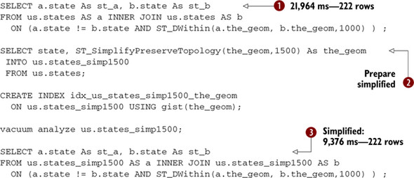
In listing 9.7 we run the usual ![]() distance check on our full-resolution data. This takes 21,964 ms and returns 222 rows. In
distance check on our full-resolution data. This takes 21,964 ms and returns 222 rows. In ![]() we create a new table called us.states_simp1500, which is our original data simplified with a tolerance of 1500 meters (basically
we treat points within 1500 meters as being equal). The units are in meters because our data is in National Atlas meters.
We then run the same query again
we create a new table called us.states_simp1500, which is our original data simplified with a tolerance of 1500 meters (basically
we treat points within 1500 meters as being equal). The units are in meters because our data is in National Atlas meters.
We then run the same query again ![]() against this new data-set. It completes in 9,376 ms and returns 222 rows. This was done using PostGIS 1.4.
against this new data-set. It completes in 9,376 ms and returns 222 rows. This was done using PostGIS 1.4.
In PostGIS 1.5, the ST_DWithin and ST_Distance functions were improved to better handle geometries with more vertices. As a result, the previous simplification isn’t as stark in PostGIS 1.5 as it is in prior versions.
In many cases you can get away with simplification on the fly and still achieve about the same performance benefit as with a stored simplification. The only thing you need to be careful of is not to lose the spatial index on the table in the process. To achieve this, we’ll create a new ST_DWithin function in the following listing that works against the simplified data but uses the original geometries for the index check operation so that the index is used.
Listing 9.8. Simplify on the fly and still use an index

In the example we ![]() create a new function that behaves like the built-in PostGIS ST_DWithin function, except that it applies a simplification
before doing the distance within check. Note that the index check && is applied to the original geometries to utilize the
spatial index on the tables. This new function takes in an additional argument compared with the standard PostGIS ST_DWithin:
the simplification tolerance. In
create a new function that behaves like the built-in PostGIS ST_DWithin function, except that it applies a simplification
before doing the distance within check. Note that the index check && is applied to the original geometries to utilize the
spatial index on the tables. This new function takes in an additional argument compared with the standard PostGIS ST_DWithin:
the simplification tolerance. In ![]() we don’t get quite as much performance improvement (14.7 seconds) as with our similar stored states_simp1500 (9.8 seconds).
However,
we don’t get quite as much performance improvement (14.7 seconds) as with our similar stored states_simp1500 (9.8 seconds).
However, ![]() by increasing the level of simplification, we get even faster performance (8.5 seconds). The trick is to find the maximum
simplification with acceptable loss in accuracy.
by increasing the level of simplification, we get even faster performance (8.5 seconds). The trick is to find the maximum
simplification with acceptable loss in accuracy.
In the next section, we’ll demonstrate another kind of simplification, and that’s removing unnecessarily small features from geometries.
9.6.3. Removing holes
In some situations you may not need holes. Holes generally add more processing time to things like distance checks and intersection. To remove them, you can employ something like the following code:
SELECT s.gid, s.city, ST_Collect(ST_MakePolygon(s.the_geom)) As the_geom
FROM (SELECT gid, city, ST_ExteriorRing((ST_Dump(the_geom)).geom) As the_geom
 FROM sf.cities )  As s
 GROUP BY gid, city;
We use ST_Dump to dump out the polygons from multipolygons. This is necessary because the ST_ExteriorRing function works only with polygons. We then convert the exterior ring to a polygon because the exterior ring is the linestring that forms the polygon. We use the common spatial design pattern of explode, process, collapse. The explode, process, collapse spatial design pattern is probably one of the most ubiquitous of all, especially for geometry massaging, similar to a baker preparing dough by kneading to remove the gas pockets.
You may not want to remove all holes, only the small ones that don’t add much visible or information quality to your geometry but do make other checks and processes slower. The next listing shows a simple method for removing holes of a particular size and is excerpted from the following article: http://www.spatialdbadvisor.com/postgis_tips_tricks/92/filtering-rings-in-polygon-postgis/.
Listing 9.9. Filter rings function and its application

To put this function to use with our San Francisco cities, we do this
SELECT s.city, filter_rings(the_geom, 51000) As newgeomnohole_lt5000
FROM sf.cities;
which returns each city with a new set of geometries, keeping only the holes that are greater than 51,000 square feet.
The next query will tell us which records have been changed by the previous query.
SELECT city, filter_rings(the_geom, 51000)) As newgeom
     FROM
    (SELECT city, the_geom,
        (SELECT SUM(ST_NumInteriorRings(geom))
     FROM ST_Dump(the_geom) ) As NumHoles
FROM sf.cities) As c
WHERE c.NumHoles > 0;
Note the use of ST_Dump in this query. It’s needed because the ST_NumInteriorRings returns only the number of holes in the first polygon, so if we’re dealing with a multi-polygon, we need to expand to polygons and then count the rings. You should encapsulate this into an SQL function if you use this construct often. Once again, this is the explode, process, collapse spatial design pattern at work.
9.6.4. Clustering
In this section, we’ll talk about two totally different optimization tricks that sound similar and even use the same terminology but mean different things. We’ll refer to the first as index clustering and the second as spatial clustering (bunching). The term bunching is more colloquial than industry standard. The index-clustering concept is one that’s fairly common and similarly named in other databases.
- Index clustering— By clustering we’re referring to the PostgreSQL concept of clustering on an index. This means you maintain the same number of rows, but you physically order your table by an index (in PostGIS usually the spatial one). This guarantees that your matches will be in close proximity to each other on the disk and easy to pick. Your index seeks will be faster because when reading the data pages each page will have more matches.
- Spatial clustering (bunching)— This is usually done with point geometries and reduces the number of rows. It’s done by taking a set of points, usually close to one another or related by similar attributes and aggregate by collecting them into multipoints. You can imagine in this case you’d be talking about 100,000 rows of multipoints versus 1,000,000 rows of points, which can be both a great space saver as well as a speed enhancer because you need fewer index checks.
Cluster On An Index
We’ve talked about this before in other chapters, but it’s worthwhile to revisit. First, how do you physically sort your table on an index?
ALTER TABLE sf.distinct_cities CLUSTER ON idx_sf_distinct_cities_the_geom;
CLUSTER verbose sf.distinct_cities;
Versions of PostgreSQL prior to 8.3 don’t allow clustering on a GIST (spatial) index that contains NULLs in the indexed field. Clustering is also most effective for readonly or rarely updated data.
Currently PostgreSQL doesn’t recluster a table, so to maintain order, you need to rerun the CLUSTER ... step. If you run CLUSTER without a table name, then all tables in the database that have been clustered will be reclustered.
Another important setting specific to tables is the FILLFACTOR. Those coming from SQL Server will recognize this term. It’s basically the target fullness of a database page. During cluster runs, the fill factor tries to be reestablished. For new inserts, the database will keep adding to a page until it’s that percentage full.
For static tables, you want the FILLFACTOR to be really high, like 99 or 100. A higher fill factor generally performs better in queries because the PostgreSQL can pull more data into memory with fewer pages. For data that you update frequently, you want this number to be the default (90) or less. This is because when you’re doing updates, PostgreSQL will try to maintain the order of existing records by inserting the newly updated row around the same location as where it was before. If there’s no space on the page, then it will need to create a new page, more likely ruining your cluster until you recluster.
FILLFACTOR can be set for both tables and indexes. Yes, indexes have pages too. To set the FILLFACTOR of a table you do something of the form
ALTER TABLE sf.bridges SET (FILLFACTOR=80);
Using Multipoints Instead of Points
For small geometries such as points that share more or less the same attributes, you may want to reduce the number of records by storing them clustered into proximity groups. One example is the location of trees where your proximity checks are just as good if you can talk about certain trees in a family. Intersects checks on these are often faster if you’re comparing fewer multipoints to multipoints versus more records. The following query clusters points together, grouping by some key features and proximity. For clustering, ST_SnapToGrid comes in quite handy.
Listing 9.10. Collecting points into multipoint bunches
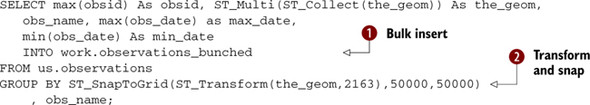
This example takes the observation points we created in WGS 84 lon lat and clusters them into 5000x5000 meter grids. ![]() We transform to National Atlas meters so that our snap-to-grid measurements will be in meters.
We transform to National Atlas meters so that our snap-to-grid measurements will be in meters. ![]() We then take the last ID as our new ID, the collected points that snap to the same grid and share the same name, use the
name, and store the min and max observation dates of our collected points. The new dataset has 8,163 records compared to our
original 27,316.
We then take the last ID as our new ID, the collected points that snap to the same grid and share the same name, use the
name, and store the min and max observation dates of our collected points. The new dataset has 8,163 records compared to our
original 27,316.
9.7. Summary
In this chapter we covered the various ways of improving the performance of spatial queries.
We discussed various approaches for writing spatial queries, how to troubleshoot query performance, how to optimize geometries, and what common settings in PostgreSQL can be changed to improve performance. Although many of these techniques focused on spatial queries, many can be applied to non-spatial queries as well.
PostGIS and PostgreSQL aren’t islands. They intermingle with various applications and software. The power of PostGIS can only be fully appreciated when you combine it with other tools to build applications or to view outputs. In the chapters that follow, we’ll take a closer look at how PostGIS interacts with other tools for viewing and building applications. You’ll learn not only how to view PostGIS output but also how to make attractive end-user applications that leverage its power.