Chapter 2. Geometry types

 

 

In the first chapter we gave you a brief taste of what PostGIS is and which basic geometries it supports. This chapter continues by explaining how PostGIS manages geometry data stored in the database. You’ll learn about those tables in all PostGIS-enabled databases that provide an inventory of the geometry table columns and of the available spatial reference systems. We then show you the definition and characteristics of points, linestrings, and polygons and how to work with them in a PostGIS-enabled database. After covering these single geometries, we move on to geometries that are made up of collections of single geometries: multipoints, multi-linestrings, multipolygons, and geometrycollections. We then demonstrate creating the less-commonly used curved geometries and 3D geometries and outline the issues to consider when using these less-common geometry types.

2.1. Geometry columns in PostGIS

PostGIS extends PostgreSQL by introducing a data type called geometry. Most of the functions that come packaged with PostGIS work with the core set of geometry types (points, linestrings, polygons, and their multi counterparts), some are specific to linestrings such as the linear referencing functions, some ignore the third and fourth coordinates, and some reject curved geometries or don’t work well with geometrycollections. For all intents and purposes, you can treat geometry on a par with other PostgreSQL data types such as dates, numbers, and text.

 

 

2.1.1. The geometry_columns table

PostGIS uses a table named geometry_columns to store metadata associated with the geometry columns in the database. The installation of PostGIS automatically creates this table. The geometry_columns table provides housekeeping information about geometry columns in the database and is commonly used by third-party tools to gather a list of geometry layers in the database. All other OGC-compliant spatial databases have a table with a similar or the same name, because this table is defined in the OGC Simple Features for SQL (SF SQL) specs.

 

 

As of PostGIS 1.4, the geometry_columns table is made up of seven columns. Four of these—f_table_catalog, f_table_schema, f_table_name, and f_geometry_column—are used to store the name of the database (also known as the catalog), table schema, table name, and geometry column name. The three final columns merit more discussion: coord_dimension, SRID, and type.

Coord_Dimension

This is the coordinate dimension of the geometry column; permissible values are 2, 3, and 4. Yes, PostGIS supports up to four dimensions. The fourth dimension is non-spatial and often referred to as the M coordinate (the M stands for “measure”). All of the geometry manipulation features supported by PostGIS treat the fourth dimension as an extra attribute of a point in the geometry rather than as another spatial dimension. The fourth dimension can be a temporal dimension, but you could use it as an index for anything. We’ll talk more about this M coordinate when we get to points.

 

 

SRID

SRID stands for spatial reference identifier and is an integer that relates back to the primary key of the metatable spatial_ref_sys. PostGIS uses this table to catalog all the spatial reference systems available to the database. The spatial_ref_sys metatable contains the name of the spatial reference system, the parameters needed to reproject to another system, and by which authority the system has been defined.

 

 

Keep in mind that using a different SRID doesn’t change the fact that the coordinate system underlying PostGIS is rectangular Cartesian. This fact comes to prominence when we start to deal with geographical features where the curvature of the earth comes into play. Suppose we’re trying to measure the distance between two points that represent New York and Los Angeles using the PostGIS function ST_Distance(). Because PostGIS is based on a regular X-Y coordinate system, ST_Distance() will return the distance calculated using the Pythagorean theorem, not the great circle distance that you might expect. Even if we were to use spherical coordinates like latitudes and longitudes to map our features, the underlying calculations would treat these as planar. So to correctly calculate distances when your data is stored in spherical coordinates, you need to first transform to a planar-based spatial reference system or use the PostGIS geography data type introduced in PostGIS 1.5 to store lon lat data. The PostGIS geography data type has similar functions for inserting data and uses the same text representations, except that all coordinates are input and expressed in WGS 84 lon lat, measurements are always in units of meters/square meters, there are fewer functions, and it uses a view called geography_columns that’s always in sync with the tables. We’ll briefly cover this type in later chapters of this book.

The default SRID in pre-2.0 versions of PostGIS is -1 to represent the unknown SRID. Should you use the unknown SRID? The answer is no if you’re working with geographic data. If you know the spatial reference system of your data, and presumably you should if you have real geographic data, then you should explicitly specify it. If you’re using PostGIS for non-geographical purposes, such as modeling a localized architecture plan or demonstrating analytic geometry principles, it’s perfectly fine keeping your spatial reference as unknown.

 

 

You should also know that even though the spatial_ref_sys table has close to 4,000 entries, you’ll encounter plenty of instances where you have to add SRIDs not already in the table. You can also be adventurous and define your own custom spatial reference system and add it to the spatial_ref_sys table in any PostGIS database.

Type

This final column stores the geometry type as a varying character field—‘POINT’, ‘LINESTRING’, ‘POLYGON’, ‘MULTIPOLYGON’, and others. Another admissible data value here is ‘GEOMETRY’. ‘GEOMETRY’ defines a heterogeneous geometry column that can store any geometry type.

The final admonition we need to make about the geometry_columns table is that in pre-2.0 versions of PostGIS, it’s for informational purposes only. Manipulating the values in the table has no bearing whatsoever on the actual geometry column referred to by the table. For example, you can start by creating a column to be two-dimensional polygons. You can even insert a few rows of polygons into the new column, but should you return to the geometry_columns table and change the type from polygons to linestrings, your data won’t be revalidated. You’ll end up with metadata that’s out of sync with the actual data. For this reason, we recommend that you not edit the geometry_ columns table directly.

2.1.2. Interacting with the geometry_columns table

To avoid editing the records directly in the metadata tables, PostGIS offers five functions, which, when used, will handle any necessary interactions with the geometry_columns table:

• AddGeometryColumn— Adds a geometry column to a table and adds pertinent metadata to the geometry_columns table.
• DropGeometryTable— Deletes a table with a geometry column and also deletes all metadata about those geometry columns from the geometry_columns table.
• UpdateGeometrySRID— Should you stamp the wrong SRID on your table geometry column, this will fix all records and also update the geometry_columns meta-data table.
• Probe_Geometry_Columns— Has existed as long as PostGIS itself. It doesn’t destroy any information already in the geometry_columns table but only adds new valid entries and gives you some stats as to the number it adds. It doesn’t inspect views or tables that lack PostGIS constraints, so these kinds of tables and views can’t be added with probe_geometry_columns. Nor does it add missing constraints to tables.
• Populate_Geometry_Columns (introduced in PostGIS 1.4)—A bit more sophisticated than Probe_Geometry_Columns, it can be used to populate the geometry_columns metadata by inspecting table views and tables that lack geometry constraints. Note that if you call this without any arguments, it will delete all entries in geometry_columns and repopulate the table. Therefore, it may take longer to run than probe_geometry_columns. It also adds constraints to the tables it registers that lack SRID and type constraints.

Of the five functions described, only Populate_Geometry_Columns can be used to register views in the PostGIS geometry_columns table; however, you’re still free to register these and other tables manually by directly inserting into geometry_columns.

In all of our examples thus far, we used the AddGeometryColumn function to handle the creation of new geometry columns. Although you don’t need to use these functions for creating and maintaining the geometry columns, for pre-2.0 versions of PostGIS we highly recommend doing so because the functions will automatically register and maintain entries in the geometry_columns table. To demonstrate the advantage of using the maintenance functions, we’ll add a new geometry column of points to a table without using the AddGeometryColumn function. We’d need to go through the following steps to achieve the same result:

1. Use ALTER TABLE to create a new geometry column.
2. Add columnar constraint enforce_geotype_poi_geom to the table to ensure that only points are in the new column.
3. Add columnar constraint enforce_dims_poi_geom to the table to ensure only 2D geometries can be added to the column.
4. Add columnar constraint enforce_srid_poi_geom to the table to permit only SRID of -1.
5. Add an entry to the geometry_columns metatable noting that the new points column is a coordinate two-dimensional point layer with an unknown spatial reference system.

As you can see, using maintenance functions wherever possible greatly simplifies matters and reduces the likelihood of you forgetting a step. Now that you have a general idea of the supporting structures and maintenance functions PostGIS offers for geometries, we’ll explore what kinds of geometries PostGIS offers and how to create and add them to your database.

2.2. A panoply of geometries

PostGIS has a large variety of geometry types to choose from to help you model the real world or, for that matter, anything you can think of that involves shapes. In this section we’ll explore the geometric data types in PostGIS in detail. We’ll concentrate on the defining attributes of geometries, addressing questions such as “What makes a linestring a linestring?”

2.2.1. What’s a geometry?

In this book, we use the term geometry to both indicate the general idea of a geometric shape as used in GIS and to mean PostGIS geometric data types.

 

 

The best way to think about a geometry data type is to draw an analogy to numeric data types. In general, setting up a column in a data table and declaring that it will store numeric data isn’t precise enough. You have to go further and must make distinctions between floating point and fixed numbers. With fixed numbers, you can specify more attributes, like the number of places after the decimal point or whether a column will be signed or unsigned. Like numeric data types, a geometry data type is akin to a base data type from which you can derive more specific data types. At the root of geometry data types, you find points, linestrings, polygons, and curves, each with its own defining attributes.

Let’s delve into some concrete examples. We start by creating a table to store all the geometries to be shown:

CREATE TABLE my_geometries
(id serial NOT NULL PRIMARY KEY, name varchar(20));

For now, our table has nothing more than an autonumbered column (also known as a serial column in PostgreSQL parlance) and a column to store the name of the geometries. For the sake of brevity, we’re placing our new table in the default public schema. Without prefixing the table name, PostgreSQL follows the schema search path. Unless you’ve changed the search path order, the default search always starts with $user followed by the public schema. For production work involving databases with many tables, we strongly urge you to create your own schemas and to organize your tables around these schemas. Not only will you keep your tables in logical units, but you’ll find it easier when it comes time to upgrade PostGIS and for performing selective backups and restores.

2.2.2. Points

All PostGIS geometries are based on the Cartesian coordinate system. A point in 2D coordinate space is specified by its X and Y coordinates. In 3D space, a point has X, Y, and Z coordinates; in 2DM space, a point has X, Y, and M coordinates and a PointM geometry (a PostGIS geometry type in its own right to distinguish it from points in 3D space). In 3DM space, a point has an X, Y, Z, and M coordinates. (In OGC nomenclature, this is often represented as a distinct data type called Point MZ, but PostGIS prior to the 2.0 series represents this as data type POINT with four coordinates.)

 

 

The following call to the AddGeometryColumn function creates a new geometry point column, after which we add two pizza parlors and your home to our simple Cartesian world.

Listing 2.1. Adding points

SELECT AddGeometryColumn('public','my_geometries',
   'my_points',-1,'POINT',2);
INSERT INTO my_geometries (name,my_points)
VALUES ('Home',ST_GeomFromText('POINT(0 0)'));
INSERT INTO my_geometries (name,my_points)
VALUES ('Pizza 1',ST_GeomFromText('POINT(1 1)')) ;
INSERT INTO my_geometries (name,my_points)
VALUES ('Pizza 2',ST_GeomFromText('POINT(1 -1)'));

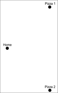
The code in listing 2.1 adds your home to the origin and two pizza parlors, one at (1,1) and one at (1,-1). Pull out a GIS desktop tool and you can see the three points, as shown in figure 2.1.

Figure 2.1. Three points created using the code in listing 2.1

2.2.3. Linestrings

Linestrings are defined by at least two distinct points. Like points, there are four dimensional variants of linestrings: linestring with points represented with X, Y coordinates; linestrings with points in X, Y, Z coordinates; linestrings with points in X, Y, M coordinates (also known as a LINESTRINGM); and finally linestrings with points represented in X, Y, Z, M coordinates. Let’s use the following listing to add a simple 2D linestring column with two rows.

Listing 2.2. Adding linestrings

SELECT AddGeometryColumn ('public','my_geometries',
  'my_linestrings',-1,'LINESTRING',2);
INSERT INTO my_geometries (name,my_linestrings)
VALUES ('Linestring Open',
  ST_GeomFromText('LINESTRING(0 0,1 1,1 -1)'));
INSERT INTO my_geometries (name,my_linestrings)
VALUES ('Linestring Closed',
  ST_GeomFromText('LINESTRING(0 0,1 1,1 -1, 0 0)'));

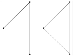
The first INSERT statement in listing 2.2 adds a linestring starting at the origin, going to (1,1) and terminating at (1,-1). This is an example of an open linestring where the starting and end points aren’t the same. The second INSERT statement adds a closed linestring. A closed linestring is a linestring where the starting and end points are the same. In modeling real-world geographic features, open linestrings predominate over closed linestrings. Rivers, streams, fault lines, and roads rarely start where they end. Closed linestrings, as you can see in figure 2.2, are the basis for constructing polygons.

Figure 2.2. Open and closed linestrings created using the code in listing 2.2. The points that make up the lines are shown as well.

The concept of simple and non-simple geometries comes into play when describing linestrings. A simple linestring can’t have self-intersections except at the starting and end points. A linestring that crosses itself isn’t simple. PostGIS provides a function, ST_IsSimple, that tests to see if a geometry is simple. The following query will return false:

SELECT ST_IsSimple(ST_GeomFromText('LINESTRING(2 0,0 0,1 1,1 -1)'));

The output of the SELECT is shown in figure 2.3.

Figure 2.3. A non-simple linestring tested for simplicity

Another important idea is that although a linestring is defined using a finite set of points, in reality you should think of it as being composed of an infinite number of points. This distinction becomes clear with questions relating to the closest point on a linestring to a polygon or other geometry. The closest point rarely coincides with any point used to define the linestring.

2.2.4. Polygons

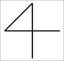
Now things get a little more interesting. We process from familiar geometries to form polygons. We start with a simple triangle: Take a closed linestring with at least three distinct points. This linestring takes the shape of a triangle, as shown in figure 2.4. All points enclosed by the linestring and the points on the linestring itself form the polygon. The closed linestring delineating the outer boundary of the polygon is called the ring of the polygon when used in this context; more specifically, it’s the exterior ring.

Figure 2.4. Triangle-shaped polygon

SELECT AddGeometryColumn('public','my_geometries',
  'my_polygons',-1,'POLYGON',2);
INSERT INTO my_geometries (name,my_polygons)
VALUES ('Triangle',
  ST_GeomFromText('POLYGON((0 0, 1 1, 1 -1, 0 0))'));

Many polygons used in geographical modeling consist of a single ring, but polygons can also have multiple rings. To be precise, a polygon can have one exterior ring and zero or more inner rings. Each interior ring creates a hole in the overall polygon, as shown in figure 2.5. This is why we need the seemingly redundant set of parentheses in the text representation of polygons. The well-known text (WKT) of a polygon is a set of closed line strings, with the first being the exterior ring and all subsequent designating the inner rings.

Figure 2.5. Polygon with interior rings (holes)

INSERT INTO my_geometries (name,my_polygons)
VALUES ('Square with 2 holes',
  ST_GeomFromText('POLYGON(
  (-0.25 -1.25,-0.25 1.25,2.5 1.25,2.5 -1.25,-0.25 -1.25),
  (2.25 0,1.25 1,1.25 -1,2.25 0),(1 -1,1 1,0 0,1 -1))'));

Always add the extra set of parentheses in the WKT, even if your polygon has just a single ring. Some tools may work with single-ringed polygons using only one set of parentheses without complaining, but not PostGIS.

In the real world, multiringed polygons play an important part in excluding bodies of water within geographical boundaries. For example, if we were planning a surface transit system in the greater Seattle area, we could start by outlining a big polygon bounded by Interstate 5 on the west and Interstate 405 on the east, as shown in figure 2.6. We could then start to pin down starting and terminal points of popular bus lines and let the computer choose the shortest path within the polygon. Soon enough, we’d realize that most of those popular routes are over water, Lake Washington to be specific. To have the computer pick routes correctly, our polygon of greater Seattle would need an inner ring outlining the shape of Lake Washington. This way, if we were to run a query asking for the shortest path between two points on the polygon and completely within the polygon, we wouldn’t end up with buses driving into the water.

Figure 2.6. We model the Seattle area as a polygon with two rings. Lake Washington fills up the hole. We’re also overlooking the existence of Mercer Island in the lake, which would make this a multipolygon.

With polygons we have the concept of validity. The rings of a valid polygon may only intersect at distinct points. What this means is that rings can’t overlap each other and that two rings can’t share a common boundary. A polygon whose inner rings partly lie outside its exterior ring is also invalid.

Figure 2.7 shows an example of a single polygon with self-intersections. (Visually, you can’t discern that it’s an invalid geometry because such a visual can be created with two valid polygons or one valid multipolygon that happens to be touching at a point.)

Figure 2.7. Example of a self-intersecting polygon with text representation of POLYGON((2 0,0 0,1 1,1 -1, 2 0))'). This is an example of an invalid polygon, but with the naked eye it’s impossible to see that it’s one invalid polygon and not one valid multipolygon or two valid polygons.

Not every invalid polygon lends itself to a pictorial representation. Degenerate polygons such as polygons with not enough points and polygons with non-closed rings are difficult to illustrate. Fortunately these polygons are difficult to generate in PostGIS and don’t serve any purpose in real-world modeling.

2.2.5. Collection geometries

To demonstrate the concept of collection geometries, we ask you to mentally picture the 50 states of the United States as polygons. Interior rings allow us to handle states with large bodies of water within their boundaries, such as Utah (the Great Salt Lake), Florida (Lake Okeechobee), and Minnesota with its 10,000-plus lakes. There’s at least one state that our polygon has trouble handling: Hawaii. Hawaii comes in at least five big pieces. We could conceivably model Hawaii as five separate polygons, but this complicates our storage. For example, if we wanted to create a table of states, we’d expect to have 50 rows. Breaking states into different polygons would call for storing a state using a state-polygon table, where each state could have up to hundreds of geometries depending on how fractured the state is. We’d lose the simplicity associated with one geometry per state.

To overcome this problem, PostGIS and the OGC standard offer geometry collections as data types in their own right. A collection of geometries is just that. It groups separate geometries that logically belong together. With the use of collections, each of our 50 states becomes a collection of polygons—a multipolygon.

 

 

In PostGIS each of the single geometry data types has a collection counterpart: multi-points, multilinestrings, multipolygons, and multicurves. In addition, PostGIS has a data type called geometrycollection. This data type can contain any kind of geometry as long as all geometries in the set have the same spatial reference system and the same coordinate dimension.

Multipoints

We start with multipoints, which are nothing more than collections of points. Figure 2.8 shows an example of a multipoint.

Figure 2.8. A single multipoint geometry—not three distinct points!

In order to represent a multipoint in WKT syntax, you’d use one of the following. If you have only X, Y coordinates for a multipoint, each comma-delimited value would have two coordinates:

MULTIPOINT(-1 1, 0 0, 2 3) (pictured)

For a 3DM multipoints, those having X, Y, Z, and M, you’d have four coordinates:

MULTIPOINT(-1 1 3 4, 0 0 1 2, 2 3 1 2)

For a regular 3D multipoint composed of (X, Y, Z), you’d have the following:

MULTIPOINT(-1 1 3, 0 0 1, 2 3 1)

For a multipoint where each point is composed of X, Y, M, you’d use MULTIPOINTM to distinguish it from an X, Y, Z multipoint:

MULTIPOINTM(-1 1 4, 0 0 2, 2 3 2)

 

 

We included MULTIPOINTM in our listings to remind you that all of the geometry collection data types have the M dimension type just like their single-geometry counterparts.

Multilinestrings

Of no surprise, a multilinestring is a collection of linestrings. Be mindful of the extra sets of parentheses in the WKT representation of a multilinestring that separate each individual linestring in the set. The following examples of multi-linestring are shown in figure 2.9.

Figure 2.9. Multilinest rings generated with WKT of inline examples

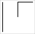
MULTILINESTRING((0 0,0 1,1 1),(-1 1,-1 -1))
MULTILINESTRING((0 0 1 1,0 1 1 2,1 1 1 3),(-1 1 1 1,-1 -1 1 2))
MULTILINESTRINGM((0 0 1,0 1 2,1 1 3),(-1 1 1,-1 -1 2))

Before moving on to multipolygons, let’s return to the concept of simplicity. In section 2.2.3, we tested a linestring for simplicity. Simplicity is relevant for all one-dimensional linestring type geometries. We consider multilinestrings simple if all constituent linestrings are simple and the collective set of linestrings doesn’t intersect each other at any point except boundary points. For example, if we create a multilinestring with two intersecting simple linestrings, the resultant multilinestring isn’t simple.

Multipolygons

Be careful! The WKT of multipolygons has even more parentheses than its singular counterpart. Because we use parentheses to represent each ring of a polygon, we’ll need another set of outer parentheses to represent multipolygons. With multipolygons, we highly recommend that you follow the PostGIS conventions and don’t omit any inner parentheses for single-ringed polygons. Following are some examples of multipolygons, the first of which is shown in figure 2.10:

Figure 2.10. Multipolygon generated with WKT of MULTIPOLYGON(((2.25 0,1.25 1,1.25 -1,2.25 0)),((1 -1,1 1,0 0,1 -1)))

MULTIPOLYGON(((2.25 0,1.25 1,1.25 -1,2.25 0)),
 ((1 -1,1 1,0 0,1 -1))) (pictured in figure 2.10)

MULTIPOLYGON(((2.25 0 1,1.25 1 1,1.25 -1 1,2.25 0 1)),
  ((1 -1 2,1 1 2,0 0 2,1 -1 2)) )

MULTIPOLYGON(((2.25 0 1 1,1.25 1 1 2,1.25 -1 1 1,2.25 0 1 1)),
  ((1 -1 2 1,1 1 2 2,0 0 2 3,1 -1 2 4))

MULTIPOLYGONM(((2.25 0 1,1.25 1 2,1.25 -1 1,2.25 0 1)),
  ((1 -1 1,1 1 2,0 0 3,1 -1 4)) )

Recall from the discussion on single polygons that a polygon is considered valid if all its rings don’t intersect or intersect only at distinct points. For a multipolygon to qualify as valid, it must pass two tests:

• Each constituent polygon must be valid in its own right.
• Constituent polygons can’t overlap. We’ll define overlap more rigorously in chapter 4, but even without that we think you get the picture: Once you lay down a polygon, subsequent polygons can’t be put on top and can share boundaries only at finite points.

Geometrycollection

Geometrycollection is a PostGIS data type that can contain heterogeneous geometries. Unlike multigeometries where the constituent geometries must be of the same type, the geometrycollection data type can include points, linestrings, polygons, and their collection counterparts. It can even contain other geometrycollections. In short, you can cram every geometry type known to PostGIS into a geometrycollection.

In listing 2.3, we present the WKT for geometrycollections, but instead of just showing you the WKTs, we include the SQL that generates them. We do this for a reason: In real-world applications, you should rarely define a data column as geometrycollection. Although having a heterogeneous collection is perfectly reasonable for storage purposes, most PostGIS functions won’t make any sense when used with these data types. For example, you can ask what the area is of a multipolygon, but you can’t ask what the area is of a geometrycollection that has linestrings and points in addition to polygons. Geometrycollections generally originate as a result of queries rather than as predefined columns. You should be prepared when you have to work with them, but avoid using them in your table design. The next listing shows you the result of union queries that generate geometrycollections.

Listing 2.3. Forming geometrycollections from constituent geometries

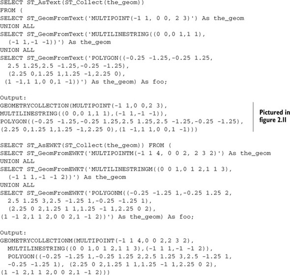
The output of the first geometrycollection of listing 2.3 is shown in figure 2.11. The output of the multim geometry would look the same, except that the M coordinate has no visual representation.

Figure 2.11. geometrycollection formed from code in listing

In this example we use ST_AsEWKT and ST_GeomFromEWKT to define our geometrycollection with an M coordinate. (The E stands for “extended.”) The reason for that is that the OGC-compliant functions of ST_AsText and ST_GeomFromText aren’t designed for anything above 2D, whereas ST_GeomFromEWKT and ST_AsEWKT are PostGIS constructs and can be used to display and create geometries of all dimensions. The other benefit of ST_AsEWKT over ST_AsText is that ST_AsEWKT will also return the spatial reference system if it’s known. The distinction between the two sets of functions may change in later versions of PostGIS.

Finally, a geometry collection is considered valid if all the geometries in the collection are valid. It’s invalid if any of the geometries in the collection are invalid.

2.2.6. Curved geometries

PostGIS 1.3 and above have rudimentary support for curved geometries. If you plan to use curved geometries, you definitely should use the latest PostGIS release. Curved geometries were introduced in the OGC SQL-MM Part 3 specs, and PostGIS has partial support of what’s defined in the specs.

Curved geometries aren’t as mature as other geometries and aren’t widely supported. Natural terrestrial features rarely manifest themselves as curved geometries. Manmade structures and boundaries do have curves, but for many modeling cases, these structures can be adequately approximated with lines. Aeronautical charts are full of them because the sweep of radar is circular. Dams, dikes, and breakwaters are other curved macro structures that come to mind. Some highways segments come close to being curves, but linestrings are often more appropriate in modeling them, certainly when processing speed is more important than accuracy. Because of lack of support, we offer the following caveats before you decide to go down the path of using curved geometries:

• Few third-party tools, either open source or commercial, support curved geometries.
• The advanced spatial library called GEOS that PostGIS uses for much of its functionality such as performing intersections, containments checks, and other spatial relation checks doesn’t support curved geometries. As a workaround, you can convert curved geometries to linestrings and regular polygons using the ST_CurveToLine function and then convert back with ST_LineToCurve. The downside of this method is the loss in speed and the inaccuracies introduced when interpolating arcs using linestrings.
• Many native PostGIS functions don’t support curved geometries. You can find a full list of functions that do support curved geometries in the PostGIS reference manual. Again, for cases where you need to use functions that don’t support curved geometries, you can use the ST_CurveToLine function, apply the function, and then apply the ST_LineToCurve function to convert back if needed.
• Curved geometries have not been supported for as long as the other geometries in PostGIS, so you’re more likely to run into bugs when working with them. More recent releases of PostGIS have cleaned up many of the bugs and have expanded the number of functions that support curved geometries.

Given all the drawbacks of curved geometries, you might be wondering why you’d ever want to use them. Here are a few reasons:

• You can represent a truly curved geometry with fewer points.
• More tools will inaugurate support for curved geometries. The Java2D graphical rendering library, Adobe Flex, Safe FME, and uDig 1.2 are the ones we know about that have or are working on curved geometry support usable by PostGIS.
• PostGIS is increasing support for curved geometries. The complete MM set for curved geometries should be available in PostGIS 2.0. You should also start enjoying complete support of intersections and relation checks in later versions.
• Curved geometries are particularly important when modeling manmade structures such as buildings and bridges, where true curved objects are commonly found.
• Even if you don’t store your data using curved geometry types, it’s often useful as an intermediary source to draw a quarter circle using curved geometry WKT and then convert to a regular polygon using the ST_CurveToLine function.

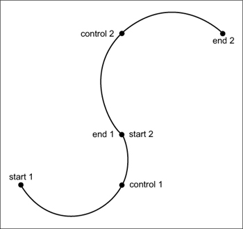
Let’s now take a closer look at the large variety of curved geometries. For simplicity, you can think of curved geometries in PostGIS as geometries with arcs. To build an arc, you must have exactly three distinct points. The first and last points denote the starting and end points of the arc, respectively. The point in the middle is called the control point because this point controls the degree of curvature of the arc.

Circularstring

A series of one or more arcs where the end point of one is the starting point of another makes up a geometry called a circularstring. Figure 2.12 is a diagram of a five-point circularstring.

Figure 2.12. A simple five-point circular string, the WKT CIRCULARSTRING (0 0,2 0, 2 1, 2 3, 4 3). The control points are POINT(2 0)and POINT(2 3).

 

 

The circularstring is the simplest of all curved geometries and contains only arcs. The following listing contains more examples of circularstrings and how you’d register them in the database.

Listing 2.4. Building circularstrings

SELECT AddGeometryColumn ('public','my_geometries',
  'my_circular_strings',-1,'CIRCULARSTRING',2);

INSERT INTO my_geometries(name,my_circular_strings)
VALUES ('Circle',
 ST_GeomFromText('CIRCULARSTRING(0 0,2 0, 2 2, 0 2, 0 0)')),
('Half Circle',
 ST_GeomFromText('CIRCULARSTRING(2.5 2.5,4.5 2.5, 4.5 4.5)')),
('Several Arcs',
 ST_GeomFromText('CIRCULARSTRING(5 5,6 6,4 8, 7 9, 9.5 9.5,
   11 12, 12 12)'));

The output of listing 2.4 is shown in figure 2.13.

Figure 2.13. Three circular strings generated from the code in listing 2.4

You’ll discover that not all rendering tools can handle curve geometries. In these instances, the ST_CurveToLine function comes in handy for approximating curved geometries with linestrings. As the following code and table 2.1 demonstrate, to achieve a reasonable degree of curvature, the linestring contains many segments:

Table 2.1. Observe how many more points the LINESTRING equivalent takes to approximate a curve.

Name	cnpoints	lnpoints
Circle	5	129
Half Circle	3	65
Several Arcs	7	113

SELECT name,ST_NPoints(my_circular_strings) As cnpoints,
     ST_NPoints(ST_CurveToLine(my_circular_strings)) As lnpoints
  FROM my_geometries
WHERE my_circular_strings IS NOT NULL;

Compoundcurves

Circularstrings and linestrings in series make up a collection geometry called compoundcurves. A polygon constructed from a compoundcurve is called a curvepolygon. A square with rounded corners is a nice representation of a closed compoundcurve with four circular strings and four straight linestrings. A compoundcurve is a geometry composed of both a circularstring and regular linestring segments, where the last point in the prior segment is the first point of the next segment. So, for example, if the last point of a circularstring is (10 12), then the first point of the linestring that follows would be (10 12). Following is an example of a compoundcurve composed of an arc sandwiched between two linestrings. The output is shown in figure 2.14.

Figure 2.14. A compound curve generated from the previous code

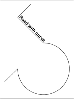
SELECT AddGeometryColumn ('public','my_geometries','my_compound_curves',
  -1,'COMPOUNDCURVE',2);
INSERT INTO my_geometries(name,my_compound_curves)
VALUES ('Road with curve',
  ST_GeomFromText('COMPOUNDCURVE((2 2, 2.5 2.5),
  CIRCULARSTRING(2.5 2.5,4.5 2.5, 3.5 3.5), (3.5 3.5, 2.5 4.5, 3 5))'));

Curvepolygon

A curvepolygon is a polygon that has an exterior or inner ring with circularstrings. In pre-1.4 PostGIS versions, compondcurves can’t be used to form rings, even though SQL-MM specs allow for such curvepolygons. The following listing and figure 2.15 show some examples of curvepolygons.

Figure 2.15. Curvepolygons generated from the code in listing 2.5

Listing 2.5. Creating curved polygons

SELECT AddGeometryColumn ('public','my_geometries',
  'my_curve_polygons',-1,'CURVEPOLYGON',2);


INSERT INTO my_geometries(name,my_curve_polygons)
VALUES ('Solid Circle', ST_GeomFromText('CURVEPOLYGON(
  CIRCULARSTRING(0 0,2 0, 2 2, 0 2, 0 0))')),
  ('Circle t hole',
  ST_GeomFromText('CURVEPOLYGON(CIRCULARSTRING(2.5 2.5,4.5 2.5,
  4.5 3.5, 2.5 4.5, 2.5 2.5),
  (3.5 3.5, 3.25 2.25, 4.25 3.25, 3.5 3.5) )') ),
('T arcish hole',
  ST_GeomFromText('CURVEPOLYGON((-0.5 7, -1 5, 3.5 5.25, -0.5 7),
CIRCULARSTRING(0.25 5.5, -0.25 6.5, -0.5 5.75, 0 5.75, 0.25 5.5))'));

PostGIS 1.4 introduced support for compoundcurves as rings in a curvepolygon. Following is the WKT of a curvepolygon with a compoundcurve outer ring and a circular-string inner ring:

CURVEPOLYGON(COMPOUNDCURVE(CIRCULARSTRING(0 0,2 0, 2 1, 2 3, 4 3),
 (4 3, 4 5, 1 4, 0 0)),
 CIRCULARSTRING(1.7 1, 1.7 0.9, 1.6 0.5, 1.4 0.6, 1.7 1))

The output of the curve polygon is shown in figure 2.16.

Figure 2.16. Compoundcurve in a curvepolygon with a circularstring hole

2.2.7. 3D geometries

PostGIS recognizes and stores 3D geometries, but full support is still spotty. As we’ve shown, you can easily create 3D points, linestrings, polygons, and curved geometries, but you must keep in mind that these lack the volumetric sense of 3D. They’re 2D objects sitting in 3D space (as such, they’re sometimes referred to as 2.5D). Be mindful of the following caveats when working with 3D geometries:

• PostGIS and the underlying GEOS library have minimal support for 3D geometries. For example, all the relationship operators check only whether two geometries relate in 2D space and completely ignore the Z dimension. Suppose you have one box floating above another and not touching; asking if the boxes intersect yields a true result because they occupy the same 2D coordinates.
• Overlay functions such as intersection and union only partially handle the third dimension. When applied to 3D geometries, they perform the expected operation on the 2D portion of the geometry and then interpolate the Z coordinate. This may be acceptable when elevations don’t need to be precise, say on a hiking trail, but in general this is unwanted behavior.
• Spatial operators achieve their amazing speed through use of bounding box indexes. Unfortunately, these indexes currently don’t extend into the third dimension. The good news is that work is being done to rectify the situation.

2.3. Summary

We began this chapter by introducing the geometry_columns metatable. Every PostGIS-enabled database has this metatable to catalog information about geometry columns in the database. We then introduced five functions that are commonly used to interact with the geometry_columns metatable, with AddGeometryColumn being the most prominent of these functions. We advised strongly against editing the geometry_columns table directly.

We then moved on to the single geometries of points, linestrings, and polygons, giving examples of their WKT representation and the INSERT SQL statements to add them to geometry_columns. Combining single geometries creates collection geometries. We covered multipoints, multilinestrings, multipolygons, and geometrycollections.

We finished the chapter with discussions of curved and 3D geometries. Because these two families of geometries are much more complex and less supported in real-world GIS modeling, they don’t fully enjoy the support of third-party tools and are only partially supported by PostGIS itself.

We hope that this chapter will give you the necessary know-how to set up your PostGIS table and to use metatables in PostGIS to centralize data type management. You should have a good understanding of single geometries and the purpose of geometry collections. In the next chapter, we’ll apply what you learned in this chapter by exploring the various approaches to organize your data in a PostGIS database.

Finally, we want to remind you not to think too much about rigorous definitions when modeling. If it looks, feels, and smells like a polygon, treat it like a polygon; don’t worry about inner rings and outer rings unless you need to. Although PostGIS tries to follow standards and the standards try to follow solid mathematical foundations, you’ll invariably run into definitional inconsistencies. Don’t be put off by these; instead, focus on what you’re trying to accomplish using PostGIS.