Chapter 10. Enhancing SQL with add-ons

 

 

In this chapter, we’ll cover common open source add-on tools that are often used to enhance the functionality of PostgreSQL. What makes these tools special is that they unleash the power of SQL, so you can write much more powerful queries than you can with PostGIS and PostgreSQL alone. They also allow for greater abstraction of logic, because you can reuse these same functions and database triggers across all your application queries.

The tools we’ll be covering are as follows:

• Topologically Integrated Geographic Encoding and Referencing (TIGER) geocoder— A geocoding toolkit with scripts for loading U.S. Census TIGER street data and approximating address locations with this data. It also contains geocoding functions on top of PostGIS functions for address matching. The benefits of using this toolkit instead of a geocoding web service are that it can be customized any way you like and you won’t incur service charges per batch of addresses geocoded.
• pgRouting— A library and set of scripts used in conjunction with PostGIS functions. pgRouting includes various algorithms to perform tasks like shortest path along a road network, driving directions, and geographic constrained resource allocation problems (aka traveling salesman).
• PL/R— A procedural language handler for PostgreSQL that allows you to write stored database functions using the R statistical language and graphical environment. With this you can generate elegant graphs and leverage a breadth of statistical functions to build aggregate and other functions within your PostgreSQL database. This allows you to inject the power of R in your queries.
• PL/Python— A procedural language handler for PostgreSQL that allows you to write PostgreSQL stored functions in Python. This allows you to leverage the breadth of Python functions for network connectivity, data import, geocoding, and other GIS tasks. You can similarly write aggregate functions in Python.

We expect that after you’ve finished this chapter, you’ll have a better appreciation of the benefit of integrating this kind of logic right in the database instead of pulling your data out to be processed externally.

10.1. Georeferencing with the TIGER geocoder

The TIGER geocoder is a suite of SQL functions that utilize TIGER U.S. Census data. The TIGER geocoder not only makes it easy to batch geocode data with SQL update statements but also provides geocoding functionality to applications via simple SQL select statements. Although the TIGER geocoder is specific to the TIGER U.S. data structure, its concepts are useful when creating your own custom geocoder for specialized data sets.

 

 

The TIGER geocoder packaged with PostGIS 1.5 and below doesn’t handle the new U.S. Census data ESRI shapefile format. For those, therefore, we’re using a newer version currently under development by Stephen Frost, which handles the new ESRI shapefile format. You can download this version from the PostGIS in Action book site, http://www.postgis.us/downloads/tiger_geocoder_2009.zip. More details on getting Steve’s latest code can be found in appendix A.

Another geocoder built for OpenStreetMap utilizes PostgreSQL functions and a C library. This one may be of more interest to people outside the United States or OSM data users, but we didn’t have time to investigate and cover it. This one is called Nominatim and can be accessed from http://wiki.openstreetmap.org/wiki/Nominatim.

For our exercises we’ve taken Steve Frost’s newer version and made some minor corrections to support the TIGER Census 2009 data. We’ve also changed the lookup table script to create skeleton tables we inherit from. We’ve introduced an additional script file called tiger_loader.sql that generates a loader batch script for Windows or Linux. We’ll briefly describe how to use this custom loader and how to test drive the geocoder functions in this section.

10.1.1. Installing the TIGER geocoder

In order to use the TIGER geocoder functionality, you need to do the following:

• Install the TIGER geocoder .sql files.
• Have Wget and UnZip (for Linux) or 7-Zip for Windows handy. These we described in chapter 7 on loading data.
• Use our loader_generate_script() SQL function that generates a Windows shell or Linux bash script. You can then call this generated script from the command line to download the specified states data, unzip it, and load it into your PostGIS-enabled database.

The details of all of this can be found in the Readme.txt file packaged with the TIGER geocoder code on the PostGIS in Action book site. Now that we’ve outlined the basic steps, we’ll go into specifics about using this loader_generate_script function to load in TIGER data.

10.1.2. Loading TIGER data

In this exercise we test out our TIGER loader. It uses a set of configuration tables to denote differences in OS platforms, tables that need to be downloaded, how they need to be installed, and pre- and post-process steps. The script to populate these configuration tables and the generation function loader_generate_script are in the file tiger_loader.sql. The key tables are as follows:

• loader_platform— This table lists OS-specific settings and locations of binaries. We prepopulated it with generic Linux and Windows records. You’ll probably want to edit this table to make sure the path settings for your OS are right.
• loader_variables— These are variables not specific to the OS, such as where to download the TIGER files, which folder to put them in, which temp directory to extract them to, and the year of the data.
• loader_lookuptables— This table of instructions shows how to process each kind of table and what tables to load in the database. You can set the load bit to false if you don’t want to load a table. For the most part, you shouldn’t need to change this.
• loader_generate_script— This function will generate the command-line shell script to download, extract, and load the data. For our example, we downloaded just Washington, D.C., data because it’s the smallest and only has one county. We did that by running the statement
  SELECT loader_generate_script(ARRAY['DC'], 'windows'), If you need more than one state and for a different OS, you would list the states as follows:
  SELECT loader_generate_script(ARRAY['DC','RI'], 'linux'), The script will generate a separate script record for each state. You can then copy and paste the result into a .bat file (remove the start and end quotes if copying from pgAdmin) and then run the shell script.

The generated scripts use Wget, 7-Zip (or UnZip), and the PostGIS-packaged shp2pgsql loader to download the files from the U.S. Census, unzip them, and load the data into a PostGIS-enabled database. For Windows users we highly suggest using 7-Zip and installing Wget for Windows, as we described in chapter 7.

For Linux/Unix/Mac OS X users, Wget and UnZip are generally in the path, so you probably don’t need to do anything aside from CD-ing into the folder where you saved your generated script. We use the states_lookup table in the tiger schema to fine-tune which specific states to download data for and generate the download path based on the new TIGER path convention. Then we have a single SQL statement that combines all these to generate either a Windows command-line or Linux bash script for the selected states.

The state/county–specific data is defaulted in the loader_variables table to store in a schema called TIGER_data. All of these will inherit from shell tables defined in the tiger schema. One set of tables for each state will be generated. Each state’s set of tables is prefixed with the state abbreviation.

We use inheritance because it’s more efficient for large data sets because it allows for piecemeal loading or reloading of data. It has the side benefit that the TIGER geo-coder doesn’t need to know about these tables to use them transparently via the skeleton parent tables we’ve set up. It also gives us the option to easily break these tables into other schemas later any way we care to.

For all this to work seamlessly, we need to make sure that the tiger schema is in our database search path.

We won’t be showing the code here because it’s too long to include, but you can download the code from the PostGIS in Action book site at http://www.postgis.us. Click the Chapter Code Download link, choose the chapter 10/TIGER_geocoder_2009 folder, and read the ReadMe.txt file for more details on how to install and get going with it.

10.1.3. Geocoding and address normalization

In this section, we’ll go over the key functions of the TIGER geocoder package.

Geocoder

The main function in the geocoder is called geocode, and it calls on many helper functions. This function is specific to the way TIGER data is organized. If you have non-U.S. data or have more granular data such as city land parcel data, you’ll need to write your own geocode function or tweak this one a bit. An example of its use is shown in the following listing.

Listing 10.1. Example of the geocode function

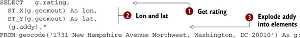
The geocode function takes an address and returns a set of records that are possible matches for the address. One of the fields in the geocode function is a rating field. For perfect matches, the rating will be 0. The greater the number, the less accurate the match. One of the objects is a complex type called norm_addy. A norm_addy object is output as a field called addy in the returned records. The norm_addy represents a perfectly normalized address where abbreviations are standardized based on the various *lookup tables in the tiger schema. In we’re exploding addy into its constituent properties so they appear as individual columns. The addy object has a property for each component of the address and is a normalized version of the closest match address. The result also includes a field called geomout, which is a PostGIS lon lat point geometry interpolated along the street segments. We display the lon lat components of this point.

If we wanted just individual elements of the addy object and not all of them, then we would write a query something like this:

Listing 10.2. Listing specific elements of addy in geocode results

In this example we also test the power of the soundex/Levenshtein fuzzy string–matching functionality by feeding invalid and misspelled addresses. In this example we get multiple results back because we fed in an example that has the wrong Zip Code and a misspelled street. In this case, we get three possible results, all with slightly different ratings. We also want to trim down the number of digits of the lon lat, so we round the digits. We first cast them to numeric because the round function expects a numeric number and PostGIS returns double precision. This casting may or may not be needed depending on which autocasts you have in place. Instead of round, we could have also used the PostGIS ST_X(ST_SnapToGrid(g.geomout, 0.00001)) to truncate the coordinates. We select specific elements out of addy and glue them together for a more appropriate output.

The result of this query is a table like table 10.1.

Table 10.1. Results of geocoding address in listing 10.2

rating	lon	lat	snum	street	zip
10	-77.04961	38.90309	1021	New Hampshire Ave	20037
12	-77.04960	38.90310		New Hampshire Ave	20036
19	-77.02634	38.93359		New Hampshire Ave	20010

Recall that you shouldn’t use lon lat data with PostGIS linear referencing and other Cartesian functions. In this case it’s more or less safe to do so because the street segments are generally so short that the approximation of the sphere projected to a flat surface (Plate Carrée projection) doesn’t distort the results too much. The longer the street segments, the more erroneous your interpolations will be. It’s also rare that street numbers are equally spaced along a street, so the interpolation is still a best guess under the assumption of a perfect distribution.

From the table, we can quickly deduce that the first record with a rating of 10 is most likely the best match. Now when geocoding a table in a batch, we may want just the first and best match plus the rating. The following listing is an update statement that will do that.

Listing 10.3. Batch geocoding with the geocode function

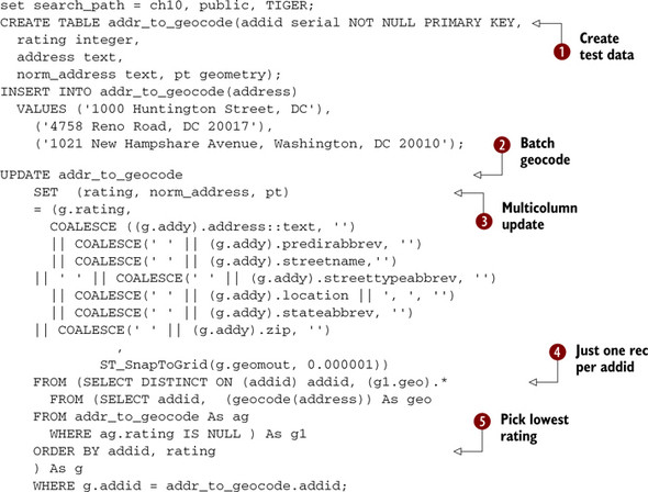
We first create some dummy addresses to geocode. Then we geocode all in the table. We’re using the ANSI SQL multi-column update syntax so we can simultaneously update the rating, norm_address, and pt with a single command. This can be broken out as well. We create a subselect using PostgreSQL’s unique DISTINCT ON feature and include only those records that we haven’t already geocoded (ag.rating is NULL). Using DISTINCT ON (addid) will guarantee that we get only one record back for each address. We order by addid and then by rating to ensure that we get the addresses with the lowest rating number.

Normalize_Address

The normalize_address function is probably the most reusable of the TIGER geocoder functions. It uses the various *lookup tables in the tiger schema to formulate a standardized address object that has each part of the address broken out into a separate field. This standardized address is then packaged as a norm_addy data type object and fed to the various geocode functions. The geocode function first does a normalize_ address of the address and then feeds it to geocode_address. Following is a demonstration of normalize_address:

SELECT foo.address As orig_addr, (foo.na).*
  FROM (SELECT address, normalize_address(address) As na
     FROM addr_to_geocode) AS foo;

Note that here again we have the strange-looking (object).* syntax to explode out the returned norm_addy object type into its individual properties.

The result of this query looks like table 10.2.

Table 10.2. Result of normalizing our test addresses

orig_addr	address	predirabbrev	streetname streettypeabrev .....
1000 Huntington Street, DC	1000	Huntington	St
4758 Reno Road, DC 20017	4758	Reno	Rd	..
:

10.1.4. Summary

In this section you learned how to load TIGER data and use the PostGIS TIGER geo-coder. We hope we’ve provided enough detail for you to put it to work.

Another common activity associated with addresses is figuring out the best route from address A to address B taking into consideration road networks. In the next section, we’ll explore using another popular tool called pgRouting. pgRouting utilizes heuristic weights you define on road networks to determine feasible and best routes to take. Weights are arbitrary costs you assign to each road element based on criteria such as whether the road requires paying a toll, whether the road is congested, its capacity for traffic, its length, and so forth.

10.2. Solving network routing problems with pgRouting

Once you have all your data in PostGIS, what better way to show it off than to find solutions to common routing problems such as the shortest path from one address to another and the traveling salesman problem (TSP). pgRouting lets you do just that. All you have to do is add a few extra columns to your existing table to store input parameters and the solution, and then execute one of the many functions packaged with pgRouting. pgRouting makes it possible to get instant answers to seemingly intractable problems. These problems are often solved with fairly expensive desktop tools such as ArcGIS Network Analyst or with web services. pgRouting allows you to solve these problems right in the database and to share them across applications.

10.2.1. Installation

In order to get started with pgRouting, you must first install the library and then run a few SQL scripts in a PostGIS-enabled database. Linux users will most likely need to compile your own. For Windows and Mac users, binaries are currently available for PostgreSQL 8.3 and 8.4. You can download the source and binaries from http://www.pgrouting.org/download.html. At the time of this writing, pgRouting 1.03 is the latest version, and you should end up with three additional library files in the lib folder of your PostgreSQL installation: librouting, librouting_dd, and librouting_tsp.

Regardless of how you obtain the files and perform the installation, you must execute a series of scripts that wrap the base functions as PostgreSQL SQL functions. Further instruction can be found in the pgRouting site and in the chapter 10 data download file. For convenience, we’ve collected them on our companion website at http://www.postgis.us.

In future versions of PostGIS after PostGIS 2.0, there are plans to integrate pgRouting into the PostGIS project similar to what has been done with the raster project. You can expect PostGIS 2.1+ versions to have routing capability as part of the PostGIS core.

10.2.2. Shortest route

The most common use of routing is to find the shortest route among a network of interconnected roads. Anyone who has ever sought driving directions from a GPS unit should be intimately familiar with this operation. For our example, we picked the North American cities of Minneapolis and St. Paul. This pair is perhaps the best known of the twin cities in the United States. We imagine ourselves as a truck driver who needs to find the shortest route through the Twin Cities. As with most cities in the world, highways usually bifurcate at the boundary of a metropolis, offering a perimeter route that encircles the city and multiple radial routes that extend into the city center to form a spokes-and-wheel pattern. The Twin Cities have one of the most convoluted patterns we could find of all the major cities in the United States. A truck driver trying to pass through the cities via the shortest route has quite a few choices to make; furthermore, the shortest choice isn’t apparent from just looking at the map; see figure 10.1. A driver entering the metropolitan area from the south and wishing to leave via the northwest has quite a few options. We’ll use pgRouting to point the driver to the shortest route.

Figure 10.1. We plot the shortest route through the Twin Cities.

To prepare your table for pgRouting, you need to add three additional columns: source, target, and length, which have already been added by the ch10_data.sql script:

ALTER TABLE twin_cities ADD COLUMN source integer;
ALTER TABLE twin_cities ADD COLUMN target integer;
ALTER TABLE twin_cities ADD COLUMN length double precision;

To populate the first two of these columns we run the assign_vertex_id function installed with pgRouting:

SELECT assign_vertex_id('twin_cities',.001,'the_geom','gid'),

This function loops through all the records, assigns the linestring two integer identifiers: one for the starting point and one for the ending point. The function makes sure that identical points receive the same identifier even if shared by multiple linestrings. In routing lingo, this process builds the network.

We next need to assign a cost to each linestring. Because we’re looking at distance, we’ll take the length of each linestring and fill in the length column:

UPDATE twin_cities SET length = ST_Length(the_geom);

Although we’re not doing it in our example, we can expand the applicability of the shortest route by using different cost factors to weigh the linestrings. For example, we could weigh highways by a speed limit so that slower highways have a higher cost. We could even get live feeds of traffic conditions so that routes with major traffic congestion would receive a high cost and provide real-time guidance to a driver.

With our network prepared and our cost assigned, all it takes is the execution of a pgRouting function to return the answer:

set search_path = public, ch10;
SELECT the_geom INTO ch10.dijkstra_result FROM dijkstra_sp('twin_cities',134,82);

Node 134 is on Interstate 35 south of the city, and node 82 is Interstate 94 northwest of the city.

The Dijkstra algorithm is one approach to arrive at an exact solution. For small networks like ours, exact solutions are possible in real time. For large networks, approximate solutions are often acceptable in the interest of computation time. pgRouting offers an A-Star algorithm to get faster but less-accurate answers. To see the ever-growing list of algorithms available (or to contribute your own), visit the main pgRouting site at http://pgrouting.postlbs.org. For large networks, we also advise that you add spatial indexes to your table prior to executing any algorithms.

The shortest-route problem is a general class of problems where you try to minimize the cost of achieving an objective by selecting the cheapest solution to the problem. The concept of cost is something that’s user defined. Don’t limit yourself to solving problems involving time and distance. For example, you can easily download a table of calories from your local McDonald’s, group the food items into sandwiches, drinks, and sides, and ask the question of the least fattening meal you can consume provided that you must order something from each group—the McRouting problem.

10.2.3. Traveling salesperson problem

Many times in our programming ventures, we’ve come across the need to find solutions to TSP-related problems. Many times we’ve given up because nothing was readily available to quickly accomplish that task. Although algorithms in many languages are available, setting up a network and pairing the algorithm with whichever database we were using at the time was much too tedious. We often resorted to suboptimal SQL-based solutions. How often have we hoped that something like pgRouting would come along!

The classic description of a TSP problem involves a salesman having to visit a wide array of cities selling widgets. Given that the salesman has to visit each city only once, how should he plan his itinerary to minimize total distance traveled?

To demonstrate TSP using pgRouting, we’ll pretend that we’re a team of inspectors from the International Atomic Energy Agency (IAEA, the United Nations’ nuclear energy watchdog) with the tasks of inspecting all nuclear plants in Spain. A quick search on Wikipedia shows that seven plants are currently operational on the entire Iberian Peninsula. We populate a new table as follows:

CREATE TABLE spain_nuclear_plants
(id serial, plant_name character varying,
lat double precision, lon double precision);

This table is included as part of the ch10–data.sql script.

For TSP, we need our table to have point geometries. Each row would represent a node that the nuclear inspector must visit. Another requirement of the TSP function is that each node must be identified using an integer identifier. For this reason, we include an id column and assign each plant a number from 1 to 7. With all the pieces in place, we execute the TSP function:

SELECT vertex_id
FROM tsp('SELECT id as source_id, lon AS x, lat AS y FROM
     spain_nuclear_plants','1,2,3,4,5,6,7',3);

This TSP function is a little unusual in that the first parameter is an SQL string. This string must return a set of records with the columns source_id, x, and y. The second parameter lists the nodes to be visited, and the final parameter is the starting node. The TSP function returns the nodes in order of the sequence of travel. The results are shown in figure 10.2.

Figure 10.2. Optimized shortest-distance travel path for visiting all nuclear power plants in Spain starting from Almaraz

Like all algorithms in pgRouting, TSP works only on a Cartesian plane. SRID doesn’t even come into play for TSP because TSP doesn’t require a geometry column. In the interest of computational speed, routing problems rarely demand exact answers. Think of the number of times your GPS guidance unit took you down an awkward path. Because of this tolerance for errors, the inexactitudes generated by not accounting for earth curvature can usually be ignored, even for large areas. Don’t apply the algorithms where your distances cover more than a hemisphere; otherwise, you’d be finding yourself trying to sail to China by crossing the Atlantic and rediscovering the New World but without any fanfare.

10.2.4. Summary

What we wanted to show in this section is the convenience brought forth by the marriage of a problem-solving algorithm with a database. Imagine that you had to solve the shortest route or TSP problem on some set of data using just a conventional programming language. Without PostGIS or pgRouting, you’d have to define your own data structure, code the algorithm, and find a nice way to present the solution. Should the nature of your data change, you’d have to repeat the process. In the next sections, we’ll explore PL languages. PL languages and SQL are another kind of marriage that combines the expressiveness of an all-purpose or domain-specific language well suited for expressing certain classes of problems with the power of SQL to create a system that’s greater than the sum of its parts.

10.3. Extending PostgreSQL power with PLs

One thing that makes PostgreSQL unique among the various relational databases is its pluggable procedural language architecture. Several people have created procedural handlers for PostgreSQL that allow writing stored functions in a language more suited for a particular task. This allows you to write database stored functions in languages like Perl, Python, Java, TCL, R, and Sh (shell script) in addition to the built-in C, PL/ PgSQL, and SQL. Stored functions are directly callable from SQL statements. This means you can do certain tasks much more easily than you would if you had to extract the data, import them into these language environments, and push them back into the database. You can write aggregate functions and triggers and use functions developed for these languages right in your database. These languages are prefixed with PL: PL/Perl, PL/Python, PL/Proxy, PL/R, PL/Sh, PL/Java, and so on. The code you write is pretty much the same as what you’d write in the language except for the additional hooks into the PostgreSQL database.

10.3.1. Basic installation of PLs

In order to use these non-built-in PL languages in your database, you need three basic things:

• The language environment installed on your PostgreSQL server
• The PL handler .dll/.so installed in your PostgreSQL instance
• The language handler installed in the databases you’ll use them in—usually by running a CREATE LANGUAGE statement

The functionality of a PL extension is usually packaged as a .so/.dll file starting with pl*. It negotiates the interaction between PostgreSQL and the language environment by converting PostgreSQL datasets and data types into the most appropriate data structure for that language environment. It also handles the conversion back to a PostgreSQL data type when the function returns with a record set or scalar value.

10.3.2. What can you do with a non-native PL

Each of the PL languages has various degrees of integration with the PostgreSQL environment. PL/Perl is perhaps the oldest and probably the most common and most tested you’ll find. PLs are registered in two flavors: trusted and untrusted. PL/Perl can be registered as both trusted and untrusted. Most of the other PLs offer just the untrusted variant.

 

 

In the sections that follow, we’ll demonstrate PL/Python and PL/R. We’ve chosen these particular languages because they have the largest offerings of spatial packages. We also think they’re pretty cool languages. They’re favorites among geostatisticians and GIS programmers. Both languages have only an untrusted flavor.

Python is a dynamically typed, all-purpose procedural language. It has elegant approaches for creating and navigating objects, and it supports functional programming, object-oriented programming, building of classes, meta programming, reflection, map reduce, and all those modern programming paradigms you’ve probably heard of. R, on the other hand, is more of a domain language. R is specifically designed for statistics, graphing, and data mining. It has a fairly large cult following among research institutions. It has many built-in statistical functions or functions you can download and install via the built-in package manager. Most of the functionality it offers you’ll not find anywhere else except possibly in pricey tools such as SAS and MATLAB. You’ll find tasks such as applying functions to all items in a list, doing matrix algebra, and dealing with sparse matrices—fairly short and sweet to do in R once you get into the R mindset. In addition to manipulating data, R has a fairly extensive graphical engine that allows you to generate elegant-looking graphs with only a few lines of code. You can even do 3D plots.

You can write functions in PL/Python and PL/R that pull data from the PostgreSQL environment and have them return simple scalars or more complex sets. You can even return binary objects such as image files. In addition, you can write database triggers in PL/Python and PL/R that use the power of these environments to run tasks in response to changes of data in the database. For example, you can geocode data when an address changes or have a database trigger to regenerate a map tile on a change of data in the database without ever touching the application edit code. This feature is next to impossible to do with just the languages and a database connection driver. In addition, you can write aggregate functions with these languages that will allow you to feed the sets of rows to aggregate and use functions available only in these languages to summarize the data. Imagine an aggregation function that returns a graph for each grouping of data. You can find some examples of this listed in appendix A.

In the sections that follow, we’ll write some stored functions in these languages. These examples will have only a slight GIS bent. Our intent here is to show you how to get started integrating these in your PostgreSQL database and give you a general feel of what’s possible with these languages. Only your imagination limits the possibilities you can achieve with this kind of intimate integration. We’ll also show you how you can find and install more libraries that you can utilize from within a stored function.

10.4. Graphing and accessing spatial analysis libraries with PL/R

PL/R is a stored procedural language supported by PostgreSQL that allows you to write PostgreSQL stored functions using the R statistical language and graphical environment. You can call out to the R environment to do neat things like generate graphs or leverage a large body of statistical packages that R provides. R is a favorite among statisticians and researchers because it makes flipping matrices, aggregation, and applying functions across rows and columns and other data structures almost trivial. It also has a breath of options for data import from various formats and has many contributed packages available for geospatial analysts. We’ll just touch the surface of what PL/ R and R provide. In order to get deeper into the R trenches, we suggest reading the Manning book R in Action by Robert I. Kabacoff or Applied Spatial Data Analysis with R by Roger S. Bivand, Edzer J. Pebesma, and V. Gómez-Rubio. Check out appendix A for other useful R sites and examples.

For the exercises that follow, we’ll use R 2.10. Most of these should work on lower versions of R as well.

10.4.1. Getting started with PL/R

In order to write PostgreSQL procedural functions in R, you must do the following:

• Install the R environment on the box your PostgreSQL service/daemon runs on. R is available for Unix, Linux, Mac OS X, as well as Windows. Unix/Linux users may need to compile plr. For Windows and Mac OS X users, there are precompiled binaries. Any R from version R 2.5 through R 2.11 should work fine. We’ve tested it against R 2.5, R 2.6, and R 2.11. You can download source and precompiled binaries of R from http://www.r-project.org/. After the install, check your environment variables to make sure R_HOME is specified correctly. This is what PL/R uses to determine where R is installed and should be called from.
• Compile/install the plr.so/.dll files by copying this file into the lib directory of your PostgreSQL install. If you’re using an installer, this is probably already done for you. If you’re running under Linux, R should be configured with the option -enable-R-shlib. Note that you must use the version compiled for your version of PostgreSQL. You can download the binaries and source from http://www.joeconway.com/plr/. You may need to restart the PostgreSQL service before you can use PL/R in a database.
• Run the packaged plr.sql file in the PostgreSQL database in which you’ll be writing R stored functions. You need to repeat this step for each database you want to R enable.

If any of this is confusing or you get stuck, check out PL/R wiki installation tips guides at http://www.joeconway.com/web/guest/pl/r/-/wiki/Main/Installation+Tips.

 

 

10.4.2. Saving datasets and plotting

Now we’ll take PL/R for a test drive. For these exercises, we’ll use R 2.10.1, but any of these should work in lower versions of R.

Saving PostgreSQL Data to RData Format

For our first example, we’ll pull data out of PostgreSQL and save it to R’s custom binary format (RData). There are two common reasons to do this:

• It makes it easy to interactively test different plotting styles and other R functions in R’s interactive environment against real data before you package them in a PL/R function.
• If you’re teaching a course and are using R as a tool for analysis, you may want to provide your datasets in a format that can be easily loaded in R by students. For that reason, you may want to create PL/R functions that dump out data in self-contained problem set nuggets.

For this example we’ll use the PostgreSQL pg.spi.exec function and R’s save function. The pg.spi.exec function is a PL function that allows you to convert any PostgreSQL dataset into a form that can be consumed by the language environment. In the case of PL/R this is usually an R data.frame.

The save command in R allows you to save many objects to a single binary file, as shown in listing 10.4. These objects can be dataframes (including spatial dataframes), lists, matrices, vectors, scalars, and all of the various object types supported by R. When you want to load these in an R session, then you run the command load(“filepath”).

Listing 10.4. Saving PostgreSQL data in R data format with PL/R

In this example, we create two datasets that contain Washington, D.C., counties and Zip Codes. We then save this to a file called dc.RData. RData is the standard suffix for the binary R data format, and in most desktop installs when you launch it, it will open R with the data loaded.

To run this save example, we run SELECT ch10.save_dc_rdata();.

We can load this data in R by clicking the file or by opening R and running a load call in R. Following are a couple of quick commands to try in the R environment:

To load a file in R:

load("C:/temp/dc.RData")

To list contents of file in R:

ls()

To view a data structure in R:

summary(dczips)

To view data in R, type the name of the data variable:

dccounties

To view a set of rows in a variable in R:

dczips[1:3,]

To view columns of data in R variable:

dczips$zcta5ce

These R commands demonstrate some commonly used constructs in R. Though not demonstrated, if you use the variable <- syntax, data gets assigned to an R variable instead of printed to the screen. Figure 10.3 is a snapshot of the commands we described.

Figure 10.3. Demonstration output of running the previous statements in R

One task that R excels in is drawing plots. Many people, even those who don’t care about statistics, are attracted to R because of its sophisticated scriptable plotting and graphing environment. In the next listing, we demonstrate a bit of this by generating a random data set in PostgreSQL and plotting it using PL/R.

Listing 10.5. Plotting PostgreSQL data with R

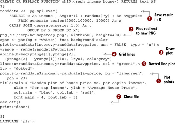
In this code we’re creating a stored function written in PL/R that will create a file called housepercap.png on the C:/temp folder of our PostgreSQL server. We first create random data by running an SQL statement using the PostgreSQL generate_series function and dump this in the randdata R variable. We then create a PNG file (note other functions such as pdf, jpeg, and the like can be used to create other formats), which all the plotting will be redirected to. We then draw our plot. The n type means no plot; it just prepares the plot space so that we can then draw grid lines , lines, and points on the same grid. We close writing to the file with dev.off() and then return text saying “done.”

 

 

You run the previous function with an SQL statement:

SELECT ch10.graph_income_house();

When it’s done, it will return “done.” Running this command generates a PNG file, as shown in figure 10.4.

Figure 10.4. Result of SELECTch10.graph_income_house()

10.4.3. Using R packages in PL/R

The R environment has a rich gamut of functions, data, and data types you can download and install. All the functions and data structures are distributed in packages that are often referred to as libraries. When a package is installed, it becomes a library folder you can see in the library folder of your R installation. R makes finding, downloading, and installing additional libraries easy using the Comprehensive R Archive Network (CRAN). Once a package is installed in R, you can then use it in PL/R functions.

What’s particularly nice about the R system is that many packages come with demos that show the features of the package. Commands to view these demos are shown in table 10.3. They also often come with something called vignettes. Vignettes are quick tutorials on using a package. Demos and vignettes make R a fun, interactive learning environment. In order to use a vignette or demo, you first have to use the library command to load the library.

Table 10.3. Commands for installing and navigating packages

Command	Description
library()	Gives a list of packages already installed
library(packagename)	Loads a package into memory
update.packages()	Upgrades all packages to latest version
install.packages(“packagename”)	Installs a new package
available.packages()	Lists packages available in default CRAN
chooseCRANmirror()	Allows you to switch to a different CRAN
demo()	Shows list of demos in loaded packages
demo(package = .packages(all.available = TRUE))	Lists all demos in installed packages
demo(nameofdemo)	Launches a demo (note that you must load lib first)
help(package=somepackagename)	Gives summary help about a package
help(package=packagename, functionname)	Gives detailed help about an item in a package
vignette()	Lists tutorials in packages
vignette(“nameofvignette”)	Launches a PDF of exercises

In order to test the CRAN install process, we’ll install a package called rgdal, which is an implementation of the Geospatial Data Abstraction Library (GDAL) for R. You saw GDAL in chapter 7 on data loading. rgdal relies on another package called sp. The R install process automatically downloads and installs dependent packages as well, so there’s no need to install sp if you install rgdal. In addition to supporting vector data using OGR commands, GDAL also supports raster data.

To install packages in R, we use the R command line or Rgui:

• At a command line type R (or Rgui).
• Once in the R environment, type the following:

To launch R:

R

To load the rgdal library:

library(rgdal)

If prior command failed, use the next commands to install rgdal and then load it:

install.packages("rgdal")
library(rgdal)

To get help about the rgdal library:

help(package=rgdal)

To quit out of the R console:

q()

 

 

Next we’ll test drive our rgdal installation with a couple of exercises.

10.4.4. Quick primer on rgdal

In order to test our rgdal installation, we’ll run the following commands in R and then wrap some of this functionality in a PL/R function.

To load the rgdal library:

library(rgdal)

To get a list of raster drivers:

gdalDrivers()

To get list of vector geometry drivers:

ogrDrivers()

To return structure details about the gdalDrivers list:

str(gdalDrivers())

str() is an R base function that provides structure details about an R object. In the case of data.frames, which are similar in concept to relational tables, it outputs the fieldnames and lengths in addition to a few other summary details.

Now we’ll make the gdalDrivers list queryable from within PostgreSQL by creating a short PL/R function, as shown in the next listing.

Listing 10.6. Function to get list of supported rgdal raster formats

We created a function called r_getgdaldrivers(), which returns just the long name field of the data.frame returned by the gdalDrivers function. Because the return type is a set of text, we can use the function as we would any other one-column table. In we do just that. The output of is shown in table 10.4.

Table 10.4. Result of r_getgdaldrivers() function

Driver
ARC Digitized Raster Graphics
Arc/Info ASCII Grid
Arc/Info Binary Grid
EUMETSAT Archive native (.nat)

In this example we output a whole column of the data.frame. For large data.frames or other kinds of R data objects, you’ll probably output just a subset of rows. For the next example, shown in listing 10.7, we’ll create a function that allows us to query if a format is updateable or copyable. In this next example we’ll demonstrate the use of the built-in R function subset, which behaves much like a SELECT SQL statement. We’ll also demonstrate passing arguments to PL/R functions.

Listing 10.7. Demonstrating subset and c functions in R

This example demonstrates both the subset() and c() functions in R. We create an overloaded function that will allow us to select just those drivers that are fitting for our create and copy functions. The subset() function is similar in concept to an SQL WHERE clause. The first argument is the data set we select from (parallel to a table in SQL), the next defines the WHERE condition with & instead of AND, and the select designates the columns of data to select. The c() function in R returns a vector. In this case we want a vector composed of just one column (the long_name). Also note that the arguments for the function are used by name without any typecasting. PL/R automatically converts from a PostgreSQL boolean to an R boolean. In the second code snippet, we test our new overloaded function r_getgdaldrivers to list only those drivers that support both copy and create.

In the next example, we’ll start to use the drivers. We’ll create a PL/R function that will read the metadata of a raster file and return a summary. One of the nice things about GDAL is that in most cases it can determine which driver to use by the file extension.

Listing 10.8. Reading metadata from image files with rgdal

In this example we create a PL/R function that will return a set of key-value pairs that represent our metadata. We first create a data type to hold our results. Ideally we would have used OUT parameters for this, but PL/R and OUT parameters don’t work well together when dealing with sets. To use rgdal we first load the library. The GDAL_info call reads all the metadata from our image and loads it into a GDAL object, which is an atomic vector. We then run the labels to grab all the labels from the vector file and use this to index and pick up the elements. To return the data as a set of properties that can be read like a table, we coerce our data into a data.frame, filling the key column with the labels and the value column with the elements. Note that the naming of the columns of our data.frame mirrors the gdalinfo_values data type. To run the function we do the following:

SELECT *  FROM r_getimageinfo('C:/Winter.jpg') As v;

The result is shown in table 10.5.

Table 10.5. Result of r_getimageinfo function call

Key	Value
rows	600
columns	800
bands	3
:

10.4.5. Getting PostGIS geometries into R spatial objects

The sp package contains various classes that represent geometries as R objects. It has lines, polygons, and points. It also has spatial polygon, line, and point data frames. Spatial data frames are similar in concept to PostgreSQL tables with geometry columns. Pushing PostGIS data into these spatial data frames and spatial objects is unfortunately not easy at the moment.

There are two approaches you can use to push geometry data into these Spatial-Polygons, SpatialLines, and other such constructs:

• Use a version of rgdal compiled with support for the PostGIS OGR driver and then use the readOGR method of rgdal, as documented here: http://wiki.intamap.org/index.php/PostGIS. There are two obvious problems with this approach. Most precompiled versions of rgdal aren’t compiled with the PostGIS driver. The other problem is that it requires you to pass in the connection string to the database. Having to specify the connection to the database that a PL/R function is running in somewhat defeats the purpose of using PL/R. If you were using it to build an aggregate function, the whole thing would be next to impossible to manage.
• The second approach is to reconstitute an R spatial object from the points of a PostGIS geometry. There are a couple of ways of doing this, such as parsing WKT/WKB or just exploding the geometries into points. We’ve chosen the explode approach using the function ST_DumpPoints introduced in PostGIS 1.5 and will demonstrate this. These exercises will work only in PostGIS 1.5+, but if you need to use a lower version of PostGIS, you can implement your own ST_DumpPoints or copy one available in PostGIS 1.5. Note that the PostGIS 1.5 version of ST_DumpPoints is implemented as a PL/PgSQL function, so it’s fairly simple to copy to a PostGIS 1.4 database.

For our first example, we’ll convert our Twin Cities pgRouting results into R spatial objects so that we can plot them in R.

Listing 10.9. Plotting linestrings with R

For this example we run a PostgreSQL query that explodes the street segments into points. We run another query , which gives us the points for the results of Dijkstra pgRouting procedure. Comments in R are denoted by #, similar to Python. We regroup points into sp lines and then lines into SpatialLinesDataFrames.

We then load the R data.frame coming out of SpatialLinesDataFrames to plot on the same axis. Figure 10.5 shows the result of running the following query:

Figure 10.5. pgRouting Twin Cities results plotted with PL/R

SELECT ch10.plot_routing_results();

 

 

The sp package has its own plot function as well, called spplot. spplot does additional things the regular R plot doesn’t. spplot is specifically targeted for spatial data, and we encourage you to explore it. You will see some fancy plots you can create with spatial data by running the following commands from R GUI console:

library(sp)
demo(gallery)

10.4.6. Outputting plots as binaries

In all plotting examples we’ve used, we’ve saved the plots to a folder on the server. This approach is fine if you’re using PL/R to generate canned reports for later distribution. If, however, you need to output to a client such as a web browser, you need to be able to output the file directly from the query. We’re aware of three approaches:

• The first uses RGtk2 and a Cairo device. This approach is documented on the PL/R wiki and requires installing both the RGtk2 and Cairo libraries. In this approach you output a graph as a bytea. The problem we’ve found with this approach is that those two libraries are fairly hefty and require installation of another graphical toolkit called GTK. The other issue is that, as of this writing, it seems to crash in PL/R during the library-load process when PL/R PostgreSQL is running, at least under Windows. The benefit of this approach, however, is that it produces nicer-looking graphics and also prevents temporary file clutter, because it doesn’t ever need to save to disk. It’s also a one-step process.
• The next approach is to save the file to disk and let PostgreSQL read the file from disk. There’s a superuser function in PostgreSQL called pg_read_file(..), but that’s limited to reading files from the PostgreSQL data cluster. One simple way to do this is to create a dummy tablespace—we’ll call it r_files—and save all R-generated files to there and then use pg_read_file to get at these files.
• Another approach is to use a PL language with more generic access to the file-system such as PL/Python or PL/Perl. Doing so requires that you wrap your PL/ R function in another PL function.

In the next section, we’ll show off another PL called PL/Python. Python is another language favorite of GIS analysts and programmers. These days, most popular GIS toolkits have Python bindings. You’ll see its use in open source GIS desktop and web suites such as Quantum GIS, OpenJUMP, GeoDJango, and even in commercial GIS systems such as Safe FME and ArcGIS.

10.5. PL/Python

PL/Python is the procedural language handler in PostgreSQL that allows you to call Python libraries and embed Python classes and functions right in a PostgreSQL database. A PL/Python stored function can be called in any SQL statement. You can even create aggregate functions and database triggers with Python. In this section we’ll show some of the beauties of PL/Python. For more details on using Python and PL/ Python, refer to appendix A.

10.5.1. Installing PL/Python

For the most part, you can use any feature of Python from within PL/Python. This is because the PostgreSQL PL/Python handler is a thin wrapper that only negotiates the messaging between PostgreSQL and the native Python environment. This means that any Python package you install can be accessed from your PL/Python stored functions. Unfortunately, not all database data types to PL/Python object mappings are supported. This means you can’t return some complex Python object back to PostgreSQL unless it can be easily coerced into a custom PostgreSQL data type.

 

 

In order to use PL/Python, you must have Python installed on your PostgreSQL server machine. Because PL/Python runs within the server, any client connecting to it such as a web app or a client PC need not have Python installed to be able to use PostgreSQL stored functions written in PL/Python. The precompiled PostgreSQL 8.3 PL/ Python libraries packaged with most distros of Windows/Mac/Linux are compiled against Python 2.4, 2.5, or 2.6. These work only with the Python minor version they were compiled against.

 

 

If you’re using the PostgreSQL Yum repository for the PostgreSQL installation, you can get PL/Python by doing this:

yum install postgresql-plpython

On most Linux/Unix machines, you can determine which version of Python PL/ Python is compiled against by doing this:

cd /
locate plpython.so
ldd path/to/plpython.so

 

 

Once you have Python and the PL/Python.so/.dll installed on your server, run the following statement to enable the language in your database:

CREATE PROCEDURAL LANGUAGE
'plpythonu' HANDLER plpython_call_handler;

If you run into problems enabling PL/Python, please refer to our PL/Python help guide links in appendix A. The common issue people face is that the required version of Python isn’t installed on the server or the plpython.so/.dll file is missing.

10.5.2. Our first PL/Python function

In order to test our PL/Python install, we’ll write a simple function that uses nothing but built-in Python constructs.

Listing 10.10. Compute sum of range of numbers

In this example, we define a PL/Python function that takes start and end numbers to define a range. We first define a simple function that adds two numbers, and then we use the built-in Python reduce construct and range construct to construct an array of numbers between the start and end values and then apply our add function to the resulting sequence.

To test this example, we can do the following:

SELECT python_addreduce(1,4);

This gives us an answer of 10.

10.5.3. Using Python packages

The Python standard installation comes with only the basics. Much of what makes Python useful is the large range of free packages for things like matrix manipulation, web service integration, and data import. A good place to find these extra packages is at the Python Cheeseshop package repository.

In order to use these packages, we’ll use the Python Cheeseshop package repository and the setup tool called Easy Install.

Easy Install is a tool for installing Python packages. You can download the version for your OS and version of Python from http://pypi.python.org/pypi/setuptools#downloads or use your Linux update tool to install it.

 

 

Now we’ll move on to installing some packages and creating Python functions using these packages.

Importing An Excel File With PL/Python

For this example, we’ll use the xlrd package, which you can grab from the Python Cheeseshop: http://pypi.python.org/pypi/xlrd.

This package will allow you to read Excel files in any OS. It doesn’t have any additional dependencies, uses the standard setup.py install process, and, for Windows users, has a setup.exe file as well. For this exercise, we’ll install it from the command line, which should work for most any OS if you’ve installed easy_install: easy_install xlrd.

We’ll test our installation in listing 10.11 by importing a test.xls file that has a header row and three columns of data. Unfortunately, PL/Python doesn’t support returning SETOF rows like PL/PgSQL, so we’ll need to create a type to store our data.

First we create a PostgreSQL data type to store our returned result so we can get back more than one value from the function:

CREATE TYPE ch10.place_lon_lat AS (
  place text, lon float, lat float);

Then we create a table to store our returned results:

CREATE TABLE imported_places(place_id serial PRIMARY KEY,
  place text, geom geometry);

Listing 10.11. PL/Python function to import Excel data

We import the xlrd package so we can use it. We’ll assume there’s data in only the first spreadsheet. We loop through the rows of the spreadsheet, skipping the first row and using the Python yield function to append to our result set. In the final yield, the function will return with all the data. Now we can use this data by inserting into a table and creating point geometries:

INSERT INTO imported_places(place, geom)
SELECT f.place, ST_SetSRID(ST_Point(f.lon,f.lat),4326)
FROM ch10.fngetxlspts('C:/temp/Test.xls') AS f;

We’re doing an insert using the Excel file as the FROM source. Because the server is running the Python code and running under the context of the postgres daemon account, the Excel file path has to be accessible by the postgres daemon account.

Importing Several Excel Files With SQL

Now let’s imagine you have several Excel files you got from a vendor, all with the same structure. They’re all in one folder and you want to import them all at once. Sometimes they even dare to give you duplicated rows that are distinct in each file but repeated in other files. Here’s where the real beauty of a PL married with SQL comes in.

First we’ll create a Python function that lists all the files in a directory. Then we’ll write another query to treat this list like a table to filter, and finally we’ll write one SQL function to insert all the data using this list.

We’ll create a function that lists the files in a passed-in directory path and returns rows of text:

CREATE FUNCTION ch10.list_files(param_filepath text)
  RETURNS SETOF text AS
$$
  import os
  return os.listdir(param_filepath)
$$
LANGUAGE 'plpythonu' VOLATILE;

The import os allows us to use all the operating system–specific functions.

PL/Python takes care of converting the Python list object to a PostgreSQL set of text objects.

Then we use the function in a SELECT statement, much like we can do with any table, applying LIKE to the output to further reduce the records we get back:

SELECT file
FROM ch10.list_files('/temp') As file
WHERE file LIKE '%.xls';

In our next example, we’ll use this list to pass to our Excel import function to get a distinct set of records. For this example we have to use a small hack to allow us to use the set-returning Excel export function in the SELECT part of our query. For PostgreSQL 8.4+, this hack is no longer needed for PL/PgSQL and PL/Perl, but it still seems to be needed for PL/Python. The hack is to wrap the Python function in an SQL function wrapper.

CREATE OR REPLACE FUNCTION ch10.fnsqlgetxlspts(param_filename text)
  RETURNS SETOF ch10.place_lon_lat AS
$$
  SELECT * FROM ch10.fngetxlspts($1);
$$
 LANGUAGE 'sql' VOLATILE;

The whole purpose of this hack is to allow us to use a non-SQL/C set-returning function in the SELECT clause instead of the FROM clause of an SQL statement. This allows for row expansion. We documented the technique at http://www.postgresonline.com/journal/index.php?/archives/16-Trojan-SQL-Function-Hack-A-PL-Lemma-in-Disguise.html.

Now for the real work:

INSERT INTO ch10.imported_places(place, geom)
SELECT place, ST_SetSRID(ST_Point(lon,lat),4326)
FROM (
SELECT DISTINCT (ch10.fnsqlgetxlspts('/temp/' || file)).*
  FROM ch10.list_files('/temp') AS file
  WHERE file LIKE 'Test%.xls'
  ) As d;

This example is similar to our last, except that we’re doing three interesting things. For each file in our Temp directory that starts with Test and ends with .xls, we’re importing the data into our places table, but we’re only importing distinct values across all the files, using the DISTINCT SQL predicate.

10.5.4. Geocoding with PL/Python

If perchance you have the need to geocode but don’t want to manage all that data, PL/Python is a great tool for enabling geocoding within your database using a third-party service such as Google Maps, MapQuest, Yahoo Maps, or Bing. You can find numerous Python packages at the Cheeseshop to do just that. One example is the googlemaps package, which you can download from http://pypi.python.org/pypi/googlemaps/1.0.2 and either run the Windows setup if you’re on Windows or compile it yourself on Linux. This particular package contains a geocoder, driving directions, and reverse geocoder functionality. Once you have the package installed, you can run the following exercises.

 

 

For this example, we’ll create a geocode function and geocode the same test addresses we did earlier.

First we create a PostgreSQL data type to return our results:

CREATE TYPE ch10.google_lon_lat AS (lon numeric, lat numeric);

Then we define a function using the Google Maps library that takes a text address and returns the lon lat location using the defined type:

CREATE FUNCTION ch10.google_geocode(param_address text) RETURNS
     ch10.google_lon_lat
AS
$$
 from googlemaps import GoogleMaps
 gmaps = GoogleMaps()
 arg_lat, arg_long = gmaps.address_to_latlng(param_address)
 return (arg_long, arg_lat)
$$
language 'plpythonu';

Now we can use that function in an SQL statement similar to how we used our TIGER geocoder function:

SELECT address, (foo.g).lon, (foo.g).lat
FROM (
    SELECT address,
      ch10.google_geocode(address) As g
FROM ch10.addr_to_geocode) AS foo;

The result of our query is shown in table 10.6.

Table 10.6. Results of our Google Maps geocoder

address	lon	lat
1000 Huntington Street, DC	-77.075906	38.957687
:

If we were to use this googlemaps class in Python outside of PostgreSQL, we would have to take these steps:

.  Establish a connection to our PostgreSQL database with a few lines of Python code and a connection string.

.  Pull the data out of our database.

.  Loop through the database, retrieve the value for each record, geocode it, and update the database with the computed values.

By packaging our Python code as a stored function, we can reuse this same function easily in every query we have by writing a simple SELECT or UPDATE statement. We can even use it in reporting tools that don’t have access to Python. We can also include it in a trigger to geocode an address when the address changes in the database.

10.6. Summary

In this chapter, we introduced various tools to enhance the functionality of PostGIS and PostgreSQL without ever leaving the database. We demonstrated loading TIGER data for geocoding and using the geocoder functions provided by the TIGER geo-coder scripts to geocode data with SQL. We then went on to demonstrate how you can solve routing problems with just SQL using pgRouting. We showed off a small bit of what you can accomplish with PL/R and PL/Python. We also demonstrated how to tap into the extensive network of prepackaged functions that R and Python offer and use them directly from PostgreSQL. We hope we piqued your curiosity enough that you’ll further explore these tools and discover what other treats they hold in store.

Next we’ll talk about another set of server-side tools. These tools are for displaying GIS data to the world and allowing the world to edit your data via a web interface or desktop tool. In the following chapter, we’ll leave the safe confines of our database and expose more of our data to the world to see and enjoy.