
Chapter 3. Organizing spatial data
In the last chapter we did a walkthrough of all the possible geometry types PostGIS offers and how you would create and store them. In this chapter we continue our study by demonstrating the different table layouts you can design to store spatial data. Next, we apply our various design approaches to a real-world example. We finish the chapter with a discussion and examples of using rules and triggers to manage inserts and updates in our tables and views.
3.1. Spatial storage approaches
You should now have a good understanding of all the spatial vector types available in PostGIS. We’ll move on to the various options for designing your database to store these types. As with any database design, there’s a healthy dose of compromise. Many considerations factor into the final structure you settle on for your spatial database such as the analysis it must support, the speed of the queries, and so forth. With a spatial database, a few additional considerations enter the design process: availability of data, the precision to which you need to store the data, and mapping tools that you need to be compatible with. Unlike databases with numerical and text data, where a poor design leads to slow queries, a poor design in a spatial database could lead to queries that will never finish in your lifetime. It also goes without saying that many factors can’t be determined at the outset: You may not know exactly how many or what type of geometry will eventually reside in the database. You may not even know how the users will query the data. As with all decision making, you do the best you can with the information you have at the time. You can always rework your design as needs change, but as any database practitioner knows, getting the design more or less right the first time saves hassle down the road.
In this section, we cover three common ways to organize data in a spatial database: heterogeneous geometry columns, homogeneous geometry columns, and inheritance. We’ll explain how you’d go about setting up your database structure using each of these approaches and point out the advantages and disadvantages. These approaches are by no means exhaustive, and you should feel free to find your own hybrid that fits your specific needs. We’ll also mainly focus on geometry data types over geography data types. Geometry data types are by far the predominant data types in PostGIS. For one thing, geometry data types have been around since the dawn of PostGIS, whereas geography data types are a recent addition. The number of functions and third-party tools supporting geometry types far outnumber those for geography types. Finally, geometry types are inherently faster for most spatial computations. All this may change as geography data types mature. On the other hand, you’ll find the general concepts we cover in this section applicable to geography types too.
3.1.1. Heterogeneous geometry columns
This approach doesn’t care about constraining columns to a specific kind of geometry. For example, to store geographic features in a city, you could create a points-of-interest column in PostGIS, set its data type to be geometry or geography, and be done. In this single column you can store points, linestrings, polygons, collections, or any other vector type for that matter. You may wish to do this if you’re more interested in geographically partitioning the city. For example, Washington, D.C., as well as many other planned cities, is divided into quadrants: NW, SW, SE, NE. A city planner can employ a single table with quadrant names as a text column and another generic geometry column to store the geometries within each quadrant. By leaving the data type as the generic geometry type, the column can store polygons for the many polygonal-shaped government edifices in D.C., linestrings to represent major thoroughfares, and points for metro stations.
There are varying degrees of the heterogeneous approach. Using a generic geometry column doesn’t necessarily mean having no additional constraints. You should still judiciously apply the constraints to ensure data integrity. We advise that you at least enforce the spatial reference system constraint and the coordinate dimension constraint because the vast majority of all non-unary functions in PostGIS and all aggregate functions require that the spatial reference system and the coordinate dimension of the input geometries be the same.
Pros
Following are the pros of the heterogeneous column approach:
- It allows you to run a single query of several features of interest without giving up the luxury of modeling them with the most appropriate geometry type.
- It’s simple. You could conceivably cram all your geometries into one table if their non-spatial attributes are more or less the same.
- Table creation is quick because you can do it by setting the field as a geometry with a single CREATE TABLE statement and not have to worry about the additional need to apply the AddGeometryColumn function. This is particularly handy if you’re trying to iteratively load data from a large number of tables and you don’t care or know what geometry types each contains.
Cons
And here are the cons of the heterogeneous column approach:
- You run the risk of having someone insert an inappropriate geometry for an object. For example, if you’ve obtained data of subway stations that should be modeled as points, an errant linestring in the data could enter your heterogeneous table. Furthermore, if you don’t constrain the spatial reference system or coordinate geometry and unwittingly end up with more than one of each, your queries could be completely incorrect or break.
- Many third-party tools can’t deal with heterogeneous geometry columns. As a workaround, you may need to create views against this table to make it appear as separate tables and add a geometry type index or ensure that your queries select only a single type of geometry type from the heterogeneous column.
- For cases where you need only to extract a certain kind of geometry, you’ll need to constantly filter by geometry type. For large tables, this could be slow and annoying to have to keep doing over and over again.
- Throwing all your geometry data into a single table could lead to an unwieldy number of self-joins. For example, suppose you placed points of interest in the same table as polygons outlining city neighborhoods; every time you need to identify which points of interest (POIs) fall into which neighborhood, you’ll need to perform a self-join on this table. Not only are self-joins taxing for the processor, they’re also taxing for the mind. Imagine a scenario where you have 100 POIs and two neighborhoods, for a total of 102 records. Determining which POIs fall into which city requires that a table of 102 rows be joined with a table of 102 rows (itself). If you had separated out the cities into their own table, you’d only be joining a table of 100 rows with a table of just two rows.
With the disadvantages of heterogeneous storage approach fresh in your mind, let’s move on to the homogenous geometry columns approach.
3.1.2. Homogeneous geometry columns
This approach avoids the mixing of different geometry types in a single column. Polygons must be stored in a column of only polygons, linestrings in linestring columns, and so on. This means that each geometry type must reside in its own column at the least, but it’s also common to break up different geometry types into entirely separate tables.
If in our D.C. example we care more about the type of the features than the quadrant each feature is located in, we’ll employ the homogeneous columns design. One possible table structure would be to define a features table with a name column and three geometry columns. We’d constrain one column to store only points, one to store only linestrings, and one to store only polygons. If a feature is point data, we’d populate the point column, leaving the other two columns null; if it’s linestring data, we’d populate the linestring column only, and so on. We don’t necessarily need to cram all of our columns into a single table. A more common design would be to use three distinct tables, one to exclusively store each type of geometry.
We now summarize the pros and cons of the homogeneous columns approach.
Pros
The homogeneous geometry columns approach offers the following benefits:
- It enforces consistency and prevents unintended mixing of geometry types.
- Third-party tools rely on consistency in geometry type. Some may go so far as to only allow one geometry column per table. The popular ESRI shapefile supports only one geometry per record, so you’d need to explicitly state the geometry column should you ever need to dump data into ESRI.
- In general, you get better performance when joining tables having large geometries and few records with tables having smaller geometries and many records than vice versa.
- When you need to draw different kinds of geometries at different Z levels, the speed is much better if you split your data into multiple tables, with each geometry type in a separate table.
- Should you be working with monstrous datasets, separate tables also allow you to reap the benefits from placing your data on separate physical disks for each table by means of tablespaces.
In PostgreSQL a tablespace is a physical folder location as opposed to a schema, which is a logical location. (Oracle also has tablespaces, and SQL Server has a similar concept called file groups.) In the default setup, all the tables you create will go into the same tablespace. As your tables grow, you may want to create additional tablespaces, each on a separate physical disk, and distribute your tables across different tablespaces to achieve maximum disk I/O. One common practice is to group rarely used tables into their own tablespace and place them on a slow disk. In PostgreSQL 9.0 tablespaces were enhanced to allow you to set random_page_cost and seq_page_cost settings for each tablespace. In older versions you could set these only at the server or database level. The query planner uses these two parameters to determine how to rate query paths based on whether they utilize data running on slower disks or faster disks.
Cons
On the con side, by choosing the homogeneous geometry columns approach, you may face the following obstacles:
- When you need to run a query that draws multiple geometry types, you have to resort to a union query. This can add to the complexity and the speed of the query. For example, if 99% of the queries you write for the D.C. example involve querying by quadrant only, stick with the heterogeneous approach.
- If you choose the homogenous approach but choose to have multiple geometry columns per table, you may run into performance issues. Multiple geometry columns in a single table means wider, fatter rows. Fatter rows make for slower queries, on both selects and updates.
3.1.3. Table inheritance
The final design approach we offer is using table inheritance. This is by far the most versatile of our various storage approaches but slightly more involved than the previous two. One unique strength of PostgreSQL is support for table inheritance. We can tap into this gem of a feature to distill the positive aspects of both homogeneous and heterogeneous column approaches.
Table inheritance means that a table can inherit its structure from a parent table. The parent table doesn’t need to store any data, relegating all the data storage to the child tables. When used this way, the parent table is often referred to as an abstract table (from the OO concept of abstract classes). Each child table inherits all the columns of its parent, but in addition it can have columns of its own that are revealed only when you query the child table directly. Check constraints are also inherited, but primary keys and foreign key constraints are not. PostgreSQL supports multiple inheritance, where a child table can have more than one parent table with columns derived from both parents. PostgreSQL also doesn’t place a limit on the number of generations you can have. A parent table can have parents of its own and so forth.
To implement our table inheritance storage approach, we create an abstract table that organizes data along its non-geometric attributes and then create inherited child tables with constrained geometry types. With this pattern, end users can query from the parent table and see all the child data or query from each child table when they need only data from the child tables or child-specific columns. For our D.C. example, the table of the single generic geometry column would serve as our parent table. We then create three inherited child tables each constrained to hold points, linestrings, and polygons. Now if we need to pull data by quadrants without paying attention to geometry type, we query against the parent table. If we need to pull data of a specific geometry, we query one of the child tables. Remember, only with PostgreSQL can you orchestrate such an elegant solution. No other major database offerings support direct table inheritance, at least not yet.
PostgreSQL has a configuration option called constraint_exclusion, which is often used in conjunction with table inheritance. When this option is enabled, the query planner will check the table constraints of a table to determine if it can skip a table in a query. In PostgreSQL 8.3 and below, the options for this setting are On or Off. The On option means that constraints are always checked on tables even if they aren’t in an inheritance hierarchy or the query isn’t a union query. For PostgreSQL 8.4 and later, an additional option of Partition was introduced. Partition saves query-planning cycles by only having constraint exclusion checking happen when doing queries against tables in an inheritance hierarchy or when running a UNION query. For PostgreSQL 8.4+ if you’re using table inheritance, you should generally keep this at its default of Partition. For 8.3 and below, you need to set this to On if you want to use table inheritance effectively.
Pros
Here are the benefits of using table inheritance:
- You can query a hierarchy of tables as if they were a single table or query them separately as needed.
- If you partition by geometry type, you can, as needed, query for a specific geometry type or query for all geometry types.
- With the use of PostgreSQL constraint exclusions, the query planner can cleverly skip over child tables if none of the rows qualify under your filtering condition, for example, if you need to store data organized by countries of the world. By partitioning the data into a child table for each country, any query you write that filters by country name would completely skip unneeded country tables as if they didn’t exist. This can yield a significant speed boost when you have large numbers of records.
- Inheritance can be set and unset on the fly, making it convenient when performing data loads. For instance, you can disinherit a child table, load the data, clean the data, add any necessary constraints, and then reinherit the child table. This prevents the slowing down of select queries on other data while data loading is happening.
- Most third-party tools will treat the parent table as a bona fide table even though it may not have any data as long as relevant geometry columns are registered and primary keys are set on the parent table. Inheritance works seamlessly with OpenJUMP, GeoServer, and MapServer. Any tool that polls the standard PostgreSQL metadata should end up treating parent tables like any other.
Cons
And here are the disadvantages:
- Table inheritance isn’t supported by other major databases. Should you ever need to switch away from PostgreSQL to another, your application code may not be portable. This isn’t as big a problem as it may initially appear because most database drivers will see a parent table as a single table with all the data of its children. Your opting to desert PostgreSQL is the bigger problem!
- Primary key and foreign key constraints don’t pass to child tables, though check constraints do. In our D.C. example, if we place a primary key constraint on the parent feature table, dictating that each place name must be unique, we can’t expect the child tables to abide by the constraint. Even if we were to assign primary key constraints to the children, we still couldn’t guarantee unique results when querying multiple child tables or querying the parent table together with its child tables.
- To maintain hierarchy when adding data, you must take extra steps to make sure that rows are appropriately added to the parent table or one of its child tables. For table updates, you may want to put in logic that automatically moves a record from one child table to another child table should an update cause a check violation. This generally means having to create rules or triggers to insert into a child table when inserting into a parent table or vice versa. We’ll cover this in detail in the next section. Thankfully, PostgreSQL inheritance is smart enough to automatically handle updates and deletes for most situations. When you update or delete against a parent table, it will automatically drill down to its child tables. Updates to move data from one child to another need to be managed with rules or triggers on the child table. You can still go through the trouble of creating update and delete triggers to figure out which records in child tables need to be updated when an update or delete call is made on the parent table. This often yields a speed improvement over relying on the automated drill down of PostgreSQL inheritance.
- Should you use constraint exclusions to skip tables entirely, you’ll face an initial performance hit when the query is executed for the first time.
- Be watchful of the total number of tables in your inheritance hierarchy. Performance begins to noticeably degrade after a couple hundred tables. In PostgreSQL 9.0, the planner will generate statistics for the inheritance hierarchy. This should boost performance when querying against inherited tables.
- Listing 3.1 demonstrates how you’d go about implementing a table inheritance model. We first create a parent table for all roads in the United States. In this parent table, we set the spatial reference ID as well as the geometry type. We then beget two child tables. The first will store roads in the six New England states; the second will store roads in the Southwest states. We’ll populate only the child tables with data, leaving the parent table devoid of any rows.
Listing 3.1. Code to partition roads into various states

In ![]() , we create a child table to our roads table.
, we create a child table to our roads table. ![]() We add constraints to our table, which will be useful for speeding up queries when we have constraint_exclusion set to Partition
or On. It will ensure that the roads_NE table is skipped if the requested state isn’t in MA, ME, NH, VT, CT, or RI.
We add constraints to our table, which will be useful for speeding up queries when we have constraint_exclusion set to Partition
or On. It will ensure that the roads_NE table is skipped if the requested state isn’t in MA, ME, NH, VT, CT, or RI.
In ![]() , we write a simple SELECT to pull all roads in Massachusetts. With constraint exclusion, only the child table with roads
in New England will be searched. You can see this by running an explain plan or looking at the graphical explain plan in pgAdmin
III.
, we write a simple SELECT to pull all roads in Massachusetts. With constraint exclusion, only the child table with roads
in New England will be searched. You can see this by running an explain plan or looking at the graphical explain plan in pgAdmin
III.
We’ve examined three ways of organizing our spatial data. In the next section we put these ideas to task by modeling a real-world city using these approaches.
3.2. Modeling a real city
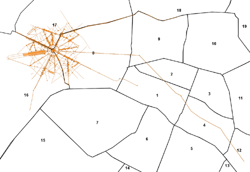
In this section, we apply what you learned in the previous section by exploring various ways to model a real city. We abandon the quadrants of D.C. and states of the United States and cross the Atlantic to Paris, the city of lights (or love, depending on your preference) for our extended example. We chose Paris because of the importance placed on arrondissements. For those of you unfamiliar with Paris, the city is divided into 20 administrative districts, known as arrondissements. Unlike people in other major cities, Parisians are keenly aware of the presence of administrative districts. It’s not unusual for someone to say that they live in the nth arrondissement, fully expecting their fellow Parisians to know perfectly what general area of Paris is being spoken of. Unlike what are often referred to as neighborhoods in other major cities, arrondissements are well defined geographically and so are well suited for GIS purposes. It’s not often that the exact geographical subdivision of a city has crept into the common usage of its citizenry. On top of it all, Parisians often refer to them by their ordinal number rather than their ascribed French names, making numerically minded folk like us extra happy.
The basic Paris arrondissements geography is illustrated in figure 3.1.
Figure 3.1. Paris arrondissements

The arrondissement arrangement is interesting in that it spirals from the center of Paris and moves clockwise around, reflecting the pattern of growth since the 1800s as the city annexed adjacent areas.
We downloaded our Paris data from GeoCommons.com as well as OpenStreetMap (OSM). We transformed all the data to SRID 32631 (WGS 84 UTM Zone 31). All of Paris fits into this UTM zone. Because UTM is meter based, we have measurements at our disposal without any additional effort. As a starting point, we model each arrondissement as a multipolygon and inserted all of them into a table called arrondissements. The table contains exactly 20 rows. Not only will this table serve as our base layer, but we’ll also use it to geo-tag additional data into specific arrondissements.
3.2.1. Modeling using a heterogeneous geometry column
If we mainly need to query our data by arrondissements without regard to the type of feature, we can employ a single geometry column to store all of our data. Let’s create this table:
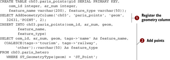
CREATE TABLE ch03.paris_hetero(gid serial NOT NULL,
osm_id integer, geom geometry,
   ar_num integer, tags hstore,
  CONSTRAINT paris_hetero_pk PRIMARY KEY (gid),
  CONSTRAINT enforce_dims_geom CHECK (st_ndims(geom) = 2),
  CONSTRAINT enforce_srid_geom CHECK (st_srid(geom) = 32631)
);
Notice how a constraint restricting the type of geometry is decidedly missing. Our geometry column will be able to contain points, linestrings, polygons, multigeometries, geometry collections—in short, any geometry type we want to stuff in. We did take the extra step to limit our column to only two-dimensional geometries and SRID of 32631.
You’ll also notice a data type called hstore. Hstore is a data type for storing key-value pairs similar in concept to PHP associative arrays. Much like geometry columns, it too can be indexed using the GIST index. OSM makes wide use of tags, for storing properties of features that don’t fit elsewhere. To bring in the OSM data without complicating our table, we used the OSM2PGSQL utility with the --hstore switch to map the OSM tags to an hstore column.
The hstore data type is a contrib module found in PostgreSQL 8.2 and above. To enable this module, execute the hstore.sql script in the share/contrib folder. In PostgreSQL 9.0+, this data type has been enhanced to allow DISTINCT and GROUP BY operations and also to support storing larger amounts of data per field.
Our table includes a column called ar_num for holding the arrondissement number of the feature. Unfortunately, this attribute isn’t one maintained by OSM. No worries, we intersect the OSM data with our arrondissement table to figure out which arrondissement each OSM record fall into. Though we can determine the arrondissements on the fly, having the arrondissements figured out beforehand means we can query against an integer instead of having to constantly perform spatial intersections later on.
Listing 3.2 demonstrates how to intersect arrondissements with OSM data to yield an ar_num value.
Figure 3.2. Our dataset overlaid on the arrondissements without caring about geometry type
Listing 3.2. Region tagging and clipping data to a specific arrondissement
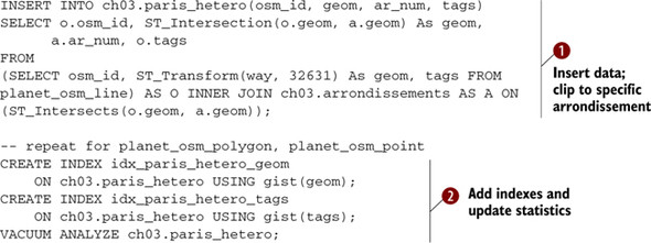
In ![]() we load in all the OSM data we downloaded. We listed only the insert from the planet_osm_line table, but you’ll need to repeat
this for OSM points and OSM polygons. Easier yet, download the code. Features such as long linestrings and large polygons
will straddle multiple arrondissements, but our intersection operation will clip them so you end up with one record per arrondissement.
For example, the famous Boulevard Saint-Germain passes through the fifth, sixth, and seventh arrondissements. After our clipping exercise, our record
with a single linestring would have been broken up into three records, each with shorter linestrings, one for each of the
arrondissements that it passes through. c We perform our usual index and update statistics after the bulk load.
we load in all the OSM data we downloaded. We listed only the insert from the planet_osm_line table, but you’ll need to repeat
this for OSM points and OSM polygons. Easier yet, download the code. Features such as long linestrings and large polygons
will straddle multiple arrondissements, but our intersection operation will clip them so you end up with one record per arrondissement.
For example, the famous Boulevard Saint-Germain passes through the fifth, sixth, and seventh arrondissements. After our clipping exercise, our record
with a single linestring would have been broken up into three records, each with shorter linestrings, one for each of the
arrondissements that it passes through. c We perform our usual index and update statistics after the bulk load.
As we’ve demonstrated, by not putting a geometry type constraint on our geometry column, we can stuff linestrings, polygons, points, and even geometry collections if we want to in the same table. This model is nice and simple in the sense that if we wanted for mapping or statistical purposes to pick all features or count all features that fit in a particular user-defined area, we could do it with one simple query. Here’s an example that counts the number of features within each arrondissement:
SELECT ar_num, COUNT(DISTINCT osm_id) As compte
FROM ch03.paris_hetero
GROUP BY ar_num;
This yields the following answer:
| ar_num | compte |
| 1 | 8 |
| : | |
| 8 | 334 |
| : | |
| 16 | 302 |
| 17 | 328 |
| 18 | 8 |
We should mention that for our example, we extracted from OSM only the area of Paris surrounding the Arc de Triomphe. The famous landmark is at the center of arrondissements 8, 16, and 17; hence, most of our features tend to be in those three regions. Figure 3.2 shows a quick map we generated in OpenJUMP by overlaying our OSM dataset atop the arrondissement polygons.
The main advantage of using hstore to hold miscellaneous attribute data is that you don’t have to set up bona fide columns for attributes that could be of little use later on just so you can import data. You can first import the data and then cherry-pick which attributes you’d like to promote to columns as your needs grow. Using hstore also means that you can add and remove attributes without fussing with the data structure. The drawback is when you do need attributes to be full-fledged columns. You can’t query inside an hstore column as easily as you can a character or numeric column or enforce numeric and other data type constraints on the hstore values. Also remember that hstore is a PostgreSQL data type, not to be found elsewhere. Few mapping tools will accept columns in hstore natively. A simple way to overcome the drawback of hstore columns is to create a view that will map attributes within an hstore column into virtual data columns, as shown here:
CREATE OR REPLACE VIEW ch03.vw_paris_points AS
SELECT gid, osm_id, ar_num, geom,
    tags->'name' As place_name,
    tags->'tourism' As tourist_attraction
FROM ch03.paris_hetero
WHERE ST_GeometryType(geom) = 'ST_Point';
In this snippet, we create a view that promotes the two tags, name and tourism, into two text data columns. Don’t forget that you can register views in the geometry_ columns table just as you can with tables. Use the handy populate_geometry_columns function to perform the registration:
SELECT populate_geometry_columns('ch03.vw_paris_points'),
Once it’s registered, we challenge any third-party program to treat the view any differently than a regular data table, at least as far as reading the data goes. Now we move on to the homogeneous architecture.
3.2.2. Modeling using homogeneous geometry columns
With the homogeneous columns approach, we want to store each geometry type in its own column or table, as shown in listing 3.3. This style of storage is more common than the heterogeneous approach. It’s the one most supported by third-party tools. Having distinct columns or tables by geometry type allows you to enforce geometry type constraints, preventing different geometry data types from inadvertently mixing. The downside is that your queries will have to enumerate across multiple columns or tables should you ever wish to pull data of different geometry types.
Listing 3.3. Breaking our data into separate tables with homogeneous geometry columns
We start by creating a table to store point geometry types. ![]() We register the geometry column, effectively constraining the column to store only points. Having a geometry type constraint
is the essence of the homogeneous approach.
We register the geometry column, effectively constraining the column to store only points. Having a geometry type constraint
is the essence of the homogeneous approach. ![]() Finally, we perform the insert, but instead of starting from the OSM data, we take advantage of the fact that we already
have the data we need in the paris_hetero table, and we selectively pick out the tags we care about and morph them into the
columns we want. If we wanted to have a complete homogeneous solution, we’d create similar tables for paris_polygons and paris_linestrings.
Finally, we perform the insert, but instead of starting from the OSM data, we take advantage of the fact that we already
have the data we need in the paris_hetero table, and we selectively pick out the tags we care about and morph them into the
columns we want. If we wanted to have a complete homogeneous solution, we’d create similar tables for paris_polygons and paris_linestrings.
If we were to get the counts of all the features by arrondissement, our query would require unioning all the different tables together, as shown here:
SELECT ar_num, COUNT(DISTINCT osm_id) As compte FROM
(SELECT ar_num, osm_id FROM paris_points
UNION ALL
SELECT ar_num, osm_id FROM paris_polygons
UNON ALL
SELECT ar_num, osm_id FROM paris_linestrings
) As X
GROUP BY ar_num;
When performing union operations you generally want to use UNION ALL rather than UNION. UNION has an implicit DISTINCT clause built in, which automatically eliminates duplicate rows. If you know that the sets you’re unioning can’t or need not be deduped in the process, opt for UNION ALL. It will be faster for sure.
We move next to an inheritance-based storage design where you’ll see that by expending some extra effort, you’ll reap the benefits of both the heterogeneous and homogeneous approaches.
3.2.3. Modeling using inheritance
Table inheritance is a feature that’s fairly unique to PostgreSQL. We gave you a quick overview in section 3.1.3. Now we’ll apply it to our Paris example. We begin by creating an abstract parent table to store attributes that all of its children will share, as shown in the following code:
CREATE TABLE ch03.paris(gid SERIAL PRIMARY KEY, osm_id integer, ar_num
     integer, feature_name varchar(200), feature_type varchar(50), geom
     geometry);

ALTER TABLE ch03.paris
ADD CONSTRAINT enforce_dims_geom CHECK (st_ndims(geom) = 2);
ALTER TABLE ch03.paris
ADD CONSTRAINT enforce_srid_geom CHECK (st_srid(geom) = 32631);
We went to the extra effort of adding a primary key on the parent table even though we never plan to add data to it. Child tables also can’t inherit primary keys, so why did we take the extra step? Besides the good practice of having a primary key on every table, abstract or not, many clients tools rely on all tables having a primary key.
With our parent table in place, we create child tables. Keep in mind that you’ll need to do this for paris_points and paris_linestrings or any other geometry type you have data for, but for the sake of brevity we’ll create only the child table for storing polygons, as shown in the next listing.
Listing 3.4. Creating a child table
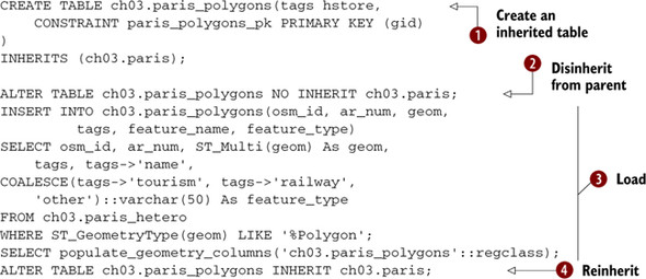
In ![]() we create a polygon table and declare it as inheriting from our paris table; we need only add the additional columns (in
this case tags) beyond what are already defined in the parent. We also add a primary key to the child table because primary
keys don’t automatically inherit. In
we create a polygon table and declare it as inheriting from our paris table; we need only add the additional columns (in
this case tags) beyond what are already defined in the parent. We also add a primary key to the child table because primary
keys don’t automatically inherit. In ![]() we disinherit the child from the parent. Disinheriting doesn’t remove inherited columns. Once a child table inherits from
a parent table, the structure of the parent is passed down permanently. The disinheritance disengages the child from the parent
so that queries against the parent don’t drill down to the children. We find it a good idea to disinherit a child table prior
to performing large bulk loads on the child table. This is to prevent someone from querying a child table while it’s in the
process of being loaded. In
we disinherit the child from the parent. Disinheriting doesn’t remove inherited columns. Once a child table inherits from
a parent table, the structure of the parent is passed down permanently. The disinheritance disengages the child from the parent
so that queries against the parent don’t drill down to the children. We find it a good idea to disinherit a child table prior
to performing large bulk loads on the child table. This is to prevent someone from querying a child table while it’s in the
process of being loaded. In ![]() , we then load our table taking rows from our paris_hetero table where the geometry type is polygon or multipolygon. We finish
up by calling the populate_geometry_columns function to automatically add the geometry constraint and register our geometry
column, and then in
, we then load our table taking rows from our paris_hetero table where the geometry type is polygon or multipolygon. We finish
up by calling the populate_geometry_columns function to automatically add the geometry constraint and register our geometry
column, and then in ![]() we reinherit from the parent.
we reinherit from the parent.
In listing 3.5 we’ll repeat the same code for linestrings, but we’ll omit the loading of data and the adding of the tag column. Because we aren’t populating the table immediately, we constrain the geometry column to store only linestrings so that our populate_geometry_columns function can use this check constraint to properly register the geometry column.
Listing 3.5. Adding another child and additional constraints

As we did with polygons ![]() we create a table that inherits from paris to store our line-strings. We aren’t ready to load data yet, but we want to constrain
the table to just line-strings, so in
we create a table that inherits from paris to store our line-strings. We aren’t ready to load data yet, but we want to constrain
the table to just line-strings, so in ![]() we add a geometry type constraint. We don’t need to add a dimension or srid constraint, because check constraints are always
inherited from the parent tables and paris already has those constraints defined. Because we have a geometry constraint,
we add a geometry type constraint. We don’t need to add a dimension or srid constraint, because check constraints are always
inherited from the parent tables and paris already has those constraints defined. Because we have a geometry constraint, ![]() the populate_geometry_columns will use the geometry constraint type to correctly register the table in geometry_columns.
the populate_geometry_columns will use the geometry constraint type to correctly register the table in geometry_columns.
At last, we reap the fruits of our labor. With inheritance our count query is identical to the simple one we used for our heterogeneous model:
SELECT ar_num, COUNT(DISTINCT osm_id) As compte
FROM ch03.paris
GROUP BY ar_num;
With inheritance in place, we have the added flexibility to query just the polygon table should we care about only the counts there:
SELECT ar_num, COUNT(DISTINCT osm_id) As compte
FROM ch03.paris_polygons
GROUP BY ar_num;
As you can see, inheritance requires an extra step or two to set up properly, but the advantage is that we’re able to keep our queries simple by judiciously querying against the parent table or one of the child tables. As one famous Parisienne might have said, “Let them have their cake and eat it too.”
Adoption
More often than not, inheritance comes as an afterthought rather than as part of the initial table design. As an example, say we already set up a paris_points table to store point geometry and have gone to great lengths to populate the table with data. We wouldn’t want to drop our points table and re-create it in order for it be a legitimate child of the paris table. In the following listing we demonstrate how to make an existing table a child of paris.
Listing 3.6. Adopt an orphan

There are a few considerations when a parent “adopts” a new child table. Before being adopted, the child table must first
ensure that its set of columns is a superset of the columns found in the parent’s table. The new parent must not have any
columns not found in the child. Though it’s not an absolute necessity, it’s useful for all children’s primary keys to be unique
across the hierarchy. One way to ensure that is to make them use the same sequence as the parent, a family genetic sequence
so to speak. To reassign the gid of our points table to use the family sequence, we drop the gid columns entirely as in ![]() . Next, we add the column back, except this time we specify that the sequence must come from the sequence of the parent; see
. Next, we add the column back, except this time we specify that the sequence must come from the sequence of the parent; see
![]() . In
. In ![]() , we make paris_points a child of paris. Finally in
, we make paris_points a child of paris. Finally in ![]() , we add a spatial index for good measure. If you’re doing bulk loads, you may wish to add the index afterwards, not before,
so the loading can run as fast as possible.
, we add a spatial index for good measure. If you’re doing bulk loads, you may wish to add the index afterwards, not before,
so the loading can run as fast as possible.
Adding Columns to the Parent
When you add a new column to the parent table, PostgreSQL will automatically add the column to all inherited children. If the child table already has that column, PostgreSQL issues a gentle warning. In our earlier example, we created our paris_polygons table with a tags column, but the parent table and none of the other child tables have this column. Let’s try adding tags to the paris table:
ALTER TABLE ch03.paris ADD COLUMN tags hstore;
When we do this, we’ll get a notice:
merging definition of column "tags" for child "paris_polygons"
This informs us that the child paris_polygons already has this column. And remember how we purposely omitted the tags column when creating the paris_linestrings child table? After adding tags to the parent, our paris_linestrings now also has this column. Check for yourself.
In the next section, we cover the use of rules and triggers. Though these two database utilities can be used wherever the situation calls for them, we find that they’re invaluable in working with inheritance hierarchies.
3.3. Using rules and triggers
Sophisticated RDBMS usually offer ways to catch the execution of certain SQL commands on a table or view and allow some form of conditional processing to take place in response to these events. PostgreSQL is certainly not devoid of such features and can perform additional processing when it encounters the four core SQL commands of SELECT, UPDATE, INSERT, and DELETE. The two mechanisms for handling the conditional processing are rules and triggers.
At this point, we count on you to have worked through the example and have in your test database the four tables paris, paris_points, paris_linestrings, and paris_ polygons. We’ll enhance our Paris example by adding in rules and triggers.
3.3.1. Rules versus triggers
Though both rules and triggers respond to events, this is where their similarity ends. They do overlap in functionality. You could often use a trigger instead of a rule and vice versa, but they were created with different intents. Though there are no steadfast guidelines on when to use one over the other when you have a choice, the underlying motivation behind having two separate event-response mechanisms will help you decide.
Rules
A rule in PostgreSQL is an instruction of how to rewrite an SQL statement. For this reason people sometimes refer to rules as rewrite rules. A rule is completely passive and only transforms one SQL statement into another SQL statement, nothing more. Unbeknownst to many people, views are nothing more than one or more rewrite rules nicely packaged together. When you execute a SELECT command from a view, the view portion of your SQL statement is rewritten to include the view definition before the command is run. For example, suppose you create a view as follows:
CREATE OR REPLACE view some_view AS SELECT * FROM some_table
When you then select from the view using a simple statement like
SELECT * FROM some_view
the rule rewriter substitutes the some_view part of the SELECT with the definition you used to create the view so that your SELECT is rewritten to be something along the lines of
SELECT * FROM (SELECT * FROM some_table) AS some_view
Because a view is nothing more than a packaging of rewrite rules, you’re free to use views far beyond a simple SELECT statement. You can have your views manipulate data. You’re free to use UPDATE, INSERT, and DELETE commands at will within your view rules. Furthermore, a view need not have just one SQL statement but can process an entire chain of statements combining SELECT, UPDATE, INSERT, and DELETE statements. Calling it a view in PostgreSQL belies its underlying capability to do much more than view data.
Triggers
A trigger is a piece of procedural code that either
- prevents something from happening, for example, canceling an INSERT, UPDATE, or DELETE if certain conditions aren’t met;
- does something instead of the requested INSERT, UPDATE, or DELETE; or
- does something else in addition to the INSERT, UPDATE, or DELETE command.
Triggers from rules can never be applied to SELECT events.
Triggers are either row based or statement based. Row-based triggers are executed for each row participating in an UPDATE, INSERT, or DELETE operation. Statement-based triggers are rarely used except for statement-logging purposes, so we won’t cover them here.
PostgreSQL 9.0 introduces a WHEN clause, which allows a trigger to be skipped if it doesn’t satisfy a designated condition. This improves the performance of triggers, because the trigger function is never entered unless the triggering data satisfies the WHEN clause.
In PostgreSQL, you have many language choices for writing triggers, but unlike with rules, you can’t simply string together a series of SQL statements. Triggers must be standalone functions. Popular languages for authoring functions in PostgreSQL are PL/PGSQL, PL/Python, PL/R, PL/TCL, and C. You could even develop your own language should you fancy to do so or have multiple triggers on a table each written in a different language more suited for a particular task.
When to use Rules, When to use Triggers
Broadly speaking, triggers are more powerful but must be executed for each row. For bulk loads, rules can often be faster because they’re called once per UPDATE or INSERT statement, whereas triggers are called for each row needing an UPDATE or INSERT. In situations where only a few rows are involved, the speed difference between rules and triggers is negligible.
In certain situations only rules can be used. Should you need to bind to a view, only rules will work for versions of PostgreSQL prior to PostgreSQL 9.1.
In PostgreSQL 9.1, one of the features introduced is the ability to define an instead of trigger on a view to more closely follow the ANSI SQL:2003 standard. Example of usage can be found in http://www.depesz.com/index.php/2010/10/16/waiting-for-9-1-triggers-on-views/.
Then there are situations when you can’t use a rule and have to implement a trigger. Should you need the logic or specialized functions of procedural languages, these are available only through triggers. Rules are always written in plain SQL. You’d also need a trigger if you needed to execute SQL commands such as CREATE, ALTER, or DROP. You can’t run Data Definition Language statements with rules. You also don’t have the facilities within rules to build SQL statements on the fly.
Here are some general heuristics we follow: Use rules when
- Creating a select-only view
- Making a view updateable
- Doing bulk loads
- Binding to views
Use triggers when
- Redirecting inserts from parent tables to child tables
- Preprocessing logic such as converting lon lat to geometry/geographies or geo-tagging data
- Doing complex validation or with procedural languages
- Needing to run create table or other DDL statements in response to changes in data
The most important thing to keep in mind is that despite their overlap in achieving the same goal, rules and triggers are fundamentally different. Rules rewrite an SQL statement. Triggers run a function for each affected row.
3.3.2. Using rules
Before we provide you with some example uses of rules, you need to understand the distinction between a DO rule versus a DO INSTEAD rule. The default behavior of a rule when not specified is a DO rule. A DO rule takes an SQL statement and tacks additional SQL onto the statement. A DO INSTEAD, on the other hand, throws out the original statement and replaces it with the rewritten SQL. The technical term for a query broken into subparts is query tree. With a DO rule, you add additional branches to the tree. With a DO INSTEAD rule, you supplant the tree completely with a new tree. One last thing to keep in mind is that for views, you can use only DO INSTEAD rules.
In the next listing, we’ll create a simple view and then add rules so that we can use the view to perform INSERT, UPDATE, and DELETE operations.
Listing 3.7. Making views updateable with rules
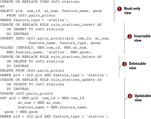
With ![]() we use a simple SELECT to define our view. At this point our view is read-only. We then define an insert rule in
we use a simple SELECT to define our view. At this point our view is read-only. We then define an insert rule in ![]() , which will allow inserts into this view. We assume that only stations will be added using this view and so deliberately
set the feature_type to ‘station’. Our insert rule replaces the original insert with the code you see in
, which will allow inserts into this view. We assume that only stations will be added using this view and so deliberately
set the feature_type to ‘station’. Our insert rule replaces the original insert with the code you see in ![]() , effectively redirecting the insert to the paris_points table. In
, effectively redirecting the insert to the paris_points table. In ![]() we create a delete rule. In addition to the primary key field, we have a filter to delete only stations. This ensures that
even if we forget a filtering WHERE clause when performing the deletion, the worst we can do is remove all station rows as
oppose to all rows or paris_points. Finally, in
we create a delete rule. In addition to the primary key field, we have a filter to delete only stations. This ensures that
even if we forget a filtering WHERE clause when performing the deletion, the worst we can do is remove all station rows as
oppose to all rows or paris_points. Finally, in ![]() , we have the update rule.
, we have the update rule.
Both rules and triggers can have available to them two record variables called NEW and OLD. For INSERT FOR EACH ROW events, only NEW is available. For DELETE FOR EACH ROW events, only OLD is available. For UPDATE FOR EACH ROW events, both NEW and OLD are available. For statement-level triggers, neither NEW nor OLD is available. Both NEW and OLD represent exactly one record and take on the column structure of the triggering table. OLD represents the record that was deleted or replaced. You can think of an UPDATE as being a combination INSERT and DELETE, which is why it has both a NEW and an OLD.
This behavior is similar to other relational databases you may have come across, except that the NEW and OLD always represent one row, whereas in some other databases the comparable counterparts are tables consisting of all the records to be inserted or deleted.
Let’s take our view for a test drive. We start with a DELETE from the view as follows:
DELETE FROM ch03.stations;
The database query engine automatically rewrites this as
DELETE FROM ch03.paris_points WHERE feature_type = 'station';
Our stations have all vanished. We next add back our stations as follows:
INSERT INTO ch03.stations(osm_id, feature_name, geom)
SELECT osm_id, tags->'name', geom
FROM ch03.paris_hetero
WHERE tags->'railway' = 'station';
With the rewrite, our insert becomes
INSERT INTO ch03.paris_points(osm_id,
       feature_name, feature_type, geom)
VALUES (NEW.osm_id, NEW.ar_num,
    NEW.feature_name, 'stations', NEW.geom)
As you can see, rules rewrite the original SQL, nothing more. During the rewrite, you’re limited to using SQL statements. This does limit the capability of rules in many situations, but for core logic that you wish to apply universally and forever, rules may fit the bill. Now we move onto triggers.
3.3.3. Using triggers
When it comes to triggers, we must expand the three core events of INSERT, UPDATE, and DELETE to six: BEFORE INSERT, AFTER INSERT, BEFORE UPDATE, AFTER UPDATE, BEFORE DELETE, and AFTER DELETE. BEFORE events fire prior to the execution of the triggering command; AFTER events fire upon completion. Should you wish to perform an alternative action as you can with a DO INSTEAD rule, you’d create a trigger and bind it to the BEFORE event but throw out the resulting record. If you need to modify data that will be inserted/updated, you also need to do this in a BEFORE event. An AFTER trigger would be too late. Similarly, should you wish to perform some operation that depends on the success of your main action, you’d need to bind to an AFTER event. Examples of this are if you need to insert or update a related table on success of an INSERT or UPDATE statement.
PostgreSQL triggers are implemented as a special type of function called a trigger function and then bound to a table event. This extra level of indirection means you can reuse the same trigger function for different events and tables. The slight inconvenience is that you face a two-step process of first defining the trigger function and then binding it to a table.
PostgreSQL allows you to define multiple triggers per event per table, but each trigger must be uniquely named across the table. Triggers fire in alphabetical sequence. If your database is trigger happy, we recommend developing a convention for naming your triggers to keep them organized.
We’ll now move on to a series of examples showcasing how you can use triggers in a variety of situations to fortify your data model. Triggers are powerful tools, and your mastery of them will allow you to develop database applications that can control business logic without need of touching the frontend application.
Redirecting Inserts with Before Triggers
For our first trigger example, we’ll demonstrate a common need when working with inherited tables. This is the ability to redirect inserts done on a parent table to the child tables. Recall that with an inheritance hierarchy with abstract parents, we want people to think they’re inserting into the parent table, but we don’t want any data going into it. To accomplish this we use a BEFORE INSERT trigger to redirect inserts into child tables. Our function checks the geometry type of the record being inserted into the table. Depending on its geometry type, we redirect the insert to one of the child tables. For geometry types that don’t fit, we toss them into a rejects table created using the following:
CREATE TABLE ch03.paris_rejects
(
  gid integer NOT NULL PRIMARY KEY,
  osm_id integer,
  ar_num integer,
  feature_name varchar(200),
  feature_type varchar(50),
  geom geometry, tags hstore);
The before insert trigger is shown in the following listing.
Listing 3.8. PL/PGSQL BEFORE INSERT trigger function to redirect insert
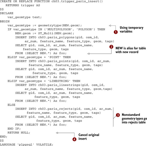
In ![]() , we declare a temporary variable to hold intermediary information. This can reduce processing time for long-running functions,
plus we end up with clearer code. During an insert operation, PostgreSQL automatically dumps the new record into a single-rowed
table, aliased NEW, with the exact structure as the table being inserted into. In
, we declare a temporary variable to hold intermediary information. This can reduce processing time for long-running functions,
plus we end up with clearer code. During an insert operation, PostgreSQL automatically dumps the new record into a single-rowed
table, aliased NEW, with the exact structure as the table being inserted into. In ![]() , we take advantage of this alias to read the values of the geometry type of the new record coming in order to decide which
child table to redirect the insert to. Normally when you finish with a BEFORE trigger, you return the new record, which you
may have changed in the trigger. This signals to the PostgreSQL to continue with the INSERT.
, we take advantage of this alias to read the values of the geometry type of the new record coming in order to decide which
child table to redirect the insert to. Normally when you finish with a BEFORE trigger, you return the new record, which you
may have changed in the trigger. This signals to the PostgreSQL to continue with the INSERT. ![]() But in our case, we want to halt the INSERT into the parent table altogether, so we return NULL instead of NEW.
But in our case, we want to halt the INSERT into the parent table altogether, so we return NULL instead of NEW. ![]() Returning the NEW record is usually used only in a BEFORE trigger, because in an AFTER trigger, there’s no hope of being
able to change the record being inserted or updated because the event has already happened. This is a common mistake people
make—defining an AFTER trigger and then trying to change the NEW record. PostgreSQL will let you do that, but the changes
will never make it into the underlying table.
Returning the NEW record is usually used only in a BEFORE trigger, because in an AFTER trigger, there’s no hope of being
able to change the record being inserted or updated because the event has already happened. This is a common mistake people
make—defining an AFTER trigger and then trying to change the NEW record. PostgreSQL will let you do that, but the changes
will never make it into the underlying table.
In trigger functions, you’ll often see the use of NEW.* as shorthand to pick up all the columns of the record being inserted. The single-row NEW not only has the same structure, but it also has the exact column order as the triggering table. This often allows you to use the following insert syntax without worrying about listing out each column:
INSERT INTO ch03.paris_rejects VALUES(NEW.*);
For our example we’ve chosen not to use this syntax. Although this syntax is extremely powerful because you can use it in any trigger function without knowing beforehand what the columns are or will be, it’s not without danger.
The danger of this approach is when you’re redirecting inserts to child tables. A child table may have more columns than its parent or in a different order, so this syntax will fail in such cases.
Remember that trigger functions do us no good unless they’re bound to a table event. To bind the previous trigger function to the BEFORE insert of our paris table, we run this statement:
CREATE TRIGGER trigger1_paris_insert BEFORE INSERT
ON ch03.paris FOR EACH ROW
EXECUTE PROCEDURE ch03.trigger_paris_insert();
Let’s take our new trigger for a test drive. Before we do, we’ll delete any data we have thus far to get a clean start. As long as we have no foreign-key constraints, we can use the fast SQL TRUNCATE clause to delete data from the parent table and all of its child tables:
TRUNCATE TABLE ch03.paris;
Now when we perform our insert,
INSERT INTO ch03.paris (osm_id, geom, tags)
SELECT osm_id, geom, tags FROM ch03.paris_hetero;
with the trigger in place, the records will sort themselves into child tables befitting their respective geometry types. Because we never created a child table for multilinestrings, these records will end up in the paris_rejects table.
Creating Tables on the Fly With Triggers
Using triggers allows us to do something we can’t do with rules. We can generate any SQL statements on the fly and execute them as part of our trigger function. We can even run SQL that will create new database objects, which is what we’ll demonstrate with our next example. Suppose, we want to partition our Paris data by arrondissements in addition to geometry type, but we’re too lazy to create all 60 arrondissement tables beforehand. We can delegate the work to our trigger function. As we insert new records into the parent table, it will redirect inserts to each geometry type child table, which in turn will redirect inserts to each geometry-arrondissement grandchild table as appropriate. Furthermore, if the particular grandchild geometry-arrondissement table doesn’t exist, our trigger function will create it.
For the few arrondissements we have or if we know the tables we need beforehand, our dynamic creation in a trigger is overkill. It’s more efficient to have the tables created at the outset than to have each insert check and then create as needed, but you could imagine cases where this may not be possible. For example, you may have a large amount of financial data that you’d like to break out into weekly tables. If you anticipate your database being in use for 10 years, you’ll have to prepare 520 tables at the start. Not only that, on the first day of the eleventh year, your database will fail. The following listing shows a trigger that creates tables as needed.
Listing 3.9. Trigger that dynamically creates tables as needed

Before we do anything, we must settle on a naming convention for all of our geometry-arrondissement grandchild tables. We
choose paris_points_ar01 through paris_ points_ar20, paris_linestrings_ar01 through paris_linestrings_ar20, and paris_ polygons_ar01
through paris_polygons_ar20. In ![]() , we formulate the destination table name of our new record. Notice how PostgreSQL provides a TG_TABLE_NAME variable that
tells us the table to which the current trigger is bound to. Without this, we’d have to further test the geometry type of
the new record to figure the destination table. In
, we formulate the destination table name of our new record. Notice how PostgreSQL provides a TG_TABLE_NAME variable that
tells us the table to which the current trigger is bound to. Without this, we’d have to further test the geometry type of
the new record to figure the destination table. In ![]() , we check to see if the destination table is present. If not, we create it in
, we check to see if the destination table is present. If not, we create it in ![]() . By
. By ![]() , we’re assured that the destination table must be present and proceed with the insert.
, we’re assured that the destination table must be present and proceed with the insert.
Once we have our trigger function, we bind it to our three child tables: paris_points, paris_linestrings, and paris_polygons, as follows.
Listing 3.10. Binding same trigger function to multiple tables
CREATE TRIGGER trig01_paris_child_insert BEFORE INSERT
    ON ch03.paris_polygons FOR EACH ROW
    EXECUTE PROCEDURE ch03.trigger_paris_child_insert();

CREATE TRIGGER trig01_paris_child_insert BEFORE INSERT
    ON ch03.paris_points FOR EACH ROW
    EXECUTE PROCEDURE ch03.trigger_paris_child_insert();

CREATE TRIGGER trig01_paris_child_insert BEFORE INSERT
    ON ch03.paris_linestrings FOR EACH ROW
    EXECUTE PROCEDURE ch03.trigger_paris_child_insert();
Once in place, these three triggers will prevent data from being inserted into our child tables but instead have the data flow to arrondissement-specific grandchild tables. If the grandchild is missing, we create it on the fly. To test our new trigger, we delete all the data we’ve inserted and start anew:
TRUNCATE TABLE ch03.paris;
TRUNCATE TABLE ch03.paris_rejects;
We then perform the insert:
INSERT INTO ch03.paris(osm_id, geom, tags, ar_num)
SELECT osm_id, geom, tags, ar_num FROM ch03.paris_hetero;
After we’ve finished, and provided we have data to fully span all three geometry types and 20 arrondissements, we should end up with 60 tables. Our particular dataset will only require the creation of 9 tables.
Before bringing the discussion of rules and triggers to an end, let’s revisit constraint exclusions. Remember how before we began our extended example, we described the usefulness of having constraint exclusion enabled? To test that constraint exclusion is working correctly, we run the following query and look at the pgAdmin graphical explain plan.
SELECT * FROM ch03.paris WHERE ar_num = 17;
The graphical explain plan output of this query is shown in figure 3.3.
Figure 3.3. Only empty parent tables and child tables holding ar17 data are searched.

Observe that although there exist tables such as paris_points_ar01, paris_polygons_ar08, and so on, the planner strategically skips over those tables because we asked only for data found in ar17 tables. Constraint exclusion works!
3.4. Summary
In this chapter we discussed some approaches you can use for storing PostGIS geometry data in PostgreSQL relational tables as well as managing control of this data. We also demonstrated the use of the PostgreSQL custom key value hstore data type for implementing schema-less models. We followed up by applying these approaches to storing Parisian data.
We demonstrated in this chapter that PostGIS geometry columns are like other columns you’ll find in relational tables. They have indexes and are stored along with other related data such as text columns. Like other data types, they take advantage of all the facilities that the database has to offer such as inheritance, triggers, rules, indexes, and so forth. In addition, you can inspect geometries using various geometry functions designed for them and can even use them in SQL join conditions as you would other relational data types.
This chapter also provided a sneak preview of some of the PostGIS functions we’ll explore in later chapters. In the next chapter and chapters that follow, we’ll explore PostGIS functions in more depth. We’ll first focus on dealing with single geometries and the more common properties, various functions you can use to inspect and modify geometries. After looking at single geometry functions, we’ll focus on functions that involve interplay between two or more geometries and geometry columns.