
Chapter 4. Geometry functions
In the previous chapters we defined the various kinds of geometries that PostGIS provides, how to create them, and how to add them to the database. In this chapter and the next we’ll introduce the core set of functions that work with geometries. This chapter will concentrate on functions that tend to work with single geometries. In the next, we’ll work with functions that relate two or more geometries.
PostGIS offers well over 300 functions and operands. To get an overview, we’ve developed a taxonomy that’s driven by intent of use. This is by no means a rigorous classification nor one that will neatly sort each function into a unique classification without ambiguities. Grouping functions by the types of tasks that we’re trying to accomplish has been the handiest approach in our experience. Before delving into the functions themselves, let’s go through our classification scheme:
- Constructor functions— Use these functions to create PostGIS geometries from either a well-known text (WKT) or a well-known binary (WKB).
- Output functions— Use these functions to output geometry representations in various well-defined standard formats (WKT, WKB, GML, SVG, KML, GeoJSON).
- Accessor and setter functions— These are functions that work against a single geometry and return or set attributes of the geometry.
- Decomposition functions— These functions extract geometries from an input geometry.
- Composition functions— Use these functions to stitch, splice, or group together geometries.
- Measurement functions— These functions return scalar measurements of a geometry.
- Simplification functions— Sometimes you don’t need the full resolution of a geometry. These functions simplify a geometry by removing points or linestrings or by rounding the coordinates. The resultant geometry will still have the basic look and feel of the original but will contain fewer points or coordinates of lower precision.
In keeping with the fundamental mission of this book, which is to show how to use PostGIS rather than serve as a reference volume, we’ll introduce a dozen functions that are commonly used. You can find an exhaustive listing of all functions and their usage in the official PostGIS manual.
You’ll notice that almost all functions start with the two letters ST. The S stands for “spatial” and the T stands for “temporal,” even though support in the temporal dimension never gained much popularity.
The ST prefix is usually set aside for SQL/MM functions in other spatial databases, but PostGIS uses the prefix both for SQL/MM and for functions unique to PostGIS.
We’ll start with constructors.
4.1. Constructors
As the name implies, constructor functions create geometries. There are two common ways to create new geometries. The first uses raw data in an acceptable format and builds the geometry from scratch. The second way is to take existing geometries and either decompose, splice, slice, dice, or morph them to form new ones. In this section, we start with the first approach. We’ll go through the list of common representations of geometric data and the functions used to transform them into bona fide PostGIS geometry objects. Following that we’ll introduce some handy functions that create new geometries from existing ones.
4.1.1. Creating geometries from well-known text and well-known binary representations
These indispensable functions will output geometries when you feed them various text or binary representations. They are especially useful for quick viewing of geometries in various desktop tools. In tools that understand only geometries, the use of these functions becomes almost perfunctory.
St_Geomfromtext
Recall from chapter 1 that a common way to represent geometries is through well-known text representations. PostGIS provides a function called ST_GeomFromText that can be used to build 2D geometries. This function is an SQL/MM standard function that can be found in other SQL/MM–compliant spatial databases. It supports only 2D because the SQL/MM–released specs for this function don’t support M and Z coordinates. Following are examples of its use:
SELECT * INTO table1
FROM ( VALUES
    ( ST_GeomFromText('POINT(-100 28)', 4326) ),
    ( ST_GeomFromText('LINESTRING(-80 28, -90 29)', 4326) ),
    ( ST_GeomFromText('POLYGON((10 28, 9 29, 7 30, 10 28))' ) ) ) As
     foo(geom);
St_Geomfromewkt
PostGIS provides another function called ST_GeomFromEWKT. This is a PostGIS-only function and accepts input from a PostGIS-only format—EWKT (extended WKT)—with the intent of making up for deficiencies in the WKT format. EWKT encodes SRID information directly into the WKT and also supports 3D and 4D geometries. We show you how to use ST_GeomFromEWKT here. Note that EWKT explicitly prepends the SRID of the geometry.
SELECT * INTO table2
FROM ( VALUES
    (ST_GeomFromEWKT('SRID=4326;POINT(-100 28)')),
    (ST_GeomFromEWKT('SRID=4326;LINESTRING(-80 28,-90 29)')),
    (ST_GeomFromEWKT('SRID=4326;POLYGON((10 28, 9 29, 7 30, 10 28))' ) ) ) As
     foo(geom);
ST_GeomFromEWKT can accept geometries in plain WKT format as well, so it’s often preferred when SQL/MM compliance isn’t a concern.
St_Geomfromwkb and St_Geomfromewkb
On many occasions, you’ll find yourself needing to import data from a client application where geometries are already stored in binary representations. This is where the functions ST_GeomFromWKB and ST_GeomFromEWKB come into play. Again, ST_GeomFromWKB is an SQL/MM–defined function, and ST_GeomFromEWKB is a PostGIS extension offering SRID encoding and support for 3D and 4D geometries. These two functions accept byte arrays instead of text strings. One advantage of byte arrays is that they’re exact, whereas the ST_GeomFromText and ST_GeomFromEWKT functions truncate at about the fifteenth digit after the decimal point. Following is an example of using ST_GeomFromWKB:
SELECT
     ST_GeomFromWKB(E'\001\001\000\000\000\321\256B\312O\304Q\300\
     347\030\220\275\336%E@',4326);
Observe that if you were to output the well-known binary of this function,
SELECT
ST_AsBinary(ST_GeomFromWKB(E'\001\001\000\000\000\321\256B\312O\304Q
     \300\347\030\220\275\336%E@',4326));
it would look like this in pre-PostgreSQL 9.0, but it may look different in newer versions depending on your PostgreSQL bytea_output setting:
�01�01�00�00�00321256B312O304Q300347�30220275336%E@
The extra slashes we put in when feeding in the value are to escape out the “” in the string. This is needed only if your database has standard_conforming_strings=off, which is the default for PostgreSQL versions older than PostgreSQL 9.0.
Following is an example if you have standard_conforming_strings=on:
set standard_conforming_strings = on;
SELECT
ST_GeomFromWKB('�01�01�00�00�00321256B312O304Q300347�302202753
36%E@'),
Try doing a simple select statement from a geometry column, unadorned with any functions, and you’ll end up with something that looks like a long string of digits. This is actually a hexadecimal representation of the EWKB notation. You can create a geometry with this canonical form by doing the ANSI SQL compliant
SELECT CAST('0101000020E61000008048BF7D1D2059C017B7D100DEB23C40'
As geometry);
or the PostgreSQL short cast notation
SELECT '0101000020E61000008048BF7D1D2059C017B7D100DEB23C40'::geometry;
To be in conformance with OGC-MM, PostGIS offers other functions such as ST_PointFromText, ST_PolyFromText, ST_GeometryFromText, and so on. Our advice, as far as using PostGIS is concerned, is to stay away from them and stick with ST_GeomFromText, ST_Point, ST_MakePoint, ST_GeomFromWKB, and the like. The reason for that is that these other functions are just wrappers around ST_GeomFromText, with a check to make sure that the geometry is actually a polygon, point, or other type and to nullify it if it isn’t. There’s no need for such checking if your tables are set up correctly and accept only specific geometry types. These extra functions add unnecessary overhead to your inserts and updates.
4.1.2. Autocasting in PostgreSQL/PostGIS
You’ll encounter instances where someone might take a text representation of a geometry and uses it as a parameter to a function. Although this is convenient, you should exercise caution when you do this. Here’s a demonstration of such a practice:
SELECT ST_Centroid('LINESTRING(1 2,3 4)'),
To see the output, we do this:
SELECT ST_AsText(ST_Centroid('LINESTRING(1 2,3 4)'));
which returns this:
POINT(2 3)
This practice makes you forget that a centroid works on a geometry, not a string. It works because an autocast is built into PostGIS that takes a string and converts it to a geometry automatically. The more verbose but clearer way to write the statement is as follows:
SELECT ST_Centroid(ST_GeomFromText('LINESTRING(1 2,3 4)'));
A problem can arise, however, when you have two functions that take different data types and both data types have an autocast built in. In that case you could end up with an ambiguity error. Here’s a classic example:
SELECT ST_Box3D('BOX(1 2, 3 4)'),
PostgreSQL will throw a casting error because ST_Box3D can accept both a box object and a geometry, but after autocasting the text representation to a geometry, PostgreSQL no longer knows whether you intended to pass in a box or a geometry. Here’s another example that will fail. ST_XMin is a function defined only for Box3D. This one will fail because there is no autocast that will convert a text representation of a geometry directly into a Box3D, although there is one that takes a text representation of a Box2D to a Box3D:
SELECT ST_XMin('LINESTRING(1 2, 3 4)'),
PostgreSQL throws the following error:
ERROR: BOX3D parser - does not start with BOX3D;
Bypass the autocasting with the following query:
SELECT ST_XMin('LINESTRING(1 2, 3 4)'::geometry::box3d);
In the next section we’ll discuss output functions, which are the opposite of input functions. PostGIS offers a lot more output functions than input functions to accommodate the ever-growing number of GIS client tools requesting their data in a particular format.
4.2. Outputs
Output functions are functions that return a geometry representation in another industry-standard format. This allows third-party rendering tools with no knowledge of PostGIS to be repurposed and used as a display tool for PostGIS.
In this section we’ll summarize the output formats available, give general use scenarios, and discuss the PostGIS functions to output them. We’ll cover some of the more popular output formats, but you should check the official PostGIS site for the ever-growing list. To learn more about the various output format themselves, be sure to visit their own sites. We won’t go into detail about the various formats.
Finally, we advise that you use good judgment rather than memorize the intricacies of each function when it comes to determining whether the output makes sense for your particular geometry types. For example, if you have only known a particular format to support 2D with SRID 4326, make sure your geometries are all 2D with SRID 4326 prior to using the export function instead of trying your luck. This will save you time from having to remember how each function handles exceptions and will make sure your code still works should the default handling of the output functions change, as they often do with each version of PostGIS.
4.2.1. Well-known text and well-known binary
Well-known text is the most common OGC standard format for geometries. We’ve already used this format quite extensively in the book to show the output of queries because it provides a clear text representation of the underlying geometry.
Two functions that output geometries in this format are ST_AsText and ST_AsEWKT. Recall from earlier discussions that the ST_AsEWKT function is a PostGIS-specific extension loosely based on the OGC-MM WKT standard, but it isn’t considered OGC compliant. The OGC-compliant function is ST_AsText, but this function won’t output the SRID or the M or Z coordinate. This could change in the future because draft MM standards already propose the addition. Finally, textual representation will always lack the precision of binary representation and will preserve only about 15 significant digits.
Well-known binary is an OGC standard format. Two functions that output geometries in this format are ST_AsBinary and ST_AsEWKB. The ST_AsEWKB function is a PostGIS-specific extension loosely based on the standard, but it’s not OGC compliant. ST_AsBinary won’t output the SRID or the M or Z coordinate, but ST_AsEWKB will. Unlike text representation, binary format maintains precision. You can be assured that what is stored in your database is what you’re outputting, and that what you export can be read back into the database with the inverse functions ST_GeomFromWKB and ST_GeomFromEWKB.
4.2.2. Keyhole Markup Language
Keyhole Markup Language (KML) is an XML-based format created by the Keyhole Corporation to render its applications. KML gained enormous popularity after Google acquired Keyhole and integrated KML into its own mapping offerings of Google Maps and Google Earth. OGC has recently accepted KML as a standard transport format in its own right.
The PostGIS function for exporting to KML is ST_AsKML. As of PostGIS 1.4, there are four variants of this function. The default outputs in KML version 2 with 15-digit precision. Other variants allow you to change the target KML version and precision.
The spatial reference system for KML is WGS-84 lon lat (SRID 4326). As long as your geometry is in a known SRID (via membership in the spatial_ref_sys metatable), ST_AsKML functions will automatically convert it to SRID 4326 for you.
ST_AsKML supports both 2D and 3D geometries but will throw an error in PostGIS 1.4 and above when exporting curved geometry or geometry collections. Prior versions of PostGIS return NUL for unsupported geometry types. Also keep in mind that although the ST_AsKML functions will accept geometries containing an M coordinate, they won’t output the M coordinate.
4.2.3. Geography Markup Language
Geography Markup Language (GML) is an XML-based format and an OGC-defined transport format. It’s commonly used in Web Feature Services (WFS) to output the columns of a query.
The PostGIS function for exporting to GML is ST_AsGML. As of PostGIS 1.4, five variants of this function allow you to vary the target GML versions and precisions. Supported GML versions are 2.1.2 (pass in as 2) and 3.1.1 (pass in as 3). If no version parameter is passed in, then 2.1.2 is assumed. Two additional parameters control the number of significant digits and a bit field indicating whether to use short CRS (Coordinate Reference Systems).
ST_AsGML supports 2D and 3D for both geometries and geometry collections. If a geometry has an M coordinate, the M is dropped. Passing in curved geometries will throw an error in PostGIS versions 1.4 and above and return NULL in older versions.
4.2.4. Geometry JavaScript Object Notation
Geometry JavaScript Object Notation (GeoJSON) is a recently developed format based on JavaScript Object Notation (JSON). GeoJSON is geared toward consumption by Ajax-oriented applications (such as OpenLayers) because its output notation is in JavaScript format. JSON is the standard object representation in JavaScript data structures. GeoJSON extends JSON by defining a format for geometry storage within the JSON format. More detail on GeoJSON specification can be found here: http://geojson.org/geojson-spec.html.
The PostGIS function for exporting to GML is ST_AsGeoJSON (first introduced in PostGIS 1.3.5). There are six variants of this function as of PostGIS 1.5. The arguments are similar to those for ST_AsGML–target version, number of decimal places, and an encoded flag denoting whether to include the bounding box, short or long CRS, and other options. ST_AsGeoJSON supports 2D and 3D and geometry collections. It will drop the M coordinate and throw an error for curved geometries.
4.2.5. Scalable Vector Graphics
Scalable Vector Graphics (SVG) has been around for a while and is popular among high-end rendering tools as well as drawing tools such as Inkscape. Toolkits such as ImageMagick can easily convert SVG to many other image formats. It’s also one of the basic formats used by Macromedia Flash/Flex. Microsoft Silverlight’s XAML also uses a derivative of the basic SVG format. Most web browsers support it, either natively or via an installable plug-in.
The PostGIS function for exporting to SVG is ST_AsSVG. As of PostGIS 1.4, this function outputs only 2D geometries without SRIDs or Z or M coordinates and also doesn’t output curved geometries. Three variants of the function indicate whether the output points are relative to an origin or relative to the coordinate system and indicate the level of precision desired.
4.2.6. Geohash
Geohash is a lossy geocoding system for longitudes and latitudes. It’s meant more as a tool for the easy exchange of coordinates than for visual presentation. You can explore its details at http://geohash.org.
PostGIS outputs to Geohash via the ST_Geohash function. Naturally, ST_GeoHash always outputs lon lat (WGS 84) coordinates. Your data must have a known SRID so that ST_GeoHash can automatically transform it for you. ST_GeoHash can support curved geometries but ignores their Z and M coordinates. Keep in mind that Geohash is point based, so if you output anything other than points, ST_GeoHash will output only an interpolated point within the bounding box. If you use it to output an area that’s too big, it will refuse to proceed.
4.2.7. Examples of output functions
It’s now time to present a grand example that brings all the output functions together. We’ll be asking our functions to output a line string in SRID 4326 to a precision of five significant digits. (The linestring originates in northern France and terminates in southern England.)
SELECT ST_AsGML(geom,5) as GML, ST_AsKML(geom,5) As KML, ST_AsGeoJSON(geom,5)
     As GeoJSON, ST_AsSVG(geom,0,5) As SVG_Absolute, ST_AsSVG(geom,1,5) As
     SVG_Relative, ST_GeoHash(geom) As Geohash
FROM (SELECT ST_GeomFromText('LINESTRING(2 48, 0 51)', 4326) As geom) foo;
The results are shown in table 4.1.
Table 4.1. Results of the preceding code
|
Format |
Output |
|---|---|
| GML | <gml:LineString srsName="EPSG:4326"><gml:coordinates>-2,48 1,51</gml:coordinates></gml:LineString> |
| KML | <LineString><coordinates>2,48 1,51</coordinates></LineString> |
| GeoJSON | {"type":"LineString","coordinates":[[2,48],[1,51]]} |
| SVG_Absolute | M 2 -48 L 1 -51 |
| SVG_Relative | M 2 4 L -1 -3 |
| Geohash | u |
Before moving on to the next section, remember that the output functions we covered export only the geometry fragments necessary to create a fully functional data value in the various formats. Many formats have associated scalar attribute data, but the PostGIS functions will ignore these. For example, KML and JSON often embed scalar data within JSONed and KMLed wrappers, and these will be lost in translation. In the next section, we’ll cover the scalar setter and accessor functions that will be useful for exchanging the non-geometric aspects of geometries.
4.3. Accessor functions: getters and setters
If you’re experienced with any object-oriented language, accessor functions come as nothing new. The term comes from OO programming to mean any function that gets or sets intrinsic properties of a geometry. Because quite a large number of functions fall under this classification, we decided to use the term only for functions that return entities that aren’t geometries. For example, if we have a square polygon, we’d consider functions that return or set the type, the SRID, and dimension to be accessors. Functions that return the centroid (a point), the diagonal (linestring), or the boundary (linestring collection) we’ll call decomposition functions and save for a later section. We also don’t consider measurement functions such as those for computing length, area, and perimeter as getters.
A few defining characteristics of geometries are important to know when you’re using spatial accessor functions:
- Spatial reference system (SRS) defines the spatial coordinate system, ellipsoid/ spheroid, and the datum of the coordinates used in defining the geometry.
- Geometry type defines the kind of geometry: a point, linestring, polygon, multi-polygon, multicurve, and so on.
- Coordinate dimension is the dimension of the vector space in which our geometry lives. In PostGIS, this can be 2, 3, or 4.
- Geometric dimension is the minimal dimension of the vector space necessary to fully contain the geometry. (There are many more rigorous definitions, but we stick with something intuitive.) In PostGIS, geometry dimensions can be 0 (points), 1 (linestrings), or 2 (polygons).
In this section, we go into detail about these intrinsic properties of geometries and the various functions to get and set them.
4.3.1. Getting and setting spatial reference system
For every locational application involving measurements, the concept of a spatial reference system and the choice of the appropriate base spatial reference system are of utmost importance. Spatial reference systems allow meaningful measurements and make it possible to share data.
In PostGIS, ST_SRID retrieves the spatial reference system of a geometry. You’ll find this OGC SQL/MM standard function in most spatial databases. The companion setter function is ST_SetSRID(), also an SQL/MM standard. This setter function will replace the spatial reference metadata embedded within a geometry. Remember that all geometries must have an SRID, even if it’s the unknown SRID (-1). Let’s take a look at uses of this accessor in the following listing:
Listing 4.1. Example use of ST_SRID

If you set up your production tables properly, your geometries should contain only SRIDs found in the spatial_ref_sys metatable. Although nothing in the OGC specification requires SRIDs to have any real-world significance, PostGIS prepopulates the spatial_ ref_sys metatable with only the EPSG-approved SRIDs. You’re free to invent your own SRIDs and add them to the metatable. People commonly add SRIDs defined by ESRI because PostGIS databases are often used to export, import, or directly service ESRI tools.
4.3.2. Transform to a different spatial reference
No discussion of spatial reference can be complete without introducing the ST_Transform function, which converts all the points of a given geometry to coordinates in a different spatial reference system. A common application of this function is to take a WGS 84 lon lat geometry and transform it to a planar spatial reference system so that you can take meaningful measurements of the geometry of interest. Following is an example that takes a road in somewhere in New York State expressed in WGS 84 lon lat and converts it to WGS 84 UTM Zone 18N meters:
SELECT ST_AsEWKT(ST_Transform(ST_GeomFromEWKT('SRID=4326;
           LINESTRING(-73 41, -72 42)'), 32618));
The output of this code snippet is
SRID=32618;LINESTRING(668207.88519421 4540683.52927698,
       748464.920715711 4654130.89132385)
Now that we’ve transformed from geodetic measure to planar measure, obtaining the length is nothing more than a simple application of the Pythagorean theorem.
People often get confused between ST_SetSRID and ST_Transform functions. You must remember that ST_SetSRID doesn’t change the coordinates of a geometry. It simply adds information to the header of the geometry stating that its frame of reference is a particular spatial reference. ST_SetSRID comes in useful when you realize that you made a mistake during import of data. For example, if you import your geometries as WGS 84 lon lat (SRID 4326), and you later realize they were defined using NAD 27 lon lat coordinates (SRID 4267), ST_SetSRID will correct the mistake.
The ST_Transform function changes the coordinates of each point of a geometry from the geometry’s stated SRID to a new SRID using the spatial_ref_sys table to derive a conversion formula to transform coordinates from the original spatial reference to the target spatial reference and changes the SRID metadata as well. Keep in mind that ST_Transform needs to know the current SRID, because it has to compute mathematically the reprojection of all the points and so needs to read this information from the geometry structure header, whereas ST_SetSRID only needs to know the new SRID, because it will do nothing to the points in the geometry but only write this new SRID value to the geometry’s structure header, ignoring whatever was there before. If you started with a wrong SRID (a common mistake), transforming it to another spatial reference system will invariably give the wrong results. The problem is that, in general, you won’t get an error message but an empty map, because the coordinates are transformed to a completely different part of the world. The most common beginner’s question in GIS, “Why don’t I see anything?” is almost always caused by a wrong SRID.
Just because ST_Transform is so versatile, it doesn’t mean that you can use it blindly. When you reproject, you still must make sure that your spatial reference system covers the region under consideration. For example, if you transform from SRID 36932, an Alaska state plane spatial reference, to 32130, a Rhode Island state plane reference, you may get an out-of-bound error. You’re lucky, though, if you get an error message, because otherwise you’re on your own to discover the folly of what you’ve just done.
Despite its power, ST_Transform isn’t all that computationally intensive, but if you have a choice of SRIDs when storing your data, you should still choose the most popular ones and then create views that transform to other SRIDs. It also doesn’t hurt to add a functional index based on the ST_Transform to the table for each of the dependent views.
4.3.3. Geometry type
In most situations, you’re keenly aware of the geometry types you’re working with, but when importing data containing heterogeneous geometry columns, you’ll need the two functions that PostGIS offers to identify geometry types: GeometryType and ST_GeometryType. We’ve mentioned that functions without the ST prefix in PostGIS are deprecated functions, but in the case of GeometryType versus ST_GeometryType, not only are they different from each other, but both are very much in use.
The GeometryType function is the older function of the two. It’s part of the OGC Simple Features for SQL. It returns the geometry types that you’re familiar with in all uppercase. Its younger counterpart, ST_GeometryType, is part of the OpenGIS SQL/ MM. It outputs the familiar geometry names but prepends ST_ to comply with the MM geometry class hierarchy naming standards. The following listing demonstrates the differences between the two and their output.
Listing 4.2. Differences between ST_GeometryType and GeometryType
SELECT ST_GeometryType(geom) As new_name, GeometryType(geom) As old_name
FROM (VALUES
(ST_GeomFromText('POLYGON((0 0, 1 1, 0 1, 0 0))')),
(ST_Point(1, 2)),
(ST_MakeLine(ST_Point(1, 2), ST_Point(1, 2))),
(ST_Collect(ST_Point(1, 2), ST_Buffer(ST_Point(1, 2),3))),
(ST_LineToCurve(ST_Buffer(ST_Point(1, 2), 3))),
(ST_LineToCurve(ST_Boundary(ST_Buffer(ST_Point(1, 2), 3)))),
(ST_Multi(ST_LineToCurve(ST_Boundary(ST_Buffer(ST_Point(1, 2),3)))))
) As foo (geom);
The results are shown in table 4.2.
Table 4.2. Results of code in listing 4.2
|
new_name |
old_name |
|---|---|
| ST_Polygon | POLYGON |
| ST_Point | POINT |
| ST_LineString | LINESTRING |
| ST_Geometry | GEOMETRYCOLLECTION |
| ST_CurvePolygon | CURVEPOLYGON |
| ST_CircularString | CIRCULARSTRING |
| ST_MultiCurve | MULTICURVE |
Determining the geometry type is particularly useful when various functions have to be applied to a heterogeneous geometry column. Remember that some functions accept only certain geometry types or may behave differently for different geometry types. For example, asking for the area of a line is pointless, ditto for the length of a polygon. Using a SQL CASE statement is a compact way to selectively apply functions against a heterogeneous geometry column. Here’s an example:
SELECT CASE WHEN GeometryType(geom) = 'POLYGON' THEN ST_Area(geom)
WHEN GeometryType(geom) = 'LINESTRING' THEN ST_Length(geom) ELSE NULL
END As measure FROM sometable;
4.3.4. Coordinate and geometry dimensions
Two kinds of dimensions are relevant when talking about geometries. The coordinate dimension is the dimension of the space that the geometry lives in, and the geometry dimension is the smallest dimensional space that will fully contain the geometry. The coordinate dimension is always greater than or equal to the geometry dimension. PostGIS provides ST_CoordDim and ST_Dimension to return the coordinate and geometry dimensions, respectively. In the following listing we apply these two functions to a variety of geometries.
Listing 4.3. Coordinate and geometry dimensions of various geometries
SELECT item_name, ST_Dimension(geom) As gdim, ST_CoordDim(geom) as cdim
FROM ( VALUES ('2d polygon' ,
ST_GeomFromText('POLYGON((0 0, 1 1, 1 0, 0 0))') ),
('2d polygon with hole' ,
ST_GeomFromText('POLYGON ((-0.5 0, -1 -1, 0 -0.7, -0.5 0),
    (-0.7 -0.5, -0.5 -0.7, -0.2 -0.7, -0.7 -0.5))') ),
( '2d point', ST_Point(1,2) ),
( '2d line', ST_MakeLine(ST_Point(1,2), ST_Point(3,4)) ),
( '2d collection', ST_Collect(ST_Point(1,2), ST_Buffer(ST_Point(1,2),3)) ),
( '2d curved polygon', ST_LineToCurve(ST_Buffer(ST_Point(1,2), 3)) ) ,
( '2d circular string',
     ST_LineToCurve(ST_Boundary(ST_Buffer(ST_Point(1,2), 3))) ),
( '2d multicurve',
    ST_Multi(ST_LineToCurve(
               ST_Boundary(ST_Buffer(ST_Point(1,2), 3)))) ),
('3d polygon' ,
     ST_GeomFromText('POLYGON((0 0 1, 1 1 1, 1 0 1, 0 0 1))') ),
('2dm polygon' ,
    ST_GeomFromText('POLYGONM((0 0 1, 1 1 1.25, 1 0 2, 0 0 1))') ),
('3d(zm) polygon' ,
    ST_GeomFromEWKT('POLYGON((0 0 1 1, 1 1 1 1.25, 1 0 1 2, 0 0 1 1))')  ),
('4d (zm) multipoint' ,
     ST_GeomFromEWKT('MULTIPOINT(1 2 3 4, 4 5 6 5, 7 8 9 6)')  )
 ) As foo(item_name, geom);
The output of this query is shown in table 4.3.
Table 4.3. Results of the code in listing 4.3
|
item_name |
gdim |
cdim |
|---|---|---|
| 2d polygon | 2 | 2 |
| 2d polygon with hole | 2 | 2 |
| 2d point | 0 | 2 |
| 2d line | 1 | 2 |
| 2d collection | 2 | 2 |
| 2d curved polygon | 2 | 2 |
| 2d circular string | 1 | 2 |
| 2d multicurve | 1 | 2 |
| 3d polygon | 2 | 3 |
| 2dm polygon | 2 | 3 |
| 4d(zm) polygon | 2 | 4 |
| 4d (zm) multipoint | 0 | 4 |
Take note of the exceptional cases from the table 4.3: A point or a multipoint always has a geometry dimension of 0, a line or multiline always 1, and a polygon or multipolygon always 2.
4.3.5. Geometry validity
We introduced the concept of validity in chapter 2. Pathological geometries such as polygons with self-intersections and polygons with holes outside the exterior ring are invalid. Generally speaking, the higher the geometry dimension of a geometry, the more prone it is to invalidity. The PostGIS function ST_IsValid tests for validity, and as of PostGIS 1.4, ST_IsValidReason can provide a brief description about why a geometry isn’t valid. ST_IsValidReason will offer up a description for only the first offense encountered, so if your geometry is invalid for multiple reasons, you’ll see only the first reason. If a geometry is valid, it will return the string “Valid Geometry”.
Introduced in PostGIS 2.0 is ST_IsValidDetail, which returns a set of valid_detail objects, each containing a reason and location for each validity violation. Also introduced in PostGIS 2.0 is an ST_MakeValid function, which tries to deal with common invalidities and correct them. Both of these functions require compilation with GEOS 3.3.0 or above.
We remind you again that it’s important to make sure your geometries are valid. Don’t even try to work with geometries unless they’re valid. Many of the GEOS-based functions in PostGIS will behave unpredictably on encountering invalid geometries.
4.3.6. Number of points that define a geometry
ST_NPoints is a function that returns the number of points defining a geometry. It works for all geometries. It’s a PostGIS creation and so isn’t guaranteed to be found in other OGC-compliant spatial databases. Many people make the mistake of using the function ST_NumPoints instead of ST_NPoints. By PostGIS 2.0, these two functions may become interchangeable. Prior to PostGIS 2.0, ST_NumPoints works only when applied to linestrings as dictated by the OGC specification. When used with multilinestrings, only the first linestring in the collection is considered.
You may be wondering why there are two functions where one can completely perform the duties of another and more. This has to do with the fact that most spatial databases, PostGIS included, offer functions that adhere strictly to the OGC specification. After meeting the OGC specifications to the letter, spatial databases continue on to extend OGC functions where they find deficiencies. The following listing demonstrates the difference between ST_NPoints and ST_NumPoints.
Listing 4.4. Example of ST_NPoints and ST_NumPoints
SELECT type, ST_NPoints(geom) As npoints,
  ST_NumPoints(geom) As numpoints
FROM (VALUES ('LinestringM' ,
  ST_GeomFromEWKT('LINESTRINGM(1 2 3, 3 4 5, 5 8 7, 6 10 11)')),
 ('Circularstring',
  ST_GeomFromText('CIRCULARSTRING(2.5 2.5, 4.5 2.5, 4.5 4.5)')),
('Polygon (Triangle)',
  ST_GeomFromText('POLYGON((0 1,1 -1,-1 -1,0 1))')),
('Multilinestring',
  ST_GeomFromText('MULTILINESTRING ((1 2, 3 4, 5 6),
   (10 20, 30 40))')),
('Collection', ST_Collect(
  ST_GeomFromText('POLYGON((0 1,1 -1,-1 -1,0 1))'),
   ST_Point(1,3)))
) As foo(type, geom);
The results are shown in table 4.4.
Table 4.4. Output results of the code in listing 4.4
|
type |
npoints |
numpoints |
|---|---|---|
| LinestringM | 4 | 4 |
| Circularstring | 3 | 3 |
| Polygon (Triangle) | 4 | |
| Multilinestring | 5 | 3 |
| Collection | 5 |
Table 4.4 demonstrates that ST_NPoints works for all geometries, whereas ST_NumPoints works only for linestrings and circularstrings. For multilinestrings, ST_NumPoints will count only the vertices in the first linestring.
4.4. Measurement functions
Before taking any measurements in GIS, you must concern yourself with the scale of what you’re measuring. This goes back to the fact that you live on a spheroid called earth and that you’re measuring something on its surface. When your measurements cover a small area, where the curvature of the earth doesn’t come into play, it’s perfectly fine to assume a planar model with the earth treated as essentially flat. What distances should be considered small depend on the accuracy of the measure you’re trying to achieve. We’ve found that planar measurements are often the first choice, even across very long distances, for example, distances covering an entire continent. People prefer the simplicity and intuitiveness that comes with planar measurement even at the expense of accuracy. Planar measurements generally are in units of meters or feet. Planar models are better supported by GIS tools and are faster to process.
Once distances start to cross continents and oceans, planar measures deteriorate rapidly. You’ll have to use geodetic measurements, where you must consider the spherical nature of the earth. A geodetic measurement models the world as a sphere or spheroid. Coordinates are expressed using degrees or radians. The classic SRID 4326 (WGS 84 lon lat) is the most common of the geodetic spatial reference systems in use today.
In this section we cover both kinds of measurements. Prior to PostGIS 1.5, geodetic measurements took a backseat because PostGIS supported only planar geometries. With PostGIS 1.5 came the new geography data type. This new data type is always in SRID 4326, and PostGIS functions automatically apply geodetic calculations when using measurement functions against geography data. PostGIS does have dedicated functions that work only on spheroids and can be used with the geometry type. These are used when your application requires you to keep your data in the geometry type, but once in a while you need to measure using a geodetic model.
One last point to keep in mind: Measurement functions are always used as getters. Setting the measurement of a geometry doesn’t make sense. To change a measurement, you have to change the geometry itself.
4.4.1. Planar measures for geometry types
All the planar measurement functions we’re about to discuss are in the same units as the spatial reference system that’s defined for the geometry. If your spatial reference system is in feet, then the lengths and the areas are square feet. These functions are ST_Length, ST_Length3D, ST_Area, and ST_Perimeter. If your spatial reference system is in degrees of longitude and latitude (spherical coordinates), then your units of measure will be in degrees after PostGIS naïvely maps longitude to X coordinate values and latitude to Y coordinate values. This may only be okay for small areas where earth curvature doesn’t matter and you have data with enough significant digits.
For PostGIS 1.5 and below, ST_Length3D is the only one of these measurement functions that considers the Z coordinate. Other measurement functions ignore any Z coordinate in the input instead of throwing an error.
ST_Length and ST_Length3D apply only to linestrings and multilinestrings. ST_Length3D considers the Z coordinate when measuring length, whereas ST_Length ignores the Z coordinate. For PostGIS 1.5 and below, there’s no distance function for calculating distance between two points in 3D coordinate space. ST_Length3D is applied in series. A typical workaround is to apply ST_Length3D in series with ST_MakeLine.
In PostGIS 2.0 more 3D measurement functions were added: ST_3DClosestPoint, ST_3DDistance, ST_3DIntersects, ST_3DShortestLine, and ST_3DLongestLine. These functions support 3D points, linestrings, polygons, basic collections, and polyhedral surfaces (a new geometry type in PostGIS 2.0).
Following is an example demonstrating the 2D and 3D lengths of a 3D linestring. As demonstrated here, the length returned by ST_Length and ST_Length3D is the same for a linestring in 2D coordinate space:
SELECT ST_Length(geom) As length_2d, ST_Length3D(geom) As length_3d
FROM (VALUES(ST_GeomFromEWKT('LINESTRING(1 2 3, 4 5 6)')),
     ST_GeomFromEWKT('LINESTRING(1 2, 4 5)'))) As foo(geom);
The results are shown in table 4.5.
Table 4.5. Result of the preceding code comparing 3D and 2D lengths
|
Length2D |
Length3D |
|---|---|
| 4.24264068711928 | 5.19615242270663 |
| 4.24264068711928 | 4.24264068711928 |
The two other common measurement functions for area and perimeter are fairly intuitive. Obviously, you should use them only with valid polygons and multipolygons. For multiringed polygons, ST_Perimeter calculates the length of all the rings. You should also keep in mind that both ST_Area and ST_Perimeter are completely equivalent to ST_Area2D and ST_Perimeter2D, respectively.
4.4.2. Geodetic measurement for geometry types
All the measurements we discussed thus far apply to geometries in a Cartesian coordinate systems. Because the earth as a whole isn’t flat, a more appropriate coordinate system to use when looking at large parts of the planet is the spherical coordinate system. Geodetic is a fancier-sounding term for spherical. Spherical coordinates literally throw a curve into our common-sense grasp of lengths, areas, and perimeters. Take the simple question of what is the length between Mumbai and Chicago. The only straight line would pass through the center of the earth. Along the surface of the earth, an infinite number of curved lines connect the two cities. Even if you should always take the shortest curve, there’s no guarantee that it will be unique. Try drawing the shortest line between the two geographic poles. You end up not with one but infinitely many.
As of PostGIS 1.4, the only geodetic measurement functions available are ST_Length_Spheroid (also known as ST_Length3D_Spheroid), ST_Distance_Sphere, and ST_Distance_ Spheroid. These functions always return distance in meters. Should you have a Z coordinate value as well to represent elevation, you’ll need to make sure the units are in meters. Before using these functions, double-check that your geometries are in some type of degree-based spatial reference system; SRID 4326 is by far the most popularly used.
PostGIS 1.5 introduced a new spatial type called geography, which uses geodetic measurement instead of Cartesian measurement. Coordinate points in the geography type are always represented in WGS 84 lon lat degrees (SRID 4326), but measurement functions and relationships ST_Distance, ST_DWithin, ST_Length, and ST_Area always return answers in meters or assume inputs in meters.
Prior to PostGIS 1.5, the basic geodetic functions defined for geometry Cartesian type were limited. The Length_Spheroid functions of PostGIS 1.4 and below worked only with linestring geometries and multilinestrings, and the ST_Distance_Spheroid and ST_Distance_Sphere functions worked only with points. In PostGIS 1.5 and above, they also work with polygons, linestrings, and the multi variants of those. The main difference between the Sphere and Spheroid functions is that the Sphere functions use a perfect sphere for calculation, whereas Spheroid functions use a named spheroid. If you’re using a spheroid, make sure your lon lat are measured along that spheroid model. In later versions of PostGIS it’s planned to have the spheroid be read from the spatial reference system defined for the geometry so that the extra spheroid argument will be unnecessary. WGS 84 and GRS 80 are the most commonly used. Both are so similar that it generally doesn’t matter which one you use.
When choosing between the geometry and geography type for data storage, you should consider what you’ll be using it for. If all you do are simple measurements and relationship checks on your data, and your data covers a fairly large area, then most likely you’ll be better off storing your data using the new geography type.
Although the new geography data type can cover the globe, the geometry type is far from obsolete. The geometry type has a much richer set of functions than geography, relationship checks are generally faster, and it has wider support currently across desktop and web-mapping tools. If you need support for only a limited area such as a state, a town, or a small country, then you’re better off with the geometry type. If you also do a lot of geometric processing such as unioning geometries, simplifying, line interpolation, and the like, geometry will provide that out of the box, whereas geography has to be cast to geometry, transformed, processed, and cast back to geography.
In listing 4.5, we’ll contrast and compare calculating the length of a multilinestring with different spheroids versus calculating the length using a state plane. All linestrings are in Massachusetts. The spheroid calculations from PostGIS 1.5 use the same underlying functions as the geography datatype.
Listing 4.5. Calculating the length of a multilinestring with different spheroids
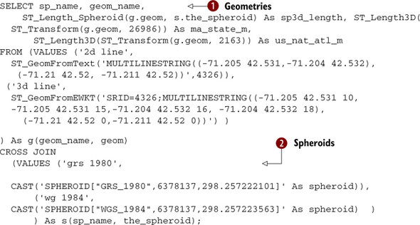
![]() In this example we compute the lengths of a 2D and a 3D multilinestring first by the spheroid function using both our spheroids.
Then we transform our lon lat coordinates to Massachusetts state plane projection and use the regular length 3D function.
We repeat the transform exercise but use the U.S. National Atlas projection.
In this example we compute the lengths of a 2D and a 3D multilinestring first by the spheroid function using both our spheroids.
Then we transform our lon lat coordinates to Massachusetts state plane projection and use the regular length 3D function.
We repeat the transform exercise but use the U.S. National Atlas projection. ![]() The spheroid object is another PostGIS object—the name is arbitrary, but the semi major axis (6378137 for both) and inverse
flattening (298...) are relevant. In terms of accuracy, the state plane is the most accurate followed by both spheroids. The
U.S. National Atlas is usually accurate within 10 meters (depending on length/distance), but it has the advantage that it
covers all of continental United States and can be used in all PostGIS planar operations.
The spheroid object is another PostGIS object—the name is arbitrary, but the semi major axis (6378137 for both) and inverse
flattening (298...) are relevant. In terms of accuracy, the state plane is the most accurate followed by both spheroids. The
U.S. National Atlas is usually accurate within 10 meters (depending on length/distance), but it has the advantage that it
covers all of continental United States and can be used in all PostGIS planar operations.
The output of the listing 4.5 is shown in table 4.6. Note that the spheroid (sp3d_ length) for 2D geometries is most similar to the Massachusetts state plane. For 3D geometries, the sp3d_length is a bit larger because it takes into consideration the Z coordinate.
Table 4.6. Results of query in listing 4.5
|
geom_name |
sp3d_length |
ma_state_m |
us_nat_atl_m |
|
|---|---|---|---|---|
| grs 1980 | 2d line | 220.337420025626 | 220.33319845914 | 220.759524564227 |
| wg 1984 | 2d line | 220.337387457848 | 220.33319845914 | 220.759524564227 |
| grs 1980 | 3d line | 227.341038849482 | 227.336817351126 | 227.763097850584 |
| wg 1984 | 3d line | 227.341006282557 | 227.336817351126 | 227.763097850584 |
They use the Z coordinate (elevation), assumed to be in meters.
They work only with linestrings and multilinestrings.
Units returned are always in meters.
Coordinates of the geometry are always assumed to be lon lat for PostGIS 1.5 and below.
Although there exists no ST_Perimeter_Spheroid function, it’s easy enough to simulate one by taking the ST_Boundary of a polygon and then the ST_Length_Spheroid of it. This works only for 2D polygons because ST_Boundary ignores the Z coordinate.
Next we’ll look at measurements with geography types in mind.
4.4.3. Measurement with geography type
All measurements based on geography type presume a geodetic model. In addition, all measurements return meters, but all coordinates are stored as WGS 84 lon lat degrees.
Aside from that, the measurement functions you’ll find for geography, for the most part, parallel those for geometry. ST_Length, ST_Area, ST_Distance, and ST_DWithin work as they do for geometry. The only difference is that these functions can take an optional argument named use_spheroid. If this is set to true or not passed in, then the calculations are done using a spheroid. If you pass in false, then all calculations are done using a sphere model. The sphere model is faster than the spheroid, but the difference is generally negligible. The measurements don’t consider the Z axis whatsoever. Unless you plan on journeying deep into the center of the earth or go on frequent jaunts into outer space, the curvature of the earth outrivals any consideration of height.
The ST_Perimeter function for geography is noticeably absent in PostGIS 1.5. To obtain the perimeter of a polygon geography type, you need to use ST_Length.
To demonstrate, in the following listing we’ll create the same types of objects we had for geometry data types except we’re using geography data types, and we’ll compare the spheroid against the sphere solutions.
Listing 4.6. Comparing spheroid and sphere calculations in geography
SELECT name, ST_Length(geog) As sp3d_lengthspheroid,
         ST_Length(geog, false) As sp3d_lengthsphere
FROM (VALUES ('2D Multilinestring',
        ST_GeogFromText('SRID=4326;
         MULTILINESTRING((-71.205 42.531, -71.204 42.532),
(-71.21 42.52, -71.211 42.52))')),
 ('3D Multilinestring',
          ST_GeogFromText('SRID=4326;
        MULTILINESTRING((-71.205 42.531 10, -71.205 42.531 15,
        -71.204 42.532 16,-71.204 42.532 18),
      (-71.21 42.52 0, -71.211 42.52 0))'))
) As foo (name, geog);
The results of the code run are shown in table 4.7.
Table 4.7. Results of the query in listing 4.6 demonstrating sphere versus spheroid lengths
|
geom_name |
length_spheroid |
length_sphere |
|---|---|---|
| 2d line | 220.337435990337 | 220.080539442185 |
| 3d line | 220.337435990337 | 220.080539442185 |
As you can see here, the Z coordinate is completely ignored for the geography ST_Length function. For this particular area the difference between the spheroid and sphere lengths is less than 1 meter.
Although the geography type has a fairly complete set of measurement functions, the other functions you’ll find available for the geometry type are for the most part missing for geography. The main exceptions to this rule are that geography does have an ST_Intersects, ST_Intersection, and ST_Buffer. It also has ST_Covers and ST_CoveredBy. The covers family of geography functions in PostGIS 1.5.1 and below support only polygon/point, point/polygon pairs.
4.5. Decomposition
You’ll find yourself often needing to extract parts of an existing geometry. You may need to find the closed linestring that encloses a polygon or the multipoint that constitutes a linestring. We call functions that extract and return one or more geometries decomposition functions.
4.5.1. Boxes and envelopes
Boxes are the unsung heroes of geometries. Though rarely useful to model terrestrial features, they play an important role in spatial queries. Often, when comparing the relative spatial orientation of two or more geometries, the question can be answered much faster for the bounding boxes of the geometries than for the geometries themselves. By encasing disparate and complicated geometries in bounding boxes, you only need to work with rectangles and can ignore the details of the geometries within. Borrowing from an engineering concept, bounding boxes are the black boxes of spatial analysis.
By definition, a box, or box2D, is the smallest two-dimensional box that fully encloses the geometry. (PostGIS also has another kind of box called box3D, but this is rarely used and doesn’t serve the same purpose as box2D.) All geometries have boxes, even points! Boxes aren’t geometries, but you can cast boxes into geometries. Naturally, casting a box to geometry will yield rectangular polygons, but you have to watch out for degenerate cases such as points, vertical lines, horizontal lines, or multipoints along a horizontal or vertical. The syntax for a 2D box is
BOX(p1,p2)
where p1 and p2 are points of any two opposite vertices.
PostGIS functions that create bounding boxes are ST_Box2D. The following listing shows some examples of these in action and the corresponding output.
Listing 4.7. ST_Box2D and casting a box to a geometry
SELECT name, ST_Box2D(geom) As box,
             ST_AsEWKT(CAST(geom As geometry)) As box_casted_as_geometry
FROM (
VALUES
('2D linestring', ST_GeomFromText('LINESTRING(1 2, 3 4)')),
('Vertical linestring', ST_GeomFromText('LINESTRING(1 2, 1 4)')),
('Point', ST_GeomFromText('POINT(1 2)')),
('Polygon', ST_GeomFromText('POLYGON((1 2, 3 4, 5 6, 1 2))')))
AS foo(name, geom);
The results of this query are shown in table 4.8. Vertical lines and single points produce degenerate boxes, and the geometry cast produces the same boxes as the geometry itself.
Table 4.8. Results of listing 4.7
|
name |
box |
box_casted_as_geometry |
|---|---|---|
| 2D linestring | BOX(1 2, 3 4) | POLYGON((1 2, 1 4, 3 4, 3 2, 1 2)) |
| Vertical linestring | BOX(1 2, 1 4) | LINESTRING(1 2, 1 4) |
| Point | BOX(1 2, 1 2) | POINT(1 2) |
| Polygon | BOX(1 2, 5 6) | POLYGON((1 2, 1 6, 5 6, 5 2, 1 2)) |
We mentioned that boxes aren’t geometries in their own right. If you need to obtain the geometry of the smallest rectangular box enclosing your geometry, use the ST_Envelope function to return the envelope. In cases where the underlying geometry has no width (such as a vertical linestring), no height (such as a horizontal linestring), or no width and no height (a point), ST_Envelope will simplify the geometry to either linestrings or points. In the following listing we revisit the previous example, but this time we include the ST_Envelope function.
Listing 4.8. Example of ST_Envelope
SELECT name, ST_Box2D(geom) AS box,
             ST_AsEWKT(ST_Envelope(geom)) AS env
FROM (
VALUES
('2D linestring', ST_GeomFromText('LINESTRING(1 2, 3 4)')),
('Vertical linestring', ST_GeomFromText('LINESTRING(1 2, 1 4)')),
('Point', ST_GeomFromText('POINT(1 2)')),
('Polygon', ST_GeomFromText('POLYGON((1 2, 3 4, 5 6, 1 2))'))
)
AS foo(name, geom);
Table 4.9 shows the output of the query. Observe that for degenerate cases such as a vertical linestring and point, the envelope is the same as the input geometry.
Table 4.9. Results of the code in listing 4.8
|
name |
box |
env |
|---|---|---|
| 2D linestring | BOX(1 2, 3 4) | POLYGON((1 2, 1 4, 3 4, 3 2, 1 2)) |
| Vertical linestring | BOX(1 2,1 4) | LINESTRING(1 2, 1 4) |
| Point | BOX(1 2, 1 2) | POINT(1 2) |
| Polygon | BOX(1 2, 5 6) | POLYGON((1 2, 1 6, 5 6, 5 2, 1 2)) |
Next we’ll look at coordinates.
4.5.2. Coordinates
ST_X and ST_Y are a pair of functions that you can use to return the underlying coordinates of points. They’re generally combined with ST_Centroid to get the X and Y coordinates of a centroid for non-point geometries.
The ST_Xm functions can be applied to all geometries and bounding boxes and are used to return the minimum/maximum X coordinate of each geometry.
The ST_Xm functions are defined only for box3D objects, but because there’s an autocast in place that converts a geometry to a box3D, you can use it directly on geometries. However, you can’t use it on the text representation of geometries, as demonstrated in our discussion on autocasts.
They’re rarely used alone but are in general combined with each other to arrive at the pseudo width, height, and so forth of a geometry. We’ll demonstrate their use when we talk about translation.
4.5.3. Boundaries
ST_Boundary works with all geometries and returns the geometry that determines the separation between the points in the geometry and the rest of the coordinate space. This particular way of defining boundary will make matters easy when we discuss interaction between two geometries in chapter 5. Also note that the boundary of a geometry is at least one dimension lower than the geometry itself. One common use of ST_Boundary is to break apart polygons and multipolygons into their constituent rings. ST_Boundary ignores M and Z coordinates and currently doesn’t work with geometry collections or curved geometries. The following listing shows some examples of ST_Boundary in action.
Listing 4.9. Examples of ST_Boundary
SELECT name, ST_AsText(ST_Boundary(geom)) As WKT
FROM (VALUES
('Simple linestring',
             ST_GeomFromText('LINESTRING(-14 21,0 0,35 26)')),
('Non-simple linestring',
            ST_GeomFromText('LINESTRING(2 0,0 0,1 1,1 -1)')),
('Closed linestring',
          ST_GeomFromText('LINESTRING(52 218, 139 82,
          262 207, 245 261, 207 267, 153 207,
          125 235, 90 270, 55 244, 51 219, 52 218)')),
('Polygon',
           ST_GeomFromText('POLYGON((52 218, 139 82, 262 207,
       245  261, 207 267, 153 207, 125 235, 90 270,
        55  244, 51 219, 52 218))')),
 ('Polygon with holes',
          ST_GeomFromText('POLYGON((-0.25 -1.25,-0.25 1.25,2.5 1.25,
        2.5 -1.25,-0.25 -1.25),(2.25 0,1.25 1,1.25 -1,2.25 0),
         (1 -1,1 1,0 0,1 -1))'))
)
AS foo(name, geom);
The output of listing 4.9 is shown in table 4.10 and figure 4.1.
Table 4.10. Output of listing 4.9
|
name |
WKT |
|---|---|
| Simple linestring | MULTIPOINT(-14 21,35 26) |
| Non-simple linestring | MULTIPOINT(2 0,1 -1) |
| Closed linestring | MULTIPOINT EMPTY |
| Polygon | LINESTRING(52 218,139 82,262 207,245 261,207 267,153 207,125 235, 90 270,55 244,51 219,52 218) |
| Polygon with holes | MULTILINESTRING((-0.25 -1.25,-0.25 1.25,2.5 1.25,2.5 -1.2 5,-0.25 -1.25), (2.25 0,1.25 1,1.25 -1,2.25 0),(1 -1,1 1,0 0,1 -1)) |
Figure 4.1. Simple linestring, polygon, and polygon with holes overlaid with their boundaries from the code in listing 4.9

Looking at the query and its output, you can surmise the following behavior of ST_Boundary:
- An open linestring, either simple or non-simple, will return a multipoint made up of exactly two points, one for each of the end points.
- A closed linestring has no boundary points.
- A polygon without holes will return a linestring of the exterior ring.
- A polygon with holes will return a multilinestring made up of closed linestrings for each of its rings. The first element of the multilinestring will always be the exterior ring.
- A multipolygon will always return a multilinestring
A more specialized cousin of ST_Boundary is ST_ExteriorRing. This function accepts only polygons and returns the exterior ring. If you’re trying to find the outer boundary of a polygon, ST_ExteriorRing will perform faster than ST_Boundary, but as its name suggests it won’t return the inner rings. You can use ST_InteriorRingN to grab individual interior rings.
4.5.4. Point marker for a geometry: centroid, point on surface, and nth point
We’ve all seen maps where small geometries are reduced to a single point to unclutter the visual representation. Most maps use a star to indicate capital cities rather than the city boundaries. Should you zoom in enough on any online map, for example, to the street level, you may find a labeled dot where you expect to see a huge polygon. Try this on a top-secret military installation. You zoom in enough and you won’t see any of the details you expect but just a dot telling you that it’s a place the government doesn’t want you to ever visit.
In PostGIS, ST_Centroid and to a lesser extent ST_PointOnSurface are often used to provide a point marker for polygons. You should think of the centroid of a geometry as the center of gravity as if every point in the geometry had equal mass. The only caveat is that the centroid may not lie within the geometry itself; think donuts or bagels. The ST_Centroid function works for all valid two-dimensional geometries including geometry collections but not curved geometries. For 3D geometries, it ignores the Z coordinate.
ST_Centroid sometimes produces undesirable visual results when the point isn’t on the geometry itself. Take the island nation of FSM (Federated States of Micronesia); its ST_Centroid is most likely somewhere in the Pacific Ocean. If you provide a mapping service, you probably don’t want people sailing to FSM and failing to end up on dry land. For this situation ST_PointOnSurface comes to the rescue. It always returns the same point for a given geometry. ST_PointOnSurface works for all geometries except curved geometries. For points, linestrings, multipoints, and multilinestrings it does consider the M and Z coordinates and returns a point that’s usually one used to define the geometry. For polygons, it cuts out the M and Z coordinates.
In the following listing, we compare the output of ST_Centroid with that of ST_PointOnSurface for various geometries.
Listing 4.10. Centroid of various geometries
SELECT name, ST_AsEWKT(ST_Centroid(geom)) As centroid,
ST_AsEWKT(ST_PointOnSurface(geom)) As point_on_surface
FROM (VALUES ('Multipoint', ST_GeomFromEWKT('MULTIPOINT(-1 1, 0 0, 2 3)')),
('Multipoint 3D', ST_GeomFromEWKT('MULTIPOINT(-1 1 1, 0 0 2, 2 3 1)')),
('Multilinestring', ST_GeomFromEWKT('MULTILINESTRING((0 0,0 1,1 1),
(-1 1,-1 -1))')),
('Polygon',
ST_GeomFromEWKT('POLYGON((-0.25 -1.25,-0.25 1.25,2.5 1.25, 2.5 -1.25,-0.25
-1.25), (2.25 0,1.25 1,1.25 -1,2.25 0), (1 -1,1 1,0 0,1 -1))')))
As foo(name, geom);
The code in listing 4.10 outputs both the centroid and the point on the surface of various geometries. Although the centroid may not always be part of the geometry, the point on the surface is.
Figure 4.2 shows the centroid overlaid with the original geometry that’s listed in table 4.11.
Figure 4.2. Geometries and centroids (denoted by stars) generated from the code in listing 4.10. Observe that the centroid isn’t always a point on the geometry.

Table 4.11. Output of query in listing 4.10
|
name |
centroid |
point_on_surface |
|---|---|---|
| Multipoint | POINT(0.333333333333333 1.33333333333333) |
POINT(-1 1) |
| Multipoint 3D | POINT(0.333333333333333 1.33333333333333) |
POINT(-1 1 1) |
| Multilinestring | POINT(-0.375 0.375) | POINT(0 1) |
| Polygon | POINT(1.125 0) | POINT(-0.125 0) |
Figure 4.3 shows the original geometries in listing 4.10 with the point on the surface overlaid, as listed in table 4.11.
Figure 4.3. Geometries and stars representing the point on the surface generated from code in listing 4.10

ST_Centroid and ST_PointOnSurface are both OGC/MM spatial functions, but the specification applied these functions only to surfaces geometries, such as polygons and multipolygons. They can be conveniently extended to other geometry types as many databases do, but you have to watch for differences when porting between different databases. PostGIS extends these two functions to work with other geometries. IBM DB II extends ST_Centroid to apply to other geometries but not ST_PointOn-Surface. SQL Server 2008 does the opposite and supports ST_Centroid for surface geometries only and ST_PointOnSurface for all geometries. Oracle Spatial supports them only for surface geometries.
A convenient little function that works only with linestrings and circularstrings is ST_PointN. It returns the nth point on the linestring, with indexing starting at 1. Here’s a quick example:
SELECT ST_AsText(
   ST_PointN(
     ST_GeomFromText('LINESTRING(1 2, 3 4, 5 8)'),
    2)
);
This returns
POINT(3 4)
Helpful, isn’t it?
4.5.5. Breaking down multi and collection geometries
Both ST_GeometryN and ST_Dump are useful for exploding multi and collection geometries into their component geometries. ST_Dump and ST_GeometryN don’t quite return the same answer, with the main difference being that ST_Dump recursively dumps all geometries in multi and collection, whereas ST_GeometryN goes down only a single level.
Strictly speaking, ST_Dump returns not a geometry but rows of geometry_dump objects. The geometry_dump object is a custom type installed with PostGIS and has two members. The first member of the dump object is the path. This member is a one-dimensional array indicating the depth at which the extracted geometry was found. The numbering scheme is intuitive. For example, if you have a geometry collection of multipolygons, {3, 2} would mean the third element of the collection, second polygon in the multipolygon. The second member of the geometry_dump is the geom property. This contains the exploded geometry for that given path. The path is useful if you ever need to reconstitute the original geometry. The other benefit of ST_Dump is that as of 1.3.6, ST_Dump can be used to explode curved geometries such as COMPOUNDCURVES, whereas ST_GeometryN can only explode multicurves, curved geometries, and other standard multi types.
PostGIS 1.5 introduced a new function called ST_DumpPoints, which works much like ST_Dump except it recursively dumps out all the points of a geometry collection or non-collection geometry. We have a demonstration of this in chapter 10 of our R example and use it to form a spatial dataframe in R.
Following is a demonstration of ST_Dump:
SELECT gid, (ST_Dump(geom)).path As exploded_path,
     ST_AsEWKT((ST_Dump(geom)).geom) As exploded_geometry
FROM (VALUES (1,
   ST_GeomFromEWKT('MULTIPOLYGONM(((2.25 0 3,1.25 1 2,
     1.25 -1 3,2.25 0 1)),
        ((1 -1 1,1 1 2,0 0 1,1 -1 1)))')),
 (2, ST_GeomFromEWKT('GEOMETRYCOLLECTION(
   MULTIPOLYGON(((2.25 0,1.25 1,1.25 -1,2.25 0)),
     ((1 -1,1 1,0 0,1 -1)) ),
   MULTIPOINT(1 2, 3 4), LINESTRING(5 6, 7 8),
     MULTICURVE(CIRCULARSTRING(1 2, 0 4, 2 8), (1 2, 5 6)))'))
) As foo(gid, geom);
You can see the results in table 4.12.
Table 4.12. Results of the previous code
|
gid |
exploded_path |
exploded_geometry |
|---|---|---|
| 1 | {1} | POLYGONM((2.25 0 3, 1.25 1 2, 1.25 -1 3, 2.25 0 1)) |
| 1 | {2} | POLYGONM((1 -1 1, 1 1 2, 0 0 1, 1 -1 1)) |
| 2 | {1, 1} | POLYGON((2.25 0,1.25 1,1.25 -1,2.25 0)) |
| 2 | {1, 2} | POLYGON((1 -1,1 1,0 0,1 -1)) |
| 2 | {2, 1} | POINT(1 2) |
| 2 | {2, 2} | POINT(3 4) |
| 2 | {3} | LINESTRING(5 6, 7 8) |
| 2 | {4, 1} | CIRCULARSTRING(1 2, 0 4, 2 8) |
| 2 | {4, 2} | LINESTRING(1 2, 5 6) |
ST_GeometryN extracts the nth geometry in a multi or collection geometry. It returns the single extracted geometry, doesn’t recurse, and doesn’t report the depth. Use ST_GeometryN when you have just one geometry to extract. If you find yourself needing to repeatedly call ST_GeometryN to explode all constituent geometries, you should use ST_Dump; otherwise you’ll suffer severe performance penalties. The following listing demonstrates use of ST_GeometryN. We use the PostgreSQL generate_ series function combined with the ST_NumGeometries function to extract all the geometries found in the first level of depth. The results are shown in table 4.13.
Table 4.13. Results of code in listing 4.11
|
gid |
extracted_geometry |
|---|---|
| 1 | POLYGONM((2.25 0 3, 1.25 1 2, 1.25 -1 3, 2.25 0 1)) |
| 1 | POLYGONM((1 -1 1, 1 1 2, 0 0 1, 1 -1 1)) |
| 2 | MULTIPOLYGON(((2.25 0, 1.25 1, 1.25 -1, 2.25 0)), ((1 -1, 1 1, 0 0, 1 -1))) |
| 2 | MULTIPOINT(1 2, 3 4) |
| 2 | LINESTRING(5 6, 7 8) |
| 2 | MULTICURVE(CIRCULARSTRING(1 2, 0 4, 2 8), (1 2, 5 6)) |
Listing 4.11. Example using ST_GeometryN with generate_series
SELECT gid, ST_AsEWKT(ST_GeometryN(geom,
     generate_series(1,ST_NumGeometries(geom)))) As extracted_geometry
FROM (VALUES (1,
        ST_GeomFromEWKT('MULTIPOLYGONM(((2.25 0 3, 1.25 1 2,
          1.25 -1 3, 2.25 0 1)),
        ((1 -1 1, 1 1 2, 0 0 1, 1 -1 1)))')),
(2, ST_GeomFromEWKT('GEOMETRYCOLLECTION(
       MULTIPOLYGON(((2.25 0, 1.25 1, 1.25 -1, 2.25 0)),
 ((1 -1, 1 1, 0 0, 1 -1))),
    MULTIPOINT(1 2, 3 4), LINESTRING(5 6, 7 8),
       MULTICURVE(CIRCULARSTRING(1 2, 0 4, 2 8), (1 2, 5 6)))'))
) As foo(gid, geom);
ST_DumpRings is less used than ST_Dump but is invaluable for breaking up multiringed polygons into smaller polygons. Unlike the ST_ExteriorRing and ST_InteriorRingN functions, which return the exterior ring and nth ring of a polygon as linestrings, ST_DumpRings converts them to single-ringed polygons. ST_DumpRings is tremendously useful for polygons with lots of holes, especially if you need all the rings. The alternative is to dump each ring using ST_InteriorRingN and then use ST_BuildArea to form the polygon.
Because the output of the function could contain multiple rows, ST_DumpRings returns geometry_dump objects. Because a valid polygon can only have one exterior ring, the path array uses zero to denote the exterior ring and then starts numbering at one. In our example that follows, we use ST_DumpRings to extract the exterior ring and the first ring, followed by an example of ST_ExteriorRing and ST_InteriorRingN to do the same. The results are shown in table 4.14.
Table 4.14. Results of query in previous code
|
exterior_ring_polygon |
interior_ring1_polygon |
|---|---|
| POLYGON((-0.25 -1.25, -0.25 1.25, 2.5 1.25...)) | POLYGON((2.25 0, 1.25 1, 1.25 -1, 2.25 0)) |
SELECT MAX(CASE WHEN path[1] = 0
    THEN ST_AsText(geom) ELSE NULL END) As exterior_ring_polygon,
    MAX(CASE WHEN path[1] = 1 THEN ST_AsText(geom)
       ELSE NULL END) As interior_ring1_polygon
FROM ST_DumpRings(
     ST_GeomFromText('POLYGON((-0.25 -1.25, -0.25 1.25,
   2.5 1.25, 2.5 -1.25, -0.25 -1.25),
  (2.25 0, 1.25 1, 1.25 -1, 2.25 0),
  (1 -1, 1 1, 0 0, 1 -1))')) WHERE path[1] IN(0,1);
We now perform the same extraction using ST_ExteriorRing and ST_InteriorRingN. Remember that these two functions return the rings as linestrings. The results are shown in table 4.15.
Table 4.15. Result of query in previous code
|
exterior_ring |
interior_ring1 |
|---|---|
| LINESTRING(-0.25 -1.25, -0.25 1.25, 2.5 1.25...) | LINESTRING(2.25 0, 1.25 1, 1.25 -1, 2.25 0) |
SELECT ST_AsText(ST_ExteriorRing(geom)) As exterior_ring,
ST_AsText(ST_InteriorRingN(geom,1)) As interior_ring1
FROM ST_GeomFromText('POLYGON((-0.25 -1.25,-0.25 1.25,2.5 1.25,
2.5 -1.25,-0.25 -1.25), (2.25 0,1.25 1,1.25 -1,2.25 0),
(1 -1,1 1,0 0,1 -1))') As geom;
Now that you know how to take geometries apart, you need to know how to put geometries together. We’ll move on to composition functions in the next section.
4.6. Composition
We already covered how to create geometries from non-geometry data, either text or binary. In this section, we’ll show you how to put together geometries from other geometries.
4.6.1. Making points
Points are the most elementary geometries. Points can be created from X-Y coordinates with two functions: ST_Point and ST_MakePoint. Coordinates aren’t geometries, but we feel they’re more related to geometries than text representations. Hence, we classify ST_Point and ST_MakePoint as composition functions.
ST_Point works only for 2D coordinates but is found in most spatial databases. ST_MakePoint and a variant, ST_MakePointM, can accept 2DM, 3D, and 4D coordinates in addition to 2D, but these two functions are PostGIS-specific. Syntax is the same for all three. The first argument is the coordinates separated by commas. Because these functions don’t take SRID as an argument, you need to combine them with ST_SetSRID to denote a spatial reference system.
You may ask yourself what these two additional functions offer beyond the common ST_GeomFromText besides a different import format. To put it concisely: speed and precision. Creating a handful or even a few hundred points doesn’t take much time, but loading files with millions of point data with many significant digits (a common task when working with data collected via instrumentation) is a different matter, and you’ll certainly come to prefer ST_Point or ST_MakePoint over ST_GeomFromText. To illustrate these two functions, in listing 4.12 we’ll simulate reading data points from tracking devices attached to gray whales as they make their annual migration from Baja California to the Bering Sea. Depending on the interval of reads and the number of whales we track, the number of data points coming into our database can be quite overwhelming, making speed an important consideration for import.
Listing 4.12. Point constructor functions

This code demonstrates various overloads to the ST_Point and ST_MakePoint functions. In ![]() , we employ an extra unit M to store time as a serial. For example, if we take readings every 5 hours, then M=1 would mean
this reading was taken 5 hours from the start time, M=2, 10 hours, and so on. If you’re keeping data as individual points,
this isn’t terribly useful, but if you later decide to stitch them together into a LINESTRINGM, then the time slots are encoded
in the line and there’s only one record for each whale instead of a separate array for the timings.
, we employ an extra unit M to store time as a serial. For example, if we take readings every 5 hours, then M=1 would mean
this reading was taken 5 hours from the start time, M=2, 10 hours, and so on. If you’re keeping data as individual points,
this isn’t terribly useful, but if you later decide to stitch them together into a LINESTRINGM, then the time slots are encoded
in the line and there’s only one record for each whale instead of a separate array for the timings. ![]() We may be interested in knowing how far Mr. Whale dove before coming to surface for air, so we use the Z coordinate to store
the depth. SRID 4326 is unprojected data, and ST_Transform currently returns the Z coordinate unchanged.
We may be interested in knowing how far Mr. Whale dove before coming to surface for air, so we use the Z coordinate to store
the depth. SRID 4326 is unprojected data, and ST_Transform currently returns the Z coordinate unchanged. ![]() We include both Z and M. M is an additional measurement that you can use to store anything and can mean time or distance
from the starting point.
We include both Z and M. M is an additional measurement that you can use to store anything and can mean time or distance
from the starting point.
The output of listing 4.12 is shown in table 4.16. Note that all except for the whale with M use POINT but have varying number of coordinates.
Table 4.16. Output from query in listing 4.12
|
whale |
spot |
|---|---|
| Mr. Whale | SRID=4326; POINT(-100.499 28.7015) |
| Mr. Whale with M as time | SRID=4326; POINTM(-100.499 28.7015 5) |
| Mr. Whale with Z as depth | SRID=4326; POINT(-100.499 28.7015 0.5) |
| Mr. Whale with M and Z | SRID=4326; POINT(-100.499 28.7015 0.5 5) |
Next, we’ll make polygons.
4.6.2. Making polygons
ST_MakePolygon, ST_BuildArea, and ST_Polygonize all build polygons.
St_Makepolygon
ST_MakePolygon builds a polygon from a closed linestring representing the exterior ring. Optionally, it can accept as a second argument an array of closed linestrings for interior rings. ST_MakePolygon doesn’t validate the input linestrings in any way. This means that if you aren’t careful, and you pass in open linestrings or linestrings that can’t form polygons, you could end up with an error or fairly goofy polygon, such as polygons with holes outside the exterior ring or interior rings not completely contained by the exterior ring. The complete absence of validation does provide an advantage in speed. ST_MakePolygon runs much quicker than other functions for creating polygons and is the only one that won’t ignore Z and M coordinates. ST_MakePolygon accepts only closed linestrings as input—no multilinestrings, no collections of linestrings.
St_Buildarea
You can think of ST_BuildArea as the neater roommate of ST_MakePolygon. Unlike its more reckless counterpart, you can toss it whatever you like and it will organize what you’ve offered into valid polygons.
ST_BuildArea will accept linestrings, multilinestrings, polygons, multipolygons, and geometrycollections. You don’t have to worry about the order or the validity of the geometries that you feed into ST_BuildArea. It will check the validity of each input geometry, determine which geometries should be interior rings and which one should be the exterior ring, and finally reshuffle them to output polygons or multipolygons. ST_BuildArea won’t work with arrays. But this shortcoming is mitigated by the fact that it will accept multilinestrings and geometrycollection geometries. If you intend to feed the function an assortment of linestrings and polygons, perform an ST_Collect first to gather all the loose pieces into a single geometry.
All this neatness comes at a price: You sacrifice performance. If you’ve already sanitized your input geometries using another procedure and speed is of utmost importance, use ST_MakePolygon. If your input geometry came from suspect sources and you just want to see what area comes out, the sanitizing feature of ST_BuildArea will be worth the wait.
St_Polygonize
ST_Polygonize is a database aggregate function. As a database aggregate, its use makes sense only against an existing table with geometry columns. This function takes rows of linestrings and returns a geometry collection consisting of the possible polygons you can form from such linestrings. It’s often used when trying to formulate polygons from edge linestrings and then passed to ST_Dump to dump out the individual polygons as separate rows.
We demonstrate the use of all three polygon-making functions in the next listing.
Listing 4.13. ST_Polygonize, ST_BuildArea, ST_MakePolygon

First we create the example table. ![]() ST_MakePolygon has two variants.
ST_MakePolygon has two variants. ![]() The simpler version takes an outer ring and forms a polygon without holes. In the second version
The simpler version takes an outer ring and forms a polygon without holes. In the second version ![]() , we’re using the ST_MakePolygon (outer ring, array of inner rings) to form a polygon with holes. We’re also using two SQL
constructs somewhat unique to PostgreSQL. The first is the generate_series function, which generates a number between start and end (for this trivial example it will generate
a set of numbers between 2 and 2 because there are only two linestrings in our multilinestring example and the first is reserved
for the exterior ring. We then use this to extract the second linestring. (If there were more linestrings or more multilinestrings,
then the generate series could be 2 to 3 or 2 to 4 and so on.) We then use the array[..] constructor in PostgreSQL, which
can take a list of elements, or an SQL statement to populate the array (in our case we’re using the SQL). ST_MakePolygon can
now accept our array of linestrings as the second argument and use it to form the interior rings of our polygon. The output
is shown in table 4.17.
, we’re using the ST_MakePolygon (outer ring, array of inner rings) to form a polygon with holes. We’re also using two SQL
constructs somewhat unique to PostgreSQL. The first is the generate_series function, which generates a number between start and end (for this trivial example it will generate
a set of numbers between 2 and 2 because there are only two linestrings in our multilinestring example and the first is reserved
for the exterior ring. We then use this to extract the second linestring. (If there were more linestrings or more multilinestrings,
then the generate series could be 2 to 3 or 2 to 4 and so on.) We then use the array[..] constructor in PostgreSQL, which
can take a list of elements, or an SQL statement to populate the array (in our case we’re using the SQL). ST_MakePolygon can
now accept our array of linestrings as the second argument and use it to form the interior rings of our polygon. The output
is shown in table 4.17.
Table 4.17. Results of query in listing 4.13
|
Function |
Polygon |
|---|---|
| ST_MakePolygon (1) | POLYGON((1 2, 3 4, 4 4, 1 2)) |
| ST_MakePolygon (2) | POLYGON((0 0, 4 4, 4 0, 0 0),(2 1, 3 1, 3 2, 2 1)) |
| ST_BuildArea | POLYGON((1 2, 3 4, 4 4, 1 2)) |
| ST_BuildArea | POLYGON((0 0, 4 4, 4 0, 0 0),(2 1, 3 1, 3 2, 2 1)) |
| ST_Polygonize | GEOMETRYCOLLECTION(POLYGON((1 2, 3 4, 4 4, 1 2)), POLYGON((0 0, 4 4, 4 0, 0 0), (2 1, 3 1, 3 2, 2 1)), POLYGON((2 1, 3 2, 3 1, 2 1))) |
In listing 4.13, ST_MakePolygon and ST_BuildArea return the same answers when a linestring and multilinestrings form well-formed geometries; however, for ST_MakePolygon we had to break our selects to separate the linestrings from multilinestrings. ST_Polygonize is an aggregate function; it takes rows of geometries and returns one geometry collection. It’s incapable of creating polygons with holes, so every ring in the multilinestring becomes a polygon in its own right.
4.6.3. Promoting single to multi geometries
The ST_Multi function is used quite often in PostGIS, mostly to promote points, linestrings, and polygons to their multi counterparts even if they have only a single geometry. If a geometry is already a multi variety, then it remains unchanged. Its main use case is to ensure that all geometries in a table column are of the same geometry type for consistency. For instance, suppose you obtained polygons for all nations. The Kingdom of Lesotho could come in as a single polygon because it’s a tiny, landlocked enclave, whereas Indonesia will come in as a multipolygon. To keep your column consistent, you’d promote Lesotho to a multipolygon.
In the next section, we’ll cover how to simplify our geometries.
4.7. Simplification
For this section we’ll cover the three functions ST_SnapToGrid, ST_Simplify, and ST_SimplifyPreserveTopology. These functions behave quite differently from one another, but they all try to achieve the same goal: reducing the bytes necessary to describe a geometry. Simplification functions become important when passing geometries across the internet. Despite recent advances, bandwidth is still a precious commodity, especially with wireless devices. With a tiny, black and white, 200 x 300 resolution GPS screen, transmitting geometries with thousands of vertices or coordinates with a monstrous number of significant digits is certainly overkill.
4.7.1. Coordinate rounding using ST_SnapToGrid
ST_SnapToGrid reduces the weight of a geometry by rounding the coordinates. If after rounding, two or more adjacent coordinates become indistinguishable, it will automatically keep only one of them, thus reducing the number of vertices.
There are four variants of this function. The most common one takes one argument for tolerance and rounds the X and Y coordinates while leaving Z and M intact. ST_SnapToGrid doesn’t remove Z and M coordinates. Other variants can round all four coordinates or allow you to specify offsets to indicate where the grid starts.
One common use of ST_SnapToGrid is to trim those extra floating-point decimals introduced by ST_Transform. Those extra digits can degrade performance and are generally a nuisance if the precision isn’t needed. Another use of ST_SnapToGrid is to group distinct nearby points into a single representational point. For example, if you obtained point data for every school in the country but care only about the location of school districts, then collapsing all the schools down to a single point would be the way to go, especially with data on a national scale.
As with most simplifying operations, you should exercise restraint. Too ambitious rounding can inadvertently turn a valid polygon into an invalid one.
SELECT pow(10, -1*n)*5 As tolerance,
ST_AsEWKT(ST_SnapToGrid(
  ST_GeomFromEWKT('SRID=4326;
  LINESTRING(-73.81309 41.74874, -73.81276 41.74893,
   -73.812765 41.74895, -73.81307 41.74896)'),
   pow(10, -1*n)*5)) As simplified_geometry
FROM generate_series(3,6) As n
ORDER BY tolerance;
You can see the results in table 4.18.
Table 4.18. Results of the query in the previous code
|
tolerance |
simplified_geometry |
|---|---|
| 0.000005 | SRID=4326; LINESTRING(-73.81309 41.74874, -73.81276 41.74893, -73.812765 41.74895, -73.81307 41.74896) |
| 0.00005 | SRID=4326; LINESTRING(-73.8131 41.74875, -73.81275 41.74895, -73.81305 41.74895) |
| 0.0005 | SRID=4326; LINESTRING(-73.813 41.7485, -73.813 41.749) |
| 0.005 | NULL |
In this example we generate a number between 3 and 6 and then use that to round the coordinates of our linestring. Notice that when we reach rounding tolerance of 0.005, our linestring disappears. This is because ST_SnapToGrid will always return the same output geometry type as the input, but if you round to .005, the input geometry has collapsed into a single point and is no longer a linestring.
4.7.2. Simplifying geometries
ST_Simplify and ST_SimplifyPreserveTopology both reduce the weight of a geometry by reducing the number of vertices of the geometry, using some variant of the Douglas-Peucker algorithm. The ST_SimplifyPreserveTopology function is newer than ST_ Simplify and has safeguards against oversimplification. In extreme cases of oversimplification, the geometry could very well vanish, as shown previously, or become invalid. ST_SimplifyPreserveTopology is generally preferred over the older ST_Simplify even though it’s a bit slower.
Both ST_Simplify and ST_SimplifyPreserveTopology take a second argument, which we’ll term tolerance. This can be roughly treated as the unit of length between the vertices at which you’d want to collapse the vertices into one. For example, if you set the argument to 100, the two functions will try to collapse any vertices spaced 100 units apart. As you increase the tolerance, you’ll experience more simplification. Putting it another way, the more tolerant you are of losing vertices, the more simplification you can achieve.
These two simplifying functions, unlike ST_SnapToGrid, don’t preserve M and Z coordinates and will even remove them if present. They also work only for linestrings, multilinestrings, polygons, multipolygons, and geometry collections containing these geometries. For multipoints they return the same input geometry without any simplification. The reason for this is that ST_Simplify and ST_SimplifyPreserveTopology require edges (lines between vertices) to achieve simplification. Multipoints don’t have edges.
ST_Simplify and ST_SimplifyPreserveTopology assume planar coordinates. Should you use these functions with lon lat data (SRID 4326), the resultant geometry can range from slightly askew to completely goofy. First transform your lon lat to a planar coordinate, apply ST_Simplify, and then transform back to lon lat.
The following code compares the two functions:
SELECT pow(2, n) as tolerance,
  ST_AsText(ST_Simplify(geom, pow(2, n))) As ST_Simplify,
  ST_AsText(
    ST_SimplifyPreserveTopology(geom, pow(2, n)))
    As ST_SimplifyPreserveTopology
FROM (SELECT
  ST_GeomFromText('POLYGON((10 0, 20 0, 30 10, 30 20,
  20 30, 10 30, 0 20, 0 10, 10 0))') As geom
) As foo CROSS JOIN generate_series(2,4) As n;
Table 4.19 shows the results of our comparison.
Table 4.19. Results of query in previous code (split into two sections for readability)
|
tolerance |
ST_Simplify |
|---|---|
| 4 | POLYGON((10 0, 20 0, 30 10, 30 20, 20 30, 10 30, 0 20, 0 10, 10 0)) |
| 8 | POLYGON((10 0, 30 10, 20 30, 0 20, 10 0)) |
| 16 | NULL |
| tolerance | ST_SimplifyPreserveTopology |
| 4 | POLYGON((10 0, 20 0, 30 10, 30 20, 20 30, 10 30, 0 20, 0 10, 10 0)) |
| 8 | POLYGON((10 0, 30 10, 20 30, 0 20, 10 0)) |
| 16 | POLYGON((10 0, 30 10, 20 30, 0 20, 10 0)) |
Notice that once you reach a tolerance of 16 with ST_Simplify, the geometry vanishes. But ST_SimplifyPreserveTopology reduces the eight-sided polygon to a four-sided polygon and stops there regardless of the tolerance. Figure 4.4 demonstrates the difference between ST_Simplify and ST_SimplifyPreserveToplogy for the eight-sided version.
Figure 4.4. ST_Simplify and ST_SimplifyPreserveTopology, going from an eight-sided polygon to a four-sided polygon

This simplification stops there, regardless of how high you raise the tolerance.
4.8. Summary
In this chapter we’ve started to cover the most commonly used functions in PostGIS. For the moment we concentrated on functions with a single geometry as argument. We developed a loose classification scheme to organize the myriad of unary functions in PostGIS. Starting with constructors, we then moved on to getters and setters, followed by decomposition and composition functions. We ended the chapter with simplification functions. These popular functions constitute but a small subset of all the unary functions available in PostGIS. We highly recommend you to peruse the official PostGIS documentation to see all that are available. You may find the number of functions overwhelming at first, but on closer examination, you’ll find that many functions are closely related and fit nicely into our taxonomy. We also advise you to refer to the documentation before using any of the functions we described.
In the next chapter we’ll continue our exploration of PostGIS functions by covering functions that take two or more geometries as input: binary functions. You’ll find binary functions to be far more useful, and perhaps more interesting, for answering questions regarding your data, but don’t disdain the unaries. Geometries for binary functions almost always have to be prepared by some type of unary function.