20

Sliding Electrical Contacts (Graphitic Type Lubrication)

Kiochiro Sawa and Erle I. Shobert II

Let the world slide, let the world go

Be Merry Friends, John Heywood

CONTENTS

20.1    Introduction

20.2    Mechanical Aspects

20.2.1    Hardness

20.2.2    Friction and Wear

20.2.3    Tunnel Resistance and Vibration

20.3    Chemical Aspects

20.3.1    Oxidation

20.3.2    Moisture Film

20.4    Electrical Effects

20.4.1    Constriction Resistance

20.4.2    Film Resistance

20.4.3    Fundamental Aspects of Commutation

20.4.4    Equivalent Commutation Circuit and DC Motor Driving Automotive Fuel Pump

20.4.5    Arc Duration and Residual Current

20.5    Thermal Effects

20.5.1    Steady State

20.5.2    Actual Temperature

20.5.3    Thermal Mound

20.6    Brush Wear

20.6.1    Holm’s Wear Equation

20.6.2    Flashes and Smutting

20.6.3    Polarities and Other Aspects

20.7    Brush Materials and Abrasion

20.7.1    Electro- and Natural Graphite Brushes

20.7.2    Metal Graphite Brush and Others

20.8    Summary

References

20.1  Introduction

Sliding contacts are widely used to transfer electric power and/or signals between stationary devices and moving devices. Although these contacts move relative to each other, much of what has been discussed previously in this book on stationary contacts also applies to sliding contacts albeit with some modifications.

As shown in Figure 20.1, real contact area is much smaller than apparent contact area [1]. And conductive area is smaller than real contact area. Therefore, like stationary contacts a constriction resistance is one of the important factors in the contact resistance. But the conducting surfaces on sliding contacts are usually long narrow strips [2].

The oxidation of metal surfaces, discussed previously in Chapter 2, applies in principle to sliding contacts. The fritting or breakdown of insulating surface films, considered in Chapter 1, takes place in sliding contacts. The disturbance owing to arcing in Chapter 9 takes place on the edges of commutator bars and brushes and contributes to brush and commutator wear. Surface films owing to condensed organic materials, discussed in Chapter 7, are involved in certain sliding contact applications.

The calculation of the temperature rise owing to the electrical currents discussed in Chapter 1 can be adapted to sliding contacts with the modification for the fact that one side of the contact is moving [2]. Depending on the mechanical design, the conducting surfaces may move around on both the moving and stationary contacts. With special designs, the contact surfaces may be stabilized for short periods on the stationary contact surface. Thus, we see that there is a considerable amount of the theory of stationary contacts that applies to sliding contacts.

There are several aspects in which stationary and sliding contacts are fundamentally different. For example, with some exceptions for small contact forces on metal wires, any two clean metallic surfaces in vacuum will cold weld and seize so that the surfaces are destroyed during sliding (see Figure 20.2). This is true even for electrographite against electrographite. When the two surfaces approach each other to within atomic distances, the electron clouds of the two materials comingle and the surfaces act as though they were welded together. When this occurs in practice, the brushes disappear in a cloud of dust and are worn out in minutes (see Section 20.3).

Thus, the surfaces must be several atomic distances apart and conduction takes place across an insulating film, water in most applications, approximately two molecular layers thick by means of the tunnel effect. As discussed in Chapter 1, the tunnel effect permits electronic conduction through this film as described by quantum theory. As will be pointed out in Section 20.3, Holm has discussed the thickness of these moisture films (see Section 20.3). The resistance of these films increases steeply with film thickness so that an increase of an additional layer or two of the film would cause a drastic increase in the voltage of the contact.

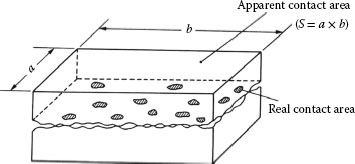
FIGURE 20.1
Apparent and real contact.

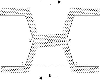
FIGURE 20.2
Rupture of a single contact.

It is fortunate that water provides the material film for most brush applications at sea level. It is effective at dew points above about −10°C and is usually not harmful until liquid water becomes present and affects insulation. For electrographite brushes against copper, two molecular layers or water give a tunnel effect voltage, ΔV, of about 0.2–0.3 V. Three molecular layers of water add an additional 1 V drop. Since the normal total voltage drop on electrographite brushes is about 1 V, it is readily seen that the two surfaces must slide consistently within 5–10 Å (0.5–1 nm) of each other. Other filming agents can replace water when it is not available.

Another basic difference between stationary and sliding contacts is friction. Friction has two effects. First is the heat generated by sliding that adds to the heat generated electrically in determining the temperature. At high speeds this can be appreciable, and while it is generated over the mechanical contact surface, which is usually larger than the electrical conducting surface, it still must be dissipated in the brush collector system. The second friction effect is concerned with friction-excited vibration (see Section 20.2). Many ordinary machines have the possibility of having certain natural periods excited by friction, but it is possible to eliminate this by proper design.

Another important factor, which is not always recognized, is the fact that for long-term operation, the electrical situation must be the same on each commutation bar or there must not be synchronous effects of variable currents on rings. Since the collector films are influenced by the current, the friction will vary where the current varies. If this takes place consistently on any section of the collector, vibrations and eventual burning will take place, with disastrous results. This is discussed in Section 20.4.

Finally, there is a fundamental difference in the philosophy for successful brush operation compared with stationary contacts. Since the film is such an important component, and since it is complicated by moisture, oxides, organic compounds in the atmosphere, and brush materials, it is necessary to have materials that have a certain controlled amount of abrasive action. This prevents overfilming and provides consistent operation over a wide variety of circumstances (see Section 20.7). In practical applications, this is achieved with metal and graphite materials, with the addition of known abrasives, and with abrasive forms of carbon and graphite.

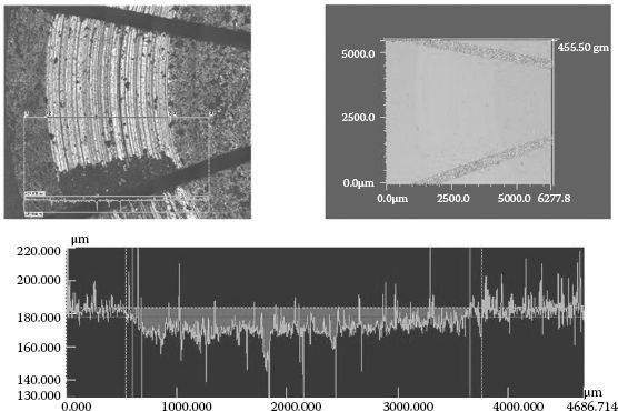
FIGURE 20.3
An example of laser microscopy analysis.

Recently, Finite Element Analysis and other simulation methods are used to examine phenomena of sliding contacts from electric, thermal and mechanical aspects [3]. In addition, the laser microscope and other analytical methods are used to evaluate friction wear and other parameters (see Figure 20.3) [4]. From fundamental viewpoints, the real area of contact between brush and copper ring has been measured, and the current density distribution was directly observed by using light emission diode wafer [5,6].

It should be noted that we are dealing in this section primarily with sliding contacts with graphite type lubrication. There are other types of sliding contacts, for example, fiber brushes and precious metal wires that operate on different fundamental bases: see Chapters 22 and 23. These are discussed in seperate sections below. With this background, we will discuss the mechanical, chemical, electrical, thermal, and material factors that work together in successful applications. Since we are dealing with phenomena, which are complicated combinations of mechanical, chemical and electrical effects, they are present at the same time, but they must be separated to understand the results and to solve the problems that arise.

20.2  Mechanical Aspects

There are reasons for considering the mechanical aspects of sliding electrical contacts first. The mechanical system determines several important factors which relate to operation, such as the radius of contact at the face of the brush, the possibility of friction-excited vibration, and the direction and characteristics of heat flow. Also, the mechanical system must ensure that the stationary and moving surfaces remain in contact at between 5 and 10 Å (0.5–1 nm) of each other owing to the reason mentioned later. This represents a distance of about two molecular layers of water.

20.2.1  Hardness

First, we consider the hardness.

Assuming that the deformation of two surfaces is elastic, the radius of their contact a is expressed by the following Hertz’s formula [1].

$a=\sqrt[3]{\frac{3}{4}P\left(\frac{1-{\text{μ}}_1^2}{E_1}+\frac{1-{\text{μ}}_2^2}{E_2}\right){\left(\frac{1}{r_1}+\frac{1}{r_2}\right)}^{-1}}$

(20.1)

where r₁, r₂: curvatures of two contacts, E₁, E₂: Young’s modulus of elasticity of two contacts, μ₁, μ₂: Poisson ratios of two contacts, and P: contact force.

When two contacts are sphere, centers of the spheres approach each other by y

$y=a^2\left(\frac{1}{r_1}+\frac{1}{r_2}\right)$

(20.2)

Actually, the surfaces have certain roughness and certain waviness. At contact make, asperities of one contact indent in the other contact. At small average pressure the indentations may be formed elastically. With increasing average pressure, indentations become plastically produced. Finally, almost all indentations could be deformed plastically, and the following equation is derived,

$P=H{A}_b$

(20.3)

where P: contact force, H: hardness, A_b: load bearing area.

However, actually, when some indentations deepen, other asperities obtain the opportunities to make contact. These initially generate shallow elastic indentations. So, the average pressure will be smaller than H, that is,

$\overline{p}=\text{ξ}H$

(20.4)

with ξ < 1. Hence,

$P=\text{ξ}H{A}_b$

(20.5)

Theoretically, the value of ξ is between 0 and 1, but according to measurements, the value is between 0.1 and 0.3 in many cases.

When two surfaces such as a ball and a plane are pressed together, the ball will indent into the plane until the elastic force supports the load. As the ball becomes larger for the same load, the surface pressure defined as the contact hardness becomes smaller as shown in Figure 20.4 [7]. Since we are dealing with relatively flat surfaces, the hardness that determines the surface area is the low point at specific depth 0. This is usually about two thirds of the value of the hardness at A′, B′, or C′ that represents a small ball on a plane. Values of the contact hardness are given for various brush materials in Table 20.1. Because of certain small eccentricities in the rotating collector, the radius of the brush face is always slightly larger than the radius of the collector. Thus, we have two cylinders in compression. In addition to the eccentricity which makes the brush radius r₂ larger than that of the collector r₂, there is usually some possible side play of the brush that makes the face saddle shaped. Thus, we have two spheres one inside the other and the formula for the radius of the contact is obtained from (Equation 20.1) with μ = 0.3 and E₁ = E₂ = E:

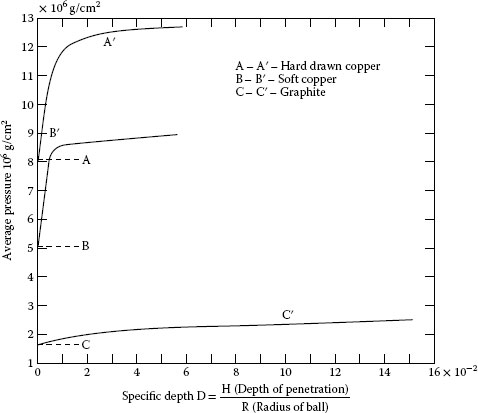
FIGURE 20.4
Contact hardness.

$a\prime =0.88\sqrt[3]{\frac{P}{E}{\left(\frac{1}{r_1}-\frac{1}{r_2}\right)}^{-1}}\left(\text{cm}\right)$

(20.6)

TABLE 20.1
Contact Hardness

Material	Contact Hardness
40 Cu 60 C	1.0 × 102 N mm−2
Resin-bonded graphite	2.6
Electrographite	2.9
Carbon graphite	3.5
Copper	4–9
Silver	3–7

where P is the force in grams and E is the elasticity of the softer brush materials. Going further, the elastic penetration, y, is given by

$y=\frac{a^{\prime 2}\left(r_2-r_1\right)}{r_1{r}_2}\left(\text{cm}\right)$

(20.7)

This elastic penetration is important since it provides the restoring force to permit the brush face to follow small variations on the collector surface such as low and high commutator bars. It is the only apparent mechanism that will permit the brush surface to follow known variations in collector surfaces.

The elastic recovery of the surface penetration should approach the speed of sound in the materials. This is faster than any commutator bar variation that is known in practice. Of course, the distance to be recovered must be within the limits of the penetration available at the brush face.

Thus, we have a means of providing that these surfaces stay within the 0.5–1.0 nm distance from each other that is required by the tunnel effect conduction.

20.2.2  Friction and Wear

The next mechanical effect is friction. The coefficient of friction is defined by the relation

$\text{μ}=\frac{F}{P}$

(20.8)

where F is the tangential friction force and P is the normal force. As Holm [8] pointed out,

$F=\text{ψ}{A}_b$

(20.9)

where Ψ is the shear strength of the film when normal sliding takes place and A_b is the load bearing area. Without a film Ψ becomes the shear strength of the weaker of the two contact materials.

In the elastically supported, plastically deformed surfaces A_b can be obtained from Equation 20.5,

$P=\text{ξ}H{A}_b$

(20.10)

Thus,

$\text{μ}=\frac{F}{P}=\frac{\text{ψ}}{\text{ξ}H}$

(20.11)

In this relation, Ψ is determined by the complex film consisting of the moisture film, the oxide film, and any other materials or contaminants that might be in the atmosphere. The adjuvant added to the brushes provides this film in vacuum. H is a material constant of the brush which is generally much softer than the collector, and ξ is a factor that can vary with the machine and its operating condition. For example, high brush friction as a result of light load running may be caused by a decrease in this factor as well as the decrease in temperature.

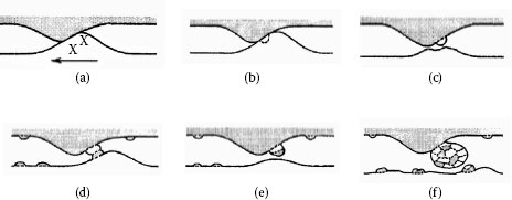
FIGURE 20.5
Transfer and growth wear model. (a) Contact; (b) Internal rupture; (c) Transfer element; (d) Attached transfer elements; (e) Transfer particle; (f) Grown transfer particle.

On the basis of the idea of adhesive wear, R. Holm proposed the following equation of wear,

$V=Z\frac{P\ell }{p_m}$

(20.12)

where V: wear volume, P: contact force, ?: sliding distance, p_m: hardness of softer contact and Z: a constant called wear factor by Holm. The equation is sometimes called Holm’s law of wear, and regarded as one of fundamental laws of tribology together with Coulomb’s law of friction. When the wear is expressed in volume V or mass M, wear per unit distance, V/? or M/? is defined as wear rate. Further, wear is proportional to friction distance and contact force according to (20.12) and then, wear per unit distance and contact force, V/P? or M/P? is useful. These are defined as specific wear rate or specific wear amount.

Dr. Sasada proposed another wear model called transfer and growth model [9]. According to the model, two small projections make contact on sliding surfaces (Figure 20.5a), and generally internal rupture occurs in a soft material (Figure 20.5b). A ruptured small particle is attached on a hard material, called transfer element (Figure 20.5c). During slide motion, another internal rupture occurs on the previous transfer element (Figure 20.5d) and transfer particle is formed (Figure 20.5e). The transfer particle grows to a large one as shown in (Figure 20.5f), and the large one drops off shortly as a wear particle. This model can explain how to produce various sizes of wear particles: see also Chapter 7, Section 7.2.

20.2.3  Tunnel Resistance and Vibration

As for molecular layers of water, a simple calculation is shown here. An electrographitic brush has a voltage drop of about 1 V with variations of about 0.2 V as shown on oscilloscope traces. This is demonstrated by a brush with a face area of 1 cm² and a force of 500 g with 20 A flowing at ordinary speed. About 0.2–0.3 V will be the drop in the water film. The specific resistance of the electrographitic materials is about 6000 × 10⁻⁶ Ω cm. Using the formulas for constriction resistance we find that the conducting surface area is 5 × 10⁻³ cm². Considering Figure 20.6 for φ = 4 V the tunnel resistance of this film at 6Å is 10⁻⁸ Ω cm². Thus the current conducting region of this film has a resistance of 2 × 10⁻⁴ Ω at 20 A. This represents a voltage of 4 × 10⁻⁵ V. The next two moisture layers if added to the system increase the tunnel resistance to 10⁻³ Ω cm², as can be seen from Figure 20.6 for a film thickness of 12 Å and a work function of 4 V. The resistance of this layer would be 0.2 Ω, giving a voltage of 4 V at 20 A. Since this is not possible, we see that the brush does remain within a very close mechanical range.

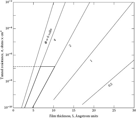
FIGURE 20.6
Tunnel resistance (φ is the work function) [1,2].

The next mechanical consideration involves the generation of friction-excited vibrations. This was considered from the standpoint of brushes by Shobert [10]. A machine was built in which a brush could be rotated about the point 0 in Figure 20.7 [10]. The brush had its heel cut away so that the point of application of the friction force would not change as the brush was rotated. It was found that brushes could and would chatter and whistle within the angular range θ, but that outside this angle on either side, the brushes could not chatter. The reason for this is shown in Figure 20.8. At the angle θ, the friction force is equal to the component of P tangential to the surface. At a slightly greater angle the tangential component P sin θ of the brush force P is greater than the friction force, μ P cos θ, so there is no backward motion of the brush and therefore no chatter. Where the friction force μ P cos θ is greater than P sin θ, vibrations are excited because there is a component of the vibration normal to the surface that provides the periodicity. The friction force μ P cos θ has a component μ P cos θ sin θ opposite to the direction of the force P that causes the brush to shorten elastically. This shortening decreases the normal force P cos θ that causes the friction force μ P cos θ to decrease. When μ P cos θ decreases, the brush force recovers elastically and the process is repeated. The brush then vibrates longitudinally at a frequency determining by its elasticity, length, and density.

At the limit where μ P cos θ = P sin θ, we may write

$\text{μ}=\tan \text{θ}$

(20.13)

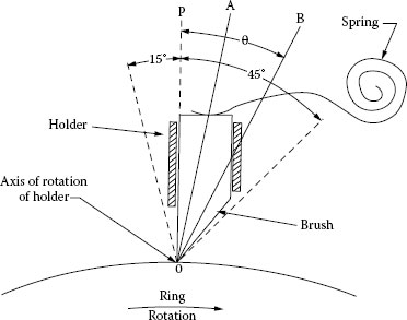
FIGURE 20.7
Schematic diagram of special brush holder. (From E.I. Shobert II, Carbon Brushes, New York: Chemical Publishing Co., p 62, 1965 [2].)

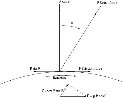
FIGURE 20.8
Chatter range.

and thus determine the maximum angular range θ within which brushes may chatter. If the force P is on the other side of the vertical, P sin θ and the friction force F are in the same direction, forcing the brush against the holder, and there is no vibration. The experimental results in Reference [10] show this to be the case.

Radial brushes have a tendency to chatter depending on which part of the apparent surface is making contact. Chatter is inhibited and prevented by designs in which the brush is held against one or the other sides of the holder by various bevels [11].

As for other aspects, a ring surface has roughness, and its influence on contact voltage drop is reported [12], and the relation between contact voltage deviation and ring profile distortion is made clear [13]. As mentioned before, the friction is one of the key factors, and the measurement methods of the dynamic of friction are reported [14].

We cannot over-emphasize the importance of the mechanical design on successful brush operation. The actual requirements are very rigid. The presence of suitable lubricants, moisture, and adjuvants, and the properties of the brush face make successful applications possible. It is important to know why brushes work so that in designing a machine or working on a problem, we know what the problem really is and not waste effort on something that will not be productive.

20.3  Chemical Aspects

Under chemical effects, we will consider the oxidation of the conductor surface, the presence of the moisture layer, the effects of other environmental or ambient materials, and how these relate to friction and conduction.

20.3.1  Oxidation

The question of film formation on metals has been discussed in several places previously in this book (see Chapters 1 through 3). In sliding contacts, we are concerned primarily with collector materials of copper and copper-based alloys, silver and silver alloys, and several of the precious metals, gold, platinum, palladium, for example. The copper-based alloys oxidize by the diffusion of the metal ions through the film so that the rate of oxidation decreases as the film develops. The same is true of silver in an atmosphere containing sulfur, except that without sulfur the electrical conducting area can increase beyond the area determined by “fritting,” and silver can act similarly to gold.

On the other hand, the rate of oxidation is influenced by the direction of the electric current. Since the oxidation proceeds by the migration of metal ions through the film, this will be enhanced under the cathode brush and impeded under the anode brush. This explains the fact that the voltage drop is usually higher for cathode brushes, although this may be reversed for metal graphite brushes.

When copper is machined, an oxide film several molecular layers thick forms quickly behind the cutting tool. Figure 20.9 [15] shows how copper oxidizes in relatively dry air. Figure 20.10 [16] shows the relative oxidation rates on different crystal faces of copper and Figure 20.11 [17] shows the effect of moisture in the air. Thus, we readily see that the oxide film alone is complicated. The addition of other atmospheric contaminants further complicates the result.

20.3.2  Moisture Film

As pointed out in the introduction to this chapter, the moisture film is the most important factor in the atmosphere affecting brush performance. The importance was first noted by Dobson [18] on rotary converters in the Chicago area where brush life was very short during the season of dry air in the winter. The problem was solved by releasing steam into the rooms when the humidity was low. The problem reappeared when high flying aircraft in World War II lost electric power when the brushes wore rapidly or “dusted.” This problem was solved by Elsey [19] who added metal halides to the brushes. PbI and BaF were the first to be considered. These had the drawback of requiring extensive run-in at sea level to develop a protecting film. MoS₂ solved this problem by providing a material that would protect immediately on running at altitude. It should be noted that many different materials have the same characteristic as MoS₂ to protect against this rapid wear, but that there are other requirements for brushes. These include long-term storage with the brush in contact with the collector in high humidity. Many corrode the collector or the brush holder.

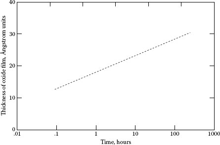
FIGURE 20.9
Oxidation of copper in air. (From U.R. Evans, The Corrosion and Oxidation of Metals. London: Edward Arnold, Table 1, p 53, 1960 [15].)

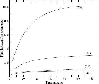
FIGURE 20.10
Oxidation of four faces of a copper single crystal at 178°C. H.C. Gatos, The Surface Chemistry of Metals and Semi-conductors, New York: Wiley, pp 486 ff., 1959 [16].)

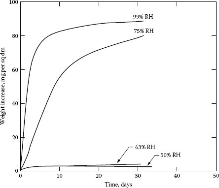
FIGURE 20.11
Corrosion of copper. (From W.H.J. Vernon, Trans Faraday Soc. 27:255, 582, 1931 [17].)

The above fact told us that moisture was the key, although it was later understood that other materials in the atmosphere could also prevent dusting. Oil vapors from the lubricants, smoke, organic vapors, any materials that could be quickly adsorbed on the collector could prevent the high wear. It was for these reasons that material tests had to be run under very clean conditions for consistent results.

The result, of course, is that brushes now operate in the vacuum of outer space for long periods. From a practical point of view the lower limit on moisture content can be taken as about −10°C dew point. While wear is somewhat variable around this point, catastrophic wear does not usually take place above this point.

We have seen that for friction, the friction force is given by (Equation 20.9),

$F=\text{ψ}{A}_b$

(20.14)

where Ψ is the shear strength of the film and A_b is the mechanical load-bearing surface. ψ is the result of the chemistry of the system and A_b is dependent on the mechanics.

It would appear that the shear strength of the film is governed in part by an effect similar to an activated adsorption in which the rate of adsorption at the surface varies with temperature, as shown in Figure 20.12 [20]. Figure 20.13 shows the general nature of the way that friction varies with temperature in graphite-lubricated contacts. As will be shown later, temperature depends not only on the ambient conditions but also on the microscopic situation at the contact face. When sulfide or silicone vapor is included in air, contact failure may happen owing to increasing contact resistance. As for silicone contamination, safe level of silicone vapor was reported [21]. In addition, the idea of vapor lubrication was successfully proposed to protect contacts from surface contamination from atmosphere [22].

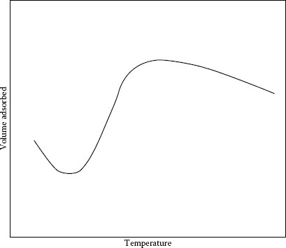
FIGURE 20.12
Activated adsorption. (From S. Glasstone, K.J. Laidler, H. Eyring. The Theory of Rate Processes, New York: McGraw Hill, pp 339 ff, 1941 [20].)

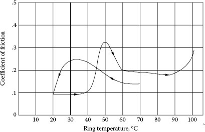
FIGURE 20.13
Coefficient of friction vs. ring temperature. Electrographite in air; dew point 14°C. (From E.I. Shobert II, Carbon Brushes, New York: Chemical Publishing Co., 1965 [2].)

For special application of brushes brush-ring systems are sometimes used in gases other than air [23,24].

When the possibilities are considered it is easy to see why many brush tests are out of control. As previously stated, each part of the system is affected by and depends on various aspects of the other variables so that all must be taken together in consideration of a particular problem.

20.4  Electrical Effects

While the purpose of a sliding electrical contact is to conduct current between moving and stationary contacts, this cannot be done successfully unless the mechanical and chemical aspects are proper. When they are in order we can review the electrical effects and see how they relate to the other phenomena. We are concerned here with the contact voltage drop, the tunnel effect, the fritting or electrical breakdown of the oxide or non-conducting films, and the commutation phenomenon.

20.4.1  Constriction Resistance

One of main elements of the contact drop is the constriction resistance within the brush. As shown by Shobert [2] the conducting surfaces on the face of the collector are sometimes long narrow lines. The resistance of such considerations can be approximated by the relation

$R=\frac{\text{ρ}}{2\text{π}l}\ln \frac{B}{b}\left(\text{ohms}\right)$

(20.15)

where

ρ is the resistivity of the brush;

l is the length of the conducting area;

B is a dimension similar to the width of the brush; and

b is the half-width of the conducting area.

This relation neglects the effects at the end of the conducting areas, but we are concerned with principles at this point. A further refinement would put a resistance of half of a “b” spot at each end of the strip or a resistance

$R_b=\frac{\text{ρ}}{4b}$

(20.16)

in parallel with that of Equation 20.15. As shown by Shobert [25] the conducting surface is influenced by the voltage direction and

$R_{\text{c}}~\frac{1}{l}$

(20.17)

under the cathode brush and

$R_{\text{a}}~\ln \frac{1}{b}$

(20.18)

for the anode brush. The other element of the contact drop or voltage drop in a sliding contact is the drop in the collector that is usually negligible except in the case of metal–graphite brushes with high-metal content.

20.4.2  Film Resistance

Then there is the drop in the moisture or other film. Since this film is insulating, (H₂O, CuO, MoS₂, etc.) as is required to prevent the electron clouds of the brush and collector from comingling, conduction takes place across this film by means of the tunnel effect. This is shown in Figure 20.14, in which it is seen that electrons with sufficient energy can “tunnel” through the potential barrier between the two surfaces. The effective resistance of this insulating film has been calculated by Holm as shown in Figure 20.6.

Figure 20.15 [25] shows the “B” fritting of a brush film on copper as probed with a gold wire. The test results in Figure 20.15 were taken on (a) an insulating region and (b) a conducting region of a carbon brush track with a gold wire. In Figure 20.15a “B” fritting is shown to occur around 0.3 V, while in Figure 20.15b, R-V characteristics are reversible. For comparison “B” fritting on an oxidized copper plate is shown in Figure 20.16 [1]. The temperatures were calculated on the same basis as those to be discussed in the next section.

In the case of a brush-ring sliding system, a voltage increase is observed just after the ring starts moving. As shown in Figure 20.17 [25] the increase value is relatively constant at about 0.3 V. Obviously, this additional voltage is caused by some film formed between moving ring and brush. The voltage between the brush and the ring at the edges of the tunnel effect film seems to be “B” fritting voltage, which is relatively constant and independent of the current for a copper collector and silver in the presence of sulfur. The voltage difference between stopped and running for electrographite brush on copper is about 0.3 V and the correlation is apparent. Thus the voltage drop can be summarized by Figure 20.18 [2].

We can now say that the conduction mechanism may be represented by Figure 20.18 where we have the constriction resistance in the collector, the voltage increase on sliding, and the constriction within the brush. Included in the equilibriums at low and high current is the effect of abrasives in the brush that will be discussed later. Important to note here is the fact that if the current is suddenly (60 Hz) reversed to zero and back as in the straight lines A and B, the resistance remains constant, indicating that the conducting area has not changed and that there is no semiconducting effect present.

20.4.3  Fundamental Aspects of Commutation

Large power dc motors used in steel plants, transportation vehicles, and other applications have been replaced by ac variable speed motors recently. However, small dc motors are widely used in various applications. Specially, many small dc motors are in automotive appliances. Approximately 30–40 motors are used in one automobile. Recently, the automotive electric power system is under consideration of changing from 14 V to 42 V power net. Supposing the 42 V power net, intensive research has been made [27,28,29,30].

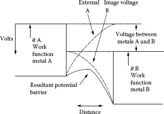
FIGURE 20.14
Schematic representation of the tunnel effect.

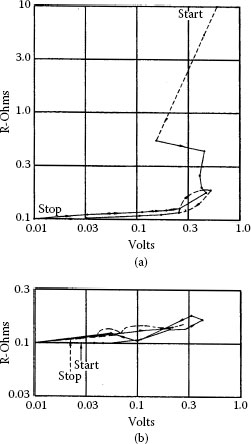
FIGURE 20.15
“B” fritting of copper oxide [25]: (a) insulating spot on the ring; (b) conducting spot on the ring.

Among automotive electromechanical devices, a dc motor has the feature that it is high in efficiency and easy to adjust its rotation speed by voltage of a power source. However, it has a sliding mechanism between commutator and brush, and arc discharge between brush and commutator segment is a big problem [31]. A commutation of the dc motor means that a coil current is reversed in its direction when the coil passes through neutral zone between magnetic poles.

At the termination of the commutation an arc discharge sometimes occurs, depending on commutation current, coil inductance and speed. Figure 20.19 shows a coil current distribution of the dc motor. In this case, a torque generates in counterclockwise direction. However, the armature coil rotates and the coil located around the magnetic neutral zone enters into the opposite magnetic pole zone. If the current direction of the coil remains unchanged, generated torque will be reversed in direction and the counterclockwise rotation cannot be continued. So, in order to keep counterclockwise rotation, the coil current should be changed in direction when it passes through the magnetic neutral zone. The current reverse is called commutation in a dc machines and Figure 20.20 shows how the commutation current changes its direction with time. The commutation current is expressed by Equation (20.19) during the commutation period.

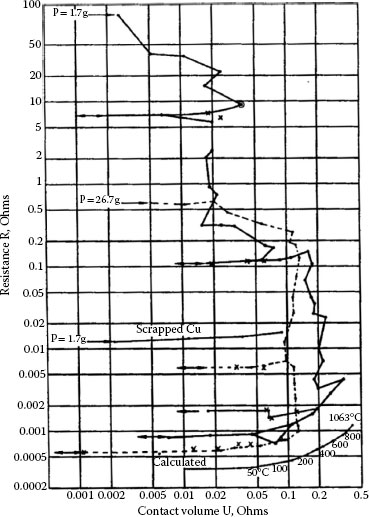
FIGURE 20.16
“B” fritting of copper oxide on copper rods. (From R. Holm, Electric Contact Handbook. Berlin: Springer-Verlag, pp 7–8, 1967 [1].)

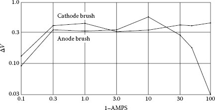
FIGURE 20.17
Voltage difference ΔV between stop and run as a function of current. (From E.I. Shobert II, Electrical resistance of carbon brushes on copper rings. IEEE Trans. Power, Apparatus and Systems, 13: 788–797, 1954 [25].)

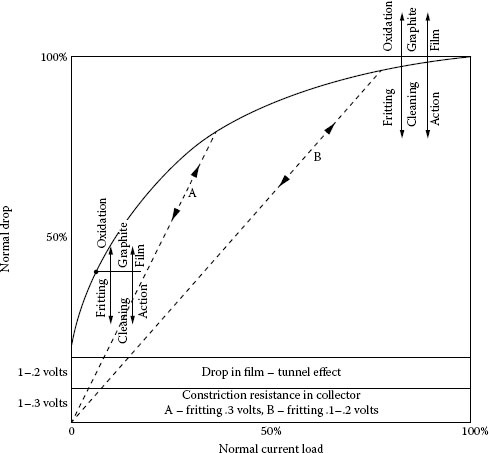
FIGURE 20.18
Schematic of brush voltage drop vs. current.

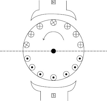
FIGURE 20.19
Coil current distribution of dc motor.

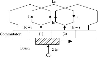
FIGURE 20.20
Commutation circuit of dc motor.

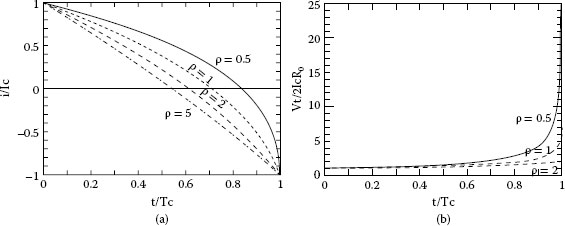
FIGURE 20.21
(a) Change of commutation current; (b) Change of trailing voltage $\left(\text{ρ}=L_c/R_0{T}_c\right)$.

$\begin{array}{l}{L}_c\frac{di}{dt}+R_1\left(I_c+i\right)-R_2\left(I_c-i\right)=0\\ R_1=\frac{R_0}{1-t/T_c},R_2=\frac{R_0}{t/T_c}\\ t=0,i=I_{c}andt=T_c,i=-I_c\end{array}$

(20.19)

where L_c: commutation coil inductance, i: coil current, I_c: armature coil current, R₁: trailing side resistance between brush and commutator segment, R₂: leading side resistance, T_c: commutation period, R₀: contact resistance at full contact between brush and commutator segment.

From (20.19), the coil current changes during the commutation period from I_c to −I_c as shown in Figure 20.21(a). As the commutation is progressing, the contact surface of the trailing side of the brush decreases, but the current change is delayed owing to the coil inductance L_c. Consequently the current density of the trailing side becomes high, and the contact voltage drop v_t is increasing (see Figure 20.21(b)). The temperature of the contact area is rising, and reaches a threshold value (usually, boiling voltage in case of metal and sublimating voltage in case of carbon). Finally, metallic contact between brush and commutator segment is broken. At that time, the current still flows through the brush and segment that is called a residual current. If the residual current is larger than the minimum arc current, an arc discharge will occur when the brush leaves the segment. This model is shown in Figure 20.22.

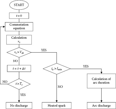
FIGURE 20.22
Calculation model of commutation arc.

20.4.4  Equivalent Commutation Circuit and DC Motor Driving Automotive Fuel Pump

Generally an actual dc motor should be used to investigate its performance. However, in an actual dc motor, it is difficult to measure the duration of arc discharge and commutation current. So, an equivalent commutation circuit. was proposed. It represents only the commutation process of the dc motor in terms of an electrical circuit. Figure 20.23 shows an equivalent commutation circuit [32,33]. Among many dc motors used in a car, a motor driving a fuel pump has a unique feature that the commutation is carried out in gasoline. We have been much interested in the commutation in gasoline and its influence on commutator and brush. Figure 20.24 shows typical voltage and current waveforms during the commutation. The final stage of the commutation is enlarged, and the voltage between brush and commutator segment abruptly increases and an arc discharge is established. As a feature of arc voltage, the voltage value in gasoline is higher than in air [33].

20.4.5  Arc Duration and Residual Current

Figure 20.25 shows an equivalent circuit when an arc occurs between brush trailing edge and segment. The circuit equation is expressed as follows;

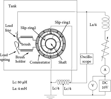
FIGURE 20.23
Equivalent commutation circuit.

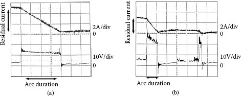
FIGURE 20.24
Voltage and current waveforms. (a) In air; (b) In gasoline.

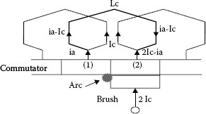
FIGURE 20.25
Commutation circuit during arc.

$L_c\frac{d\left(I_c-i_a\right)}{dt}+R_c\left(I_c-i_a\right)+R_0\left(2I_c-i_a\right)-v_a=0$

(20.20)

where R_c is a resistance of the commutation coil and i_a and v_a are arc current and arc voltage, respectively.

As the initial condition is i_a = I_e, (residual current) at t = 0, the solution of (20.20) is obtained as follows;

$i_a=\left(I_e+K\right)\exp \left(-\frac{t}{T}\right)-K$

(20.21)

where $K=\frac{v_a+\left(R_c-2R_0\right)I_c}{R_c+R_0},T=\frac{L_c}{R_c+R_0}$

As the arc distinguishes at i_a = I_min (minimum arc current), the arc duration is expressed by;

${\text{τ}}_a=T\ln \frac{I_e+K}{I_{\min }+K}$

(20.23)

If $\frac{{\text{τ}}_a}{T}\ll 1$ and $K\simeq \frac{v_a}{R_c+R_0}$, the arc duration (20.22) is simply reduced to the followings;

${\text{τ}}_a=\frac{L_c}{v_a}\left(I_e-I_{\min }\right)$

(20.23)

Figure 20.26 shows the relation between residual current and arc duration that are experimentally obtained in air and gasoline. From these results, the arc duration is almost proportional to the residual current as predicted by (20.23). On the other words, the Equation 20.23 is simple but useful [33].

In most machine designs, particularly in cases where the machines are made in large production quantities, the effort is made to use materials and processes to their economic limits. This results in problems that usually result in short brush life or related difficulties. To solve these problems it is necessary to understand all of the factors that are effective in successful operation and to see where deviations from the ideal take place. Again we are dealing with complicated situations where mechanical, chemical, electrical, thermal, and material problems are concerned.

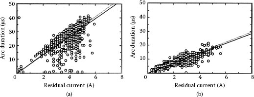
FIGURE 20.26
Arc duration vs. residual current Arc. (a) In air; (b) In gasoline.

20.5  Thermal Effects

Thermal effects in stationary contacts are discussed in Chapter 1. The basic principles for sliding contacts are similar, with the addition of friction heating which takes place over the mechanical sliding surface and transient phenomena which appear because the mechanical and electrical contact spots are moving to different positions on the collector and the conducting regions on both the brush and collector are elongated in the direction of motion.

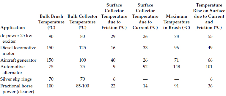
From the standpoint of knowing how to analyze various problems of brushes, however, it is important to know the maximum temperature in the brush and the temperature at the surface of the collector. These have not been measured directly, but there are means to calculate them with sufficient accuracy for most purposes. These calculations involve, first, calculating hypothetical steady-state temperatures generated by both the friction and the electrical heat, and then applying a time-dependent factor that indicates what parts of these hypothetical temperatures are reached. Examples of these calculations and the details of the formulas are given in Shobert [2], in the chapter on brush temperatures. They are summarized here and several examples of the results are shown in Table 20.2.

Certain essential ideas of the contact theory provide the basis for these temperature calculations. These include the calculation of the mechanical sliding surface from the hardness of the brush materials, the calculation of the electrical contact surface from the voltage drop and the specific resistance of the brush materials, a preliminary calculation of the hypothetical steady state temperatures owing to friction and current—assuming that the contact surfaces have time to come to equilibrium—and then the calculation of the fraction of the steady-state temperature that is actually reached during the available time of contact while the contact spots are passing under the brush.

20.5.1  Steady State

The friction heat is generated over the mechanical contact surface, which is of the order of 1% or less of the apparent brush surface. Because the hottest isotherm is always located in the brush, it is assumed that all of the friction heat goes to the collector and causes a hypothetical steady-state temperature rise (ϑ_f) where

TABLE 20.2
Brush Temperatures (Kohlrausch–Holm Method)

$\left({\vartheta }_{\text{f}}\right)=qW{b}_1\left({}^{\circ }\text{C}\right)$

(20.24)

and where q is the friction heat current and $W_{b_1}$ is the thermal resistance within the collector of the constriction pertaining to the mechanical contact area on the collector surface. For one circular contact area, A_b,

$W_{b_1}=\frac{1}{4\text{λ}{b}_1}\left({}^{\circ }\text{C}{\text{/W}}^{-1}\right)$

(20.25)

where λ is the thermal conductivity of the collector and b₁ is the radius of A_b. This surface A_b is

$A_b=\text{π}{b}_1^2=\frac{P}{H}\left({\text{cm}}^2\right)$

(20.26)

where P is the brush spring force and H is the contact hardness, about two-thirds the hardness as defined by ball indentation tests (see Figure 20.4).

Next, we calculate the hypothetical steady-state temperature rise of the collector surface and of the maximum temperature in the brush (see Figures 20.27 and 20.28). From the consideration of the unsymmetrical contact, we have the equations, which are derived in [2], but which are listed here for reference:

$V^2=Z{\text{ρ}}_1{\text{λ}}_1\left(\text{θ}-\vartheta \right)\left({\text{V}}^2\right)$

(20.27)

and

$u^2=2{\text{ρ}}_1{\text{λ}}_1\text{θ}\left({\text{V}}^2\right)$

(20.28)

where now V is the voltage from the brush face to the point of maximum temperature in the brush, u is the voltage from the point of maximum temperature in the brush to the bulk of the brush, ρ₁ is the resistivity of the brush materials, and λ₁ is the thermal conductivity of the brush material. For simplicity, ρ₁ and λ₁ are considered in these calculations to be independent of the temperature. While involving an approximation, this is permissible since the steady-state super temperatures are fictitious quantities which never appear, and the values of ρ₁ and λ₁ near the bulk temperature of the brush and collector are suitable in the light of some of the other assumptions and approximations. ϑ is the steady-state surface super temperature of the collector, and θ is the steady-state maximum super temperature in the brush. ϑ and θ are related by the expression

$\vartheta =\frac{4{\text{λ}}_1\left({\text{λ}}_1+\text{λ}\right)}{\left({\text{2λ}}_1+\text{λ}\right)}\text{θ}\left({}^{\circ }\text{C}\right)$

(20.29)

We also find that

$\Phi V=\text{ρλ}\vartheta \left({\text{V}}^2\right)$

(20.30)

where Φ is the voltage drop in the collector, which is usually small compared with V + u, the voltage drop in the brush.

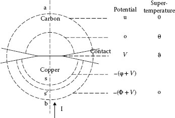
FIGURE 20.27
Relation of voltage and temperature in the asymmetric contact.

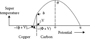
FIGURE 20.28
Temperature vs. voltage in the asymmetric contact.

The voltage will be distributed approximately proportionally to the average resistivities since the electrical conducting surface is the same for both the collector and the brush. We may therefore write

$\frac{\text{Φ}}{V+u}=\frac{\text{ρ}}{{\text{ρ}}_{\text{1}}}$

(20.31)

if ρ and ρ₁ are averages within the temperature ranges.

The voltage V + u represents, in most practical cases, the measured voltage brush drop. Thus from Equations 20.27, 20.28, 20.30, and 20.31, we can calculate ϑ and θ. Equation 20.28 can be used as a check on the calculations. It should also be noted that the tunnel resistance is considered a part of V + u.

These stationary temperatures are not reached because any contact spot is active for too short a time to reach thermal equilibrium. The general equation for the time rate of heating in a volume element is

$\text{λ}{\nabla }^2\vartheta +\text{ρ}{J}^2=C\frac{\text{d}\vartheta }{\text{d}t}\left({\text{W/cm}}^{-3}\right)$

(20.32)

where J is the current density and C is the heat capacity of the materials. Holm [1] gives solutions of this equation for circular contact spots. The solutions are represented by diagrams, in which the time is replaced by the dimensionless variable

$z=\frac{\text{λ}}{{\text{cb}}^2}\text{t}$

(20.33)

The solutions we shall use are shown in Figure 20.29a, in which the fraction of the steady-state temperature that is reached is plotted as a function of z. In Figure 20.29, ϑ_f, ϑ_s, and θ_s represent the part of (ϑ_f), ϑ and θ that appears in the transient period. It is assumed that the temperature rise owing to the friction heat, ϑ_f, can be added to the other temperature rises to give the total temperature rise on the surface ϑ_v, and the maximum temperature rise in the brush θ_v. Thus,

${\vartheta }_{\text{v}}={\vartheta }_{\text{f}}+{\vartheta }_{\text{s}}\left({}^{\circ }\text{C}\right)$

(20.34)

and

${\text{θ}}_v={\vartheta }_{\text{f}}+{\text{θ}}_{\text{s}}\left({}^{\circ }\text{C}\right)$

(20.35)

20.5.2  Actual Temperature

We now come to the crux of the problem, which involves the determination of the values of b and t under the circumstances involved in sliding brush contacts. We calculate t as t_v from the relation

$t_{\text{v}}=\frac{\text{π}{b}_1}{2v}k$

(20.36)

where b₁ is chosen for the mechanical contact surface (assumed to be a single circular area), v is the velocity of the moving surfaces, and k was arbitrarily given the value 5. k represents an effective elongation of the surfaces in the direction of motion, which has been shown to exist [25], but the value 5 is purely an educated guess. Placing t_v from Equation 20.36 and b₁ from Equation 20.25 in Equation 20.32, the proportion of (ϑ_s), which appears at the collector surface, can be calculated from Figure 20.20a and we thus have ϑ_f, the temperature rise on the contact surface owing to friction.

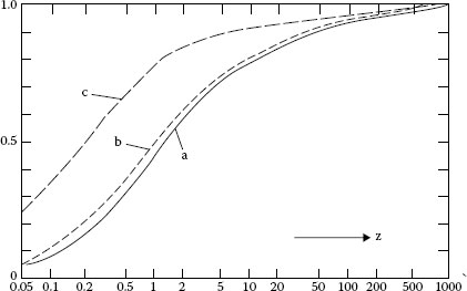
FIGURE 20.29
Correction for transient effects in brush and collector applications: (a) ϑ_s/ϑ for collector surface; (b) ϴ_s/ϴ for maximum temperature in brush; (c) ϑ_f/(ϑ_f) for temperature rise at surface owing to friction.

The calculation of the value of b in Equation 20.33 for the case of electrical heating requires an assumption concerning the number n of electrically conducting contact spots operating in parallel. Here again, purely arbitrary choices are made.

The choices of k = 5 and n = 10, although arbitrary, have reasonable basis on other areas of general experience. However, in any particular problem the basis must be noted and the data considered in this light.

From a design standpoint, there are several factors that should be considered. Since the maximum temperature occurs back in the brush, the heat flow of about half of the electric heat is from the brush to the collector. Also the heat flow from the mechanical surface, owing to friction, is distributed between the brush and collector approximately in proportion to their thermal conductivities. This only emphasizes the importance of the collector in getting rid of heat. It also points out that where the limits are being stretched for increased currents and speeds, the overall heat flow and dissipation must be considered.

20.5.3  Thermal Mound

Another factor considered for applications, which are stretching the limits on current and speed is thermal mounding. This is a raised region that expands from both surfaces owing to the temperature rise in the current constriction and owing to friction. Particularly for high-current and high-speed application, this mounding can force the current to be transmitted in very few contact spots. The wear is concentrated on an individual spot until it wears away and the current and friction are transferred to another spot. The height of these mounds can be very small considering the film thickness of 10⁻⁷ for the water film. Bryant and others have calculated the temperatures and extensions of this mounding [34,35,36,37]. Practical observations on machines where selective action is taking place point to the fact that when brushes become overloaded, the number of contact spots under the brush decreases. This sometimes ends in glowing, that is, a bright glow on the trailing edge of a brush that moves slowly across the width.

20.6  Brush Wear

Brush wear is the resultant of the several processes involved in brush operation. Low rates are required on power machines and satellite rings while high rates are permissible on torpedo motors. It is always possible to decrease wear rates by more conservative design, but successful designs balance wear rates to the economic requirements of the application.

We shall consider as a measure of wear the change in length of the brush or slider divided by the length of the path on the collector over which it has slid. On this basis Shobert [38] has placed the wear of brushes in the general context of mechanical wear, as shown in Figure 20.30, in which rates of wear are shown with respect to the ranges of the coefficients of friction for a variety of sliding systems, from the oil-lubricated sleeve bearing to chalk on a chalkboard. The wear rates cover about 14 powers of ten, whereas the friction extends over 3 powers of ten. The reason for presenting this schematic diagram is to point out that all the phenomena of wear cannot be lumped together and considered as being the result of the same physical effects. The wear of chalk on a blackboard results from the fact that the coarse asperities on the board are stronger than the chalk. Shear takes place within the chalk, leaving dust held to the board by weak cohesive forces that can be broken when the soft felt of an eraser rubs into these asperities. In fact, the wear and crumbling of chalk are so drastic that only a part of the dust sticks to the board.

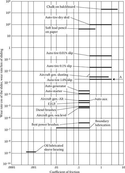
FIGURE 20.30
Schematic representation of friction and wear.

By contrast, the wear in an oil-lubricated sleeve bearing is caused by the incidental touching of metallic asperities on the metal surfaces. These are held apart for the most part by pressure of the liquid that has been drawn into the load-bearing contact by the adhesion between the liquid and the two surfaces.

Generally brush wear has the following three types.

1.  Mechanical wear with no load current

2.  Mechanical wear with load current

3.  Electrical wear (by arc discharge etc.)

Further, the mechanical wear is classified into the following two types;

1.  Adhesive wear

Material is dropped off by shearing or rupturing the adhesive contacts (see Figure 20.31).

2.  Abrasive wear

This is produced when asperities and particles attached to one contact member cut into the other member and form grooves.

It is interesting to note that on the best power brushes (on large generators in a steel mill), the wear is only two powers of ten higher than that of oil-lubricated bearings. Such brushes have an estimated life of about 4 years. The high rate of wear on brushes on aircraft or space vehicles, known as dusting, is only three powers of ten above that found in normal sea-level machines; and suitable brush materials have been designed to prevent this dusting as had been discussed above.

In Figure 20.30, the arrow on the right represents a rate of wear such that a brush with a face 1 cm thick in the direction of motion would leave one layer of carbon atoms on the collector surface as it passed over it once. The brush application with the highest wear has 1/10 this rate, and the lowest has 1/10,000 of it. In addition, it is to be understood that the wear particles are not individual atoms but are small particles of material that may contain some 10¹² atoms (particles with linear dimensions of 1 × l0⁻⁴ cm). If the particles were this large, there would be 10,000 left on every square centimeter of the track for wear corresponding to the point A, or 1,000 per square centimeter for the automotive generator. On the same basis, there would be one particle every 10 square centimeter on the track of the collector under one of the best power brushes.

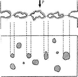
FIGURE 20.31
Contact surface model.

Of course, the wear debris is not as uniform as in the picture given in the previous paragraph. There is a wide spread in the size of the wear particles and, in addition, only a very small part of the total wear debris adheres to the collector track. In fact, some machines wear out many sets of brushes without building up excessive graphite films, indicating that an equilibrium must be reached very early on a new collector surface, in which the wear of the materials from the collector is just equal to the amount deposited, and no further accretion of carbon occurs.

Under normal conditions, then, we may consider the wear of brushes to be the result of the occasional contact between surface asperities.

The general subject of mechanical wear has been treated by Holm.

It has been pointed out that there can be a difference of three orders of magnitude in mechanical brush wear on commutators. The higher rates of wear could be reduced by improving the mechanical design, but in some cases such improvements would not be justified on economic grounds. Wear is usually increased when current is being carried, and as there is nothing about the passage of current through a normal contact which, by itself, should cause wear, the wear must be because current produces changes in the topography of the surfaces.

20.6.1  Holm’s Wear Equation

The electrical wear owing to arcing and sparking, as such, is very low; but the resulting disturbance to the commutator and brush surfaces can result in high brush wear.

R. Holm proposed an equation of wear under the conditions of current and arc discharge [39].

$W=P\left[W_{\text{o}}+C_1\left\{\text{τ}\left(2\right)+2\text{τ}\left(5\right)\right\}I+g\sqrt{Q}\right]+\text{ω}Q{\text{cm}}^3/\text{km}$

(20.37)

where P: mechanical load on a brush, I: current per brush, Q: electric charge transported by arcs during 1km of sliding, ωQ: volume evaporated from the brush under the influence of the arcs, τ(2), τ(5): fractions of the test time during which the voltage is over 2 and over 5 V respectively, the number 2 before τ(5): weight to the wear compared with τ(2).

Each term means that PW_o: wear without current, $P{C}_1\left\{\text{τ}\left(2\right)+2\text{τ}\left(5\right)\right\}I$: wear owing to surface roughening by the flashes, $Pg\sqrt{Q}$: wear owing to surface roughening by arcing where the square root is motivated by earlier measurements and g is a coefficient that is determined so as to provide optimum agreement between formula and measurements.

In the above equation, the rate of brush wear is a function of the number and duration of arcs, defined as discharges in which the voltage drop of the cathode is 12–20 V; and the number and duration of so-called “flashes,” in which the voltage does not reach 10 V. By placing an auxiliary brush on the commutator next to the normal brush and applying the brush voltage across a gated counter, the number of pulses of over 2 V, over 5 V, and over 10 V could be counted. From these numbers, and from the durations measured with an oscilloscope, the total time of the arcs as well as of the flashes could be calculated.

Figure 20.32 shows an oscillogram of such pulses; the lines show the voltages at which the counter was set. The wear caused by the short arcs was found to be smaller than the wear caused by the flashes. The relatively small influence of the short arcs is owing to their very short duration. The arcs usually form at the trailing edges of both brush and bar, and thus their duration is determined only by the residual inductive energy in the commutation coil. The flashes are usually generated under the brushes and can continue until the bar leaves the brush.

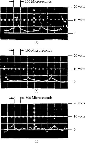
FIGURE 20.32
Oscillogorams of arcing, sparking, and flashes: (a) long arcs 20–60 ms (arcing); (b) short arcs 2–5 ms (sparking); (c) flashes 100–300 ms (over 2 V).

20.6.2  Flashes and Smutting

As the normal brush contact drop is of the order of 1–1.5 V, the higher voltage that appears during the flashes goes into heating of the region in both brush and commutator surfaces at and near the original conducting spots. These flashes are the result of mechanical circumstances, which cause enough loosening of the contact between the two surfaces to increase the resistance and therefore the voltage, but do not cause the complete separation that would lead to arcing. The temperatures in the conducting spots in both surfaces can be high enough to melt and even boil copper or, in longer flashes, to vaporize carbon. According to Holm [40] a flash of 4 V heats the copper surface to about 450°C. A flash of 6 V raises this temperature to about 900°C. In fact, this evaporation is very likely to be the cause of the “smutting” which appears on certain commutators when the machines are subject to excessive vibration or when the mechanical contact is disturbed for any reason.

This smutting, which is a heavy, dull black film, can appear irregularly over the face of the individual bars or over irregular area of the commutator and, in turn, causes a change in friction in the areas on which it appears. Occasional interruptions or flashes cause no trouble because the normal cleaning action of the brushes eliminates the excess carbon as fast as it appears. If the amount is excessive, the smut increases beyond the ability of the cleaning action to eliminate it. Smutting is dangerous because in most cases it leads to more serious commutator deterioration, with resulting high brush wear.

There is a certain limit of recovery from smutting for any given combination of brush and machine. Two equilibria are involved, in one of which fritting and oxidation oppose each other, and in the other filming and cleaning action oppose each other. Smutting adds to the effects of oxidation and filming, and when it occurs, cleaning action must be increased.

20.6.3  Polarities and Other Aspects

On slip rings on which brushes of different polarities slide on separate tracks, a difference between the tracks becomes apparent. Under the anode brush, the graphite film develops more uniformly; oxidation of the collector is inhibited by the direction of the current, and fritting of the film takes place at a lower voltage. The surface under the anode brush is thus not disturbed as much as the one under the cathode brush; as a result, the brush life may be several times higher.

Under the cathode brush, oxidation is enhanced, the oxide film tends to grow thicker, and there is less graphite deposited in it. Hence, as fritting must take place at a somewhat higher voltage, there is more disturbance of the areas near the conducting regions and therefore more brush wear. This effect of oxidation and fritting on wear is even more noticeable in the very long life of brushes running in hydrogen. It is interesting to note that in tests on metal graphite brushes reported by Hessler [41] the anode and cathode wear rates are reversed. The presence of metal in the brushes very probably accounts for the difference, because this metal can now become oxidized.

The brush wear is affected by various factors, and many papers have been reported [42]. Among them, there are papers concerning the effect of PV factor (product of contact pressure and peripheral speed) on the wear, relation between contact resistance and wear, the influence of vibration and surface waviness on the wear [43,44,45,46].

The atmosphere surrounding the brushes has an important influence on the rate of brush wear. Baker [47] showed that brushes running in H₂, N₂ and CO₂ had much lower rates of wear than brushes operating in O₂. This was particularly true for the negative brushes under which oxidation is enhanced. In the absence of O₂, the surface was less disturbed by oxidation and fritting and the wear rate was much lower. In addition the wear of copper fiber brush in carbon dioxide environment was reported [48]. Further, the wear of brush in various fuels, gasoline, ethanol and others has been examined recently [49,50,51].

20.7  BRUSH MATERIALS AND ABRASION

The experience of writing with a lead pencil or dusting a stubborn lock with graphite powder would lead one to believe that pure graphite should be the ideal brush material. But it is not. Graphite made by heating petroleum coke to temperatures about 2500°C, or pyrolytic graphite made by depositing carbon on active surfaces about 2500°C from carbon containing gases, and natural graphite, mined in Sri Lanka, Madagascar, and Mexico, show the largest crystals in their structures. However, none of these alone has provided a suitable brush.

Brushes that work on actual machines all contain certain abrasives. This leads to the idea that these abrasives are necessary to polish the collector surface to a fine enough finish so that the thin film of water (10⁻⁷ cm) can be effective.

20.7.1  Electro- and Natural Ggraphite Brushes

It is interesting to note that most electrographitic brushes are made using lampblack as a base. Figure 20.33 shows a schematic of the general process. In such a series of operations, it can readily be seen that there is a lot of art as well as science involved.

The important point is that with lampblack as the base, the crystal growth of the graphite is limited and the edges of many crystallites are available as abrasives to provide the mechanical strength to smooth down the roughness of the collector and to provide the electrical conductivity. Table 20.3 shows the physical properties of some of the generic types of brush materials. The physical properties are those required by different applications, as shown in Chapters. 21 and 22, but the different forms of carbon provide the proper sliding surface.

The natural graphite materials contain an appreciable amount of ash (SiO₂, CaO, etc.) and they are usually used in combination with metals (metal graphite) or resins.

From the viewpoint of crystallography, the carbon atoms of the graphite are held within the layer planesby homo-polar bonds, and in fact the bonding of a carbon atom in these planes is stronger than the bond in diamond (Fig. 20.34). On the other hand, the bond between the layer planes is due to van der Waals’forces which are much smaller. Further evidence of this effect is that the electric and thermal conductivities of pure single graphite crystals are very high in the direction of the layer planes, but very low perpendicular to them. The ratio had been shown to be as high as 100,000 to 1.

However, since carbon does not melt, during ordinary process of graphitization the crystal growth is limited by the way in which the original carbon was formed. The wide variation is illustrated by materials such as charcoal, which is different from different kinds of wood, lampblack, which comes from burning oil without enough oxygen, carbon black, the same from gas, and the limitless possibilities of charring various organic materials—resins, plastics, coconut shells, etc. This divergence in the end results is a distinct advantage in the field of the brush applications, as a wide variety of combination of the various properties can be made possible [52].

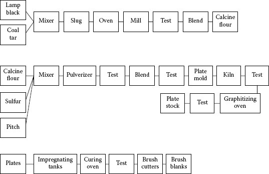
FIGURE 20.33
Typical process for the manufacture of electrographite brushes.

TABLE 20.3
Brush Materials

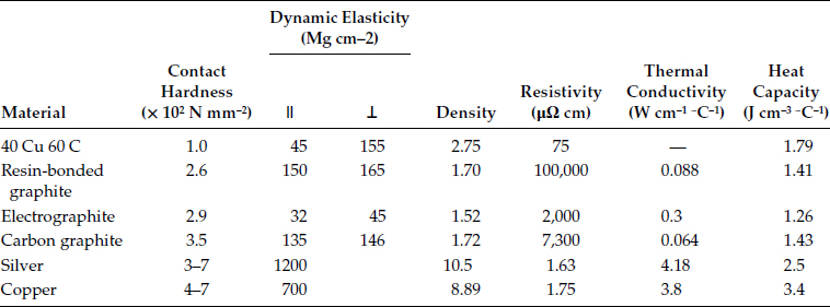
‖ or ⊥ refers to the direction of the measurement with respect to the molding pressure.

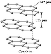
FIGURE 20.34
Layered structure of graphite atoms.

20.7.2  Metal Graphite Brush and Others

Metal graphite brushes can be made by the ordinary powdered metal processes, or by processes using plastic molding techniques. These give another dimension to the applicability of brush materials.

Metal graphite brushes are suitable for a variety of applications because of their low resistivity. For examples, metal graphites are used on commutators of plating generators where low voltage and high brush current densities are encountered. They operate on rings of wound rotor induction motors where high brush current densities are also common. Metal graphites are used for grounding brushes because of their low contact drop.

For the metal-graphite brushes low contact drop is obtained for more content of metal, whereas the wear becomes large with high content of metal [53].

Recently, monolithic and metal/metal coated fiber brushes were developed for high velocity and high current applications [54,55,56,57]. In addition, from the environmental issues lead-free carbon brushes have been developed [58,59]. Further, in the railroad system copper-impregnated carbon fiber reinforced carbon composites are developed for pantograph contact strips [60].

The important factor which goes through all of the considerations is the effects and the necessity for abrasion. It is carried out by the edges of small carbon crystals or by metals or by added materials such as sand. With the proper amount of abrasive, a collector which may have many mechanical, electrical, chemical and thermal flaws can be kept operating for suitable periods.

20.8  Summary

Sliding mechanism has been used to transmit electric power or signal between stationary devices and moving devices for over 100 years. Recently, transmission mechanisms without mechanical contacts have been developed on the basis of transformer principle and others. However, brush–slip-ring systems are still widely used in the aerospace, commercial/industrial, wind turbine and other applications, because of high transmission efficiency and simple structure, while with mechanical contacts their reliability and lifetime are important issues. In order to realize high reliability and long lifetime, various components must be considered in working with sliding contacts. They are all—mechanical, chemical, electrical, thermal, abrasion, and wear—interconnected in any brush application. The followings are a summary of this chapter.

1.  The progress of surface analysis methods can enable us to observe surface morphology in details (3D laser microscope) and to identify products on the contact surface (Auger electron spectroscopy, Atom force microscopy and others). In addition, electromagnetic analysis and linear or nonlinear stress analysis by FEM are also very powerful to know current distribution and micro deformation around contact surface. They are very useful tools for research and development.

2.  Mechanically, the sliding contacts ride on a thin film—water usually—which is only some few molecular layers thick. This places the mechanical system under constraints to permit this to happen. Without this film, brushes wear catastrophically. Water may be replaced by laminar compounds such as MoS₂, WS₂ and others, for operation in dry atmospheres, at high altitude, or in space.

3.  The mechanical contact surface is determined by the spring force and the contact hardness of the material. This may be divided into several regions scattered and moving around under the brush. At load bearing areas, elastic penetration of the collector into the face of the brush provides the ability of the face of the brush to accommodate small variations in the collector surface. This operates much faster than the whole brush that can move under the force of the spring, thus satisfying condition (2).

4.  Under high current and high speed, thermal mounds are formed in the contact surface. In that case the current is concentrated in the thermal mounds and the temperature of the thermal mounds becomes very high, so that the wear rate becomes very high.

5.  Under certain circumstances, brushes may squeal or chatter like chalk on a blackboard. This possibility can be eliminated by keeping the brush angle out of the range of possible chatter or by using suitable mechanical designs.

6.  In dc motors, the commutation is one of the important factors to their performance and lifetime. The commutation is a complicated phenomenon including electrical, mechanical and material aspects, and commutation arc is predominant to the lifetime. Its duration time τ_a is obtained from residual current I_e, commutation inductance L_c and arc voltage v_a by the following equation; ${\tau }_a=\frac{L_c}{v_a}\left(I_e-I_{\min }\right)$.

7.  Electric current differences built into the machine such as more than one coil per slot, differences in the resistance of armature windings, errors in armature coil turns, and eccentricities of the armature iron can cause exceptional currents at specific commutator bars. This usually leads to bar burning and the resulting short brush life.

8.  Wear particles tend to abrade the collector and the face of the brush. There are many, but they are small, and they contribute to the fine smoothing of the collector. The strength of the homopolar bond in the layer planes of carbon provides the fine abrasive which keeps the surface smooth and permits a certain deviation from uniformity in current at different parts of the collector. Other materials may also be added to the brush to provide additional abrasion.

9.  Fiber brushes have many distinct and measurable advantages over conventional slip ring contacts, that is, multiple points of ring contact per brush bundle and so low dynamic contact resistance (noise). Although much of the research have been on their use mainly for large current and high speed applications there is an interest in using these brushes at lower currents (see Chapter 23). Research does continue on carbon based sliding contact at high current for efficient railroad pantographs to carry current from overhead lines to high speed electric locomotives [60,61].

In a particular application, one or more of mechanical, chemical, electrical and thermal effects may dominate. It is then necessary to evaluate which is effective and work on the solution, considering materials. The fact that several may be operating together complicates the problem but proper analysis will usually permit a solution. Brush applications are usually a compromise in which cost, performance and life are balanced.

References

1.  R. Holm, Electric Contact Handbook. Berlin: Springer-Verlag, pp 7–8, 1967.

2.  E. I. Shobert II, Carbon Brushes, New York: Chemical Publishing Co., p.25, p.27, p.66, 1965.

3.  M. F. Gomez, Characterization and Modeling of Brush Contacts, Ph.d Dissertation, University of the Federal Armed Forces Hamburg, 2005.

4.  H. Tanaka, NMorita, KSawa, TUeno, Carbon brush and flat commutator wear of DC motor, driving automotive fuel pump in various fuels, Proc. of the 56th Holm Conf. on Electric Contacts, 2010.

5.  A. E. Bickerstaff, The Real Area of Contact between a Carbon Brush and a Copper Collector, Holm Seminar on Electric Contact Phenomena, 1969.

6.  S. Tsukiji, SSawada, TTamai, YHattori, KIida, Direct observation of current density distribution in contact area by using light emission diode wafer, Proc. of the 57th Holm Conf. on Electric Contacts, 2011.

7.  R. Holm, EHolm, E.I. Shobert II, Theory of hardness and measurements applicable to contact problems. J Appl Phys 20:310, 1949.

8.   RHolm, Friction force per unit area at true contact surface. Wissenschaftliche VeroffentLichungen a.d. Siemens-Werke 17(4):38, 1938.

9.  S. Sasada, SNorose, HMishina, The behavior of adhered fragments interposed between sliding surface and the formation process of wear particles, Trans. ASME, J Lubrication Technology, 103: 1981.

10.  E. I. Shobert II, Carbon brush friction and chatter, IEEE Trans Power Apparatus and Systems, 30:268, 1957.

11.  J. L. Johnson, Brush Mechanical Support Characteristics in Inclined Holders, Holm Seminar on Electric Contact Phenomena, 1970.

12.  T. Ueno, KKadono, N. Morita, Influence of surface roughness on contact voltage drop of electrical sliding contacts, Proc. of the 53th Holm Conf. on Electric Contacts, 2007, IEEE.

13.  M. Takanezawa, HYanagisawa, TUeno, NMorita, TOtaka, DHiramatsu, Brush sliding contact voltage deviation analysis based on the evaluation of displacement excited vibration caused by collector ring profile distortion, Proc. of the 54th Holm Conf. on Electric Contacts, 2008.

14.  M. Milkovic, Test methods and measuring apparatus for measurement of the dynamic coefficient of friction of brushes, Carbon, 30(4): 587–592, 1992.

15.  U. R. Evans, The Corrosion and Oxidation of Metals. London: Edward Arnold, 1960, Table 1, p 53.

16.  H. C. Gatos, The Surface Chemistry of Metals and Semi-conductors, New York: Wiley, 1959, pp 486 ff.

17.  W. .H.J. Vernon, Trans Faraday Soc. 27:255, 582, 1931.

18.  J. V Dobson, The effect of humidity on brush operation. Electric J, 32:527, 1935.

19.  H. M. Elsey, Treatment of high altitude brushes by application of metallic halides. AIEE Paper No. TP45–108, June, 1945.

20.  S. Glasstone, KJ Laidler, HEyring, The Theory of Rate Processes, New York: McGraw Hill, 1941, pp 339 ff.

21.  T. Tamai, Safe levels of silicone contamination for electrical contacts, Proc. of the 39th Holm Conf. on Electric Contacts, 1993.

22.  S. Uda, THigaki, HFunami, KMano, The general idea of vapor lubrication system applied in small power motors, Proc. of the 39th Holm Conf. on Electric Contacts, 1993.

23.  J. L. Johnson, JL McKinney, Electrical power brushes for dry inert-gas atmospheres, Holm Seminar on Electric Contact Phenomena, 1970.

24.  T. Ueno, NMorita, KSawa, Influence of surface roughness on voltage drop of sliding contacts under various gases environment, Proc. of the 49th Holm Conf. on Electric Contacts, 2003.

25.  E. I. Shobert II, Electrical resistance of carbon brushes on copper rings. IEEE Trans. Power, Apparatus and Systems, 13: 788–797, 1954.

26.  R. Holm. Electric Contacts, New York: Springer-Verlag, 1967, Fig. 27.13, p 147.

27.  N. Ben Jemaa, LLehfaoui, LNedelec, Short aec duration laws and distribution at low current (<1A) and voltage (14-42VDC), Proc. 20th Int. Conf. on Electrical Contacts, pp. 379–383, 2000–6.

28.  N. Ben Jemaa, LDoublet, LMorin, DJeannot, Break arc study for the new electrical level of 42 V in automotive applications, Proc. 47th IEEE Holm Conf. Contacts, pp 50–55, 2001–2009.

29.  T. Shoepf, GDrew, Disengaging connectors under automotive 42 VDC loads, Proc. 48th IEEE Holm Conf. on Electrical Contacts, pp 120–127, 2002.

30.  J. W. McBride, A. review of volumetric erosion studies in low voltage electrical contacts, IEICE Trans. Electron, E86-C:908–914, 2003–2006.

31.  K. Sawa, NShimoda, A. study of commutation arcs of DC motors for automotive fuel pumps, IEEE Trans. Components, Hybrids, & Manuf. Technol., 15:193–197, 1992.

32.  F. D. Olney, Resistance commutation, AIEE Trans., 69:1207–1218, 1950.

33.  T. Yamamoto, KBekki, KSawa, A. study on brush wear under commutation arc in gasoline, IEEE Trans. Components, Hybrids, & Manuf. Technol., Part A19(3):376–383, 1996.

34.  E. I. Shobert, Calculation of temperature transients in carbon brushes, IEEE Trans. on Power Apparatus and Systems, PAS-87(10): October 1968.

35.  M. D. Bryant, J-W. Lin, Photoelastic visualization of contact phenomena between real tribological surfaces, with and without sliding, Wear, 170:267–279, 1993.

36.   MD Bryant, YG Yune, Electrically and frictionally derived mound temperatures in carbon graphite brushes. Proc. of the IEEE Holm Conference, 1988, p 229.

37.  C. -T. Lu, MD Bryantb, Evaluation of subsurface stresses in a thermal mound with application to wear, Wear, 177:15–24, 1994.

38.  E. I. Shobert II, Carbon Brushes, New York: Chemical Publishing Co., 1965, p 127.

39.  R. Holm, Electric Contact Handbook. Berlin: Springer-Verlag, 1967, p 255.

40.  R. Holm. Contribution to the theory of commutation on DC machines. Power Apparatus and Systems, 1124, December 1958.

41.  V. P. Hessler. Abrasion-A factor in electrical brush wear. Electrical Engineering (AIEE Trans) 56(8):130, 1937.

42.  R. Holm, DEmmett, RBauer, WYohe. Brush wear during commutation. IEEE Rotating Machinery Committee, August 1963.

43.  (W-2) HZhongliang, CZhenhua, XJintong, DGuoyun, Effect of PV factor on the wear of carbon brushes for micromotors, Wear 265:336–340, 2008.

44.  D. ieter Beta, Relationship between contact resistance and wear in sliding contacts, Holm Seminar on Electric Contact Phenomena, 1973.

45.  M. D. Bryant, ATewari, J-W. Lin, Wear rate reductions in carbon brushes conducting current and sliding against wavy copper surfaces, Proc. of the 40th Holm Conf. on Electric Contacts, 1994.

46.  M. D. Bryant, ATewari, D. York, Effects of micro (rocking) vibrations and surface waviness on wear and wear debris, Wear 261:60–69, 2004.

47.  R. M. Baker. Brush wear in hydrogen and in air. Electric J, 33(6):287, 1936.

48.  N. Argibaya, JA Baresb, WG Sawyer, Asymmetric wear behavior of self-mated copper fiber brush and slip-ring sliding electrical contacts in a humid carbon dioxide environment, Wear, 268:455–463, 2010.

49.  K. Nagakura, KSawa, Wear of carbon brushes under commutation arcs in gasoline, Proc.43rd IEEE Holm Conf. on Electrical Contacts, pp 264–271, 1997.

50.  M. Takaoka, KSawa, An influence of commutation arc in gasoline on brush wear and commutator Proc. 46th IEEE Holm conf. on Electrical Contacts, pp 211–215, 2000.

51.  T. Shigemori, KSawa, Characteristics of carbon and copper flat commutator on DC motor for automotive fuel pump, 50th IEEE Holm Conf. and 22nd ICEC, pp 523–527, 2004.

52.  J. Xia, ZHu, ZChen, GDing, Preparation of carbon brushes with thermosetting resin binder, Trans. Nonferrous Met. Soc. China, 17:1379–1384, 2007.

53.  B. Emad, KSawa, NMorita, TUeno, The effect of various atmospheric temperature on the contact resistance of sliding contact on silver coating slip ring and silver graphite brush, Proc. of the 57th Holm Conf. on Electric Contacts, 2011.

54.  J. L. Johnson, Sliding monolithic brush systems for large currents, Proc. of the 32nd Holm Conf. on Electric Contacts, 1986.

55.  R. A. Burton, RG Burton, Vitreous carbon matrix for low wear carbon/metal current collectors, Proc. of the 34th Holm Conf. on Electric Contacts, 1988.

56.  J. A. Swift, S.J. Wallace, Key aspects of the materials and processes associated with the synthesis and use of distributed filament contacts from pan fiber based composites, Proc. of the 43rd Holm Conf. on Electric Contacts, 1997.

57.  D. Kuhlmann-Wilsdorf, DAlley, Commutation with metal fiber brushes, Proc. of the 34th Holm Conf. on Electric Contacts, 1988.

58.  A. Uecker, Lead-free carbon brushes for automotive starters, Wear, 255:1286–1290, 2003.

59.  R. Honbo, HWakabayashi, Y.Murakami, N. Inayoshi, K.Inukai, T.Shimoyama, K.Sawa, N.Morita, Development of the lead-free brush material for the high-load starter, Proc. of the 51st Holm Conf. on Electric Contacts, 2005.

60.  Y. Kubota, SNagasaka, T. Miyauchi, Study on wear mechanisms of copper impregnated C/C composite under electrical current. Proc. 26th Int’l Conf. on Electrical Contacts, pp 73–77, 2012.

61.  Z. Wang, F.Guo, Z.Chen, A.Tang, Z.Ren, Research on current-carrying wear characteristics of friction pair in pantograph catenary systems. Proceedings IEEE Holm Conference on Electrical Contacts, pp 92–96, 2013.